A deconvolution-based algorithm for crowded field photometry with unknown Point Spread Function

A new method is presented for determining the Point Spread Function (PSF) of images that lack bright and isolated stars. It is based on the same principles as the MCS (Magain, Courbin, Sohy, 1998) image deconvolution algorithm. It uses the information contained in all stellar images to achieve the double task of reconstructing the PSFs for single or multiple exposures of the same field and to extract the photometry of all point sources in the field of view. The use of the full information available allows to construct an accurate PSF. The possibility to simultaneously consider several exposures makes it very well suited to the measurement of the light curves of blended point sources from data that would be very difficult or even impossible to analyse with traditional PSF fitting techniques. The potential of the method for the analysis of ground-based and space-based data is tested on artificial images and illustrated by several examples, including HST/NICMOS images of a lensed quasar and VLT/ISAAC images of a faint blended Mira star in the halo of the giant elliptical galaxy NGC 5128 (Cen A).

1 Introduction

In recent years, the importance of point sources CCD photometry has continuously grown. Among other applications, let us mention the determination of colour-magnitude diagrams for stellar clusters, the study of variable stars in clusters or in external galaxies and the search for microlensing events and for planetary transits in light curves, by experiments such as OGLE (e.g. Udalski et al.Udalski (2003)).

When the stars are sufficiently isolated, aperture photometry may provide quite reliable results. However, this is seldom the case, and techniques based on Point Spread Function (PSF) fitting have to be used when the stellar images overlap. The most popular of these crowded field photometry methods is undoubtedly DAOPHOT (Stetson Stetson (1987)). In such methods, the PSF is generally determined from the shape of sufficiently isolated point sources.

However, it may happen that the crowding of the field is such that no star is sufficiently isolated to allow a reliable PSF determination. This may severely affect the photometric precision as any error in the PSF will translate in photometric errors for blended stars, which will be accurately separated only if the PSF used in the fitting procedure is the correct one.

In such very crowded fields, it appears therefore necessary to use a PSF determination method which is able to give accurate results even in situations where all stars are blended to some degree. This is the aim of the present paper, which combines image deconvolution and PSF determination for reaching better performances in both areas and, as a consequence, for providing excellent photometric accuracy.

Indeed, it has also recently become clear that astronomical image deconvolution is a useful tool for reaching higher spatial resolution and extracting quantitative and precise information from the data. It should not simply be considered as a way to improve low quality images, or as a competitor to other techniques but rather as a complementary method, which better allows to take full advantage of the existing or future observational techniques.

For example, the Hubble Space Telescope (HST), which has a Point Spread Function (PSF) with a very compact core, still suffers from low frequency blurring due to its extended and complex wings. This is also the case for PSFs obtained with adaptive optics intruments and will be true with the future Extremely Large Telescopes, all using adaptive optics. These extended wings (and in fact also the high frequency signal due to the core of the PSF) can often be efficiently removed by adequate deconvolution methods, at a cost which is negligible compared to the investment in the instrument itself.

Similarly to crowded field photometry, the quality of the deconvolution critically depends on the accuracy of the PSF determination. The present paper describes a method which simultaneously allows to obtain accurate PSFs and to solve the deconvolution problem in fields dominated by point sources, even when the crowding is so severe that all stars are significantly blended.

2 Mathematical context

While deconvolution can be a powerful technique, it is also a mathematically ill-posed problem. Many algorithms have been proposed to deconvolve images, but generally with rather modest success. In a previous paper (Magain, Courbin and Sohy MCS (1998); hereafter MCS), we have shown that one of the main problems with the existing methods is that they try to recover the light distribution at full resolution, i.e. as it would be obtained with a perfect instrument (e.g. a space telescope of infinite size). As the light distribution is not modelled as a continuous function, but represented on a pixel grid, with finite pixel size $\Delta x$, the sampling theorem implies that only frequency components up to the Nyquist frequency $(2\Delta x)^{-1}$ can be correctly taken into account. Components of higher frequency are mixed up with the lower frequency ones by the aliasing phenomenon and are responsible for some of the artefacts which appear when using most deconvolution techniques.

In MCS, we have shown that better results can be obtained if one does not attempt to recover the light distribution at infinite resolution, but rather at an improved resolution, which is still compatible with the pixel size chosen to represent the data.

Thus, if $t(\@vec{x})$ is the total PSF of the observed image $d(\@vec{x})$, and $r(\@vec{x})$ the narrower PSF of the deconvolved image $f(\@vec{x})$, one should apply a deconvolution kernel $s(\@vec{x})$ so that:

$$t(\@vec{x})=s(\@vec{x})\ast r(\@vec{x})$$ (1)

where $\ast$ stands for the convolution operator.

In addition, the PSF of the deconvolved image is known, since it is the function $r(\@vec{x})$, which is chosen by the user. We thus know that all point sources will have the same form $r(\@vec{x})$, and this prior knowledge may be used to write the solution as:

$$f(\@vec{x})=h(\@vec{x})+\sum_{i}a_{i}r(\@vec{x}-\@vec{c_{i}})$$ (2)

where $a_{i}$ and $\@vec{c_{i}}$ are free parameters corresponding to the intensity and position of point source $i$, and $h(\@vec{x})$ is the part of the light distribution which is not in the form of point sources.

Moreover, as $h(\@vec{x})$ itself must satisfy the sampling theorem, and corresponds to an image obtained with a PSF $r(\@vec{x})$, MCS introduce a smoothing term which removes the variations of $h(\@vec{x})$ on a scale length shorter than allowed by $r(\@vec{x})$.

The MCS method has proven able to provide reliable and sometimes quite spectacular results (e.g., Courbin et al.  courbin97 (1997); Courbin et al.  courbin98 (1998); Jablonka et al. jablonka00 (2000); Courbin et al. courbin00 (2000)). However, it is obvious that the quality of the deconvolution not only depends on the quality of the algorithm but also on the accuracy of the PSF determination, a point which was not thoroughly addressed in the original MCS paper, where the PSF was basically assumed to be known.

In practice, the PSF is generally determined from the images of point sources (i.e., stars) which are sufficiently isolated. However, in some cases, the fields are so crowded that basically no isolated point source can be found. The aim of this paper is to present a method which allows to determine accurate PSFs, especially in critical cases such as crowded fields. Such reliable PSFs are not only essential for carrying out meaningful deconvolution, but also for obtaining accurate point source photometry in crowded fields. The algorithm which is presented here addresses both issues.

3 Method

In the following, we only consider astronomical images for which the PSF is approximately constant throughout the field of view. This is generally not fully true for real astronomical images but, in most cases, one can restrict the work to small enough areas, where the PSF is approximately constant. Note that this is not a problem in crowded stellar fields, where enough stars are available to determine the PSF, even in relatively small subfields.

The usual way to obtain the PSF of an astronomical image is to derive it from the shape of isolated point sources. The total PSF $t(\@vec{x})$ indeed corresponds to the shape of such a point source, after recentering and normalization to a total intensity of 1. This can only be done when at least one isolated point source of adequate intensity is available in the field. There exist two classes of images for which this simple PSF determination is not possible: (1) when no point source is present and (2) when there are so many point sources than none of them is sufficiently isolated. We shall deal with the second case (crowded fields), which is common in a large number of astronomical observations, such as the galactic plane, dense star clusters or external galaxies.

Let $d(\@vec{x})$ be the observed light distribution, $f(\@vec{x})$ the light distribution at a better resolution (as would be observed at infinite $S/N$ with an instrument of PSF $r(\@vec{x})$) and $n(\@vec{x})$ the noise in the observed image. Then:

$$d(\@vec{x})=s(\@vec{x})\ast f(\@vec{x})+n(\@vec{x})$$ (3)

Let us consider a part of the image which only contains point sources (isolated or not). Then, we know that, in the subimage considered, the deconvolved light distribution may be written:

$$f(\@vec{x})=\sum_{i}a_{i}r(\@vec{x}-\@vec{c_{i}})$$ (4)

The classical deconvolution problem would be: given $d(\@vec{x})$ and $s(\@vec{x})$, recover $f(\@vec{x})$. We derive the principle of our PSF determination method by taking the same Eq. (3) and solving it in the reverse way: given $d(\@vec{x})$ and assuming $f(\@vec{x})$ to be known, obtain $s(\@vec{x})$.

However, while we know that $f(\@vec{x})$ may be written in the form (4), we do not know the values of the coefficients $a_{i}$ and $\@vec{c_{i}}$. They can thus be considered as free parameters, which will be determined simultaneously with the PSF $s(\@vec{x})$.

If we consider an image with $N$ pixels, containing $M$ point sources, we are left with the problem of determining $N+3M$ parameters, i.e. $N$ pixel values of the PSF and 3 parameters for each point source (one intensity and two coordinates). In practice, however, the PSF often has significant values on an area much smaller than the field considered. In such a case, the number of free parameters decreases significantly.

The free parameters are obtained by minimizing the following function:

$${\cal S}=\sum_{j}\frac{1}{\sigma_{j}^{2}}(d_{j}-[s\ast f]_{j})^{2}+\lambda H(s)$$ (5)

where $d_{j}$ is the intensity of the image in pixel $j$, $\sigma_{j}$ is the standard deviation in the same pixel, $f$ is in the form (4) and $H(s)$ is a smoothing constraint which is introduced in order to regularize the solution. We choose a local smoothing similar to the one proposed in MCS:

$$H(s)=\sum_{j}(s_{j}-[g\ast s]_{j})$$ (6)

where $s_{j}$ is the value of the PSF at pixel $j$ and $g$ is a gaussian function. The width of $g$ and the Lagrange parameter $\lambda$ are adjusted so that, when the function $\cal{S}$ reaches its minimum value, the $\chi^{2}$ has the appropriate magnitude:

$$\chi^{2}=\sum_{j}\frac{1}{\sigma_{j}^{2}}(d_{j}-[s\ast f]_{j})^{2}\simeq N$$ (7)

As any other inverse problem, this one is an ill-posed problem. It thus admits an infinity of solutions, and the smoothing constraint alone does not guarantee that the minimization of (5) will provide a meaningful solution.

To illustrate this, let us consider the determination of the PSF from the images of stars in a crowded field and let us focus on a particular star in that field. The presence of neighbouring peaks in the image may be interpreted as due either to neighbouring stars or to bumps in the PSF. Even if all stars present in the field are considered explicitly in Eq. (4), once the algorithm attemps to minimize (5), it could interpret part of the light in a point source as a bump in the PSF of a neighbouring one. Indeed, the function (5) is likely to have local minima with part of the light in the center of point sources attributed to bumps in the PSF wings.

To avoid such local minima, we proceed in the following way.

First, the PSF is approximated by either an analytic or a known numerical function (e.g., a sum of gaussians or a Moffat function). These functions are fitted to the point sources by least squares minimization. This first fit provides approximate values for the intensities $a_{i}$ and the centers $\@vec{c_{i}}$ of the point sources, as well as a very rough estimate of the PSF shape. By construction, these analytic estimates of the PSF cannot contain bumps in the wings.

In a second step, we add a numerical component to that analytic estimate of the PSF. In order to avoid the aforementioned problem of bumps in the wings, we start by adding these numerical residuals in the central region of the PSF and, as the fit proceedes, we gradually extend the region considered. This ensures that the algorithm will attempt to fit the central parts of all stellar images by appropriate intensities in the center pixels of the PSF, and not by bumps in the wings, since the wings are modified only after the center intensities have been correctly fitted. We should also mention that the smoothing constraint (6) is applied to the numerical component only, and not to the first analytic estimate.

In the case of HST images, the fit of an analytic function in the first step is replaced by the fit of a numerical estimate of the PSF, as computed with the Tiny Tim package (Krist and Hook TinyTim (2004)). So, approximate intensities and positions are also obtained for all point sources and, since the PSF shape is fixed at that stage, no unwanted bump can appear in the wings. The second step is the same as for ground-based images: an additional numerical component is added in order to improve the agreement between the PSF and the observed point source images.

We should point out that the Tiny Tim software computes the total PSF $t(\@vec{x})$ and not $s(\@vec{x})$. In practice, we found that the results can be improved by proceeding in two steps. First, the kernel $s(\@vec{x})$ is determined from the synthetic image of $t(\@vec{x})$ obtained with the Tiny Tim software. The extremely high $S/N$ of that synthetic image allows an accurate determination of $s(\@vec{x})$ even if the first approximation (which we take as the Tiny Tim image itself) is rather far from the solution, especially in the core. In a second step, this approximate $s(\@vec{x})$ obtained from a deconvolution of the Tiny Tim image is used as a first approximation of the PSF to be determined on the observed images, first approximation to which a numerical component will be added.

Moreover, we should add a note on how the number of point sources, as well as the initial guess of their positions and intensities, are determined. We first use a standard algorithm for detecting point source, such as the DAOFIND task included in DAOPHOT (Stetson Stetson (1987)). This first guess allows to obtain a first approximation of the PSF. Then, the image of the residuals is inspected, which allows to identify areas where the fit is not satisfactory. Additional point sources are added in these areas, until the fit becomes satisfactory. Note that this allows to improve the accuracy of the PSF which, in turn, allows to detect fainter blending stars, so that the method simultaneously converges towards higher accuracy in astrometry, photometry and PSF recovery.

Finally, a word about the computing time. In its present form, the program, running on a standard PC, takes about 1 hour to completely process a $128\times 128$ image with 25 sources and up to 10 hours with 100 sources. It is thus significantly slower than, e.g., DAOPHOT, which is not surprising since we put emphasis on the accuracy of the results rather than on the speed. However, a considerable time is saved in the case of a photometric monitoring, where the sources positions do not need to be recomputed each time (Gillon et al. Gillon (2006)). Moreover, we are working on the algorithm for finding the minimum of the function $\cal{S}$ (Eq. 5), which can also be significantly improved in terms of computing time.

Figure 1: Synthetic images used to check the PSF recovery and photometric accuracy versus crowding. From top left to bottom right: Fields containing 3, 6, 12, 25, 50 and 100 stars. Not all stars are visible on the figure because of blending and of the 7.5 magnitude range.

4 Simulated ground-based observations

We use simulated ground-based observations in order to test the accuracy of the PSF determination and of the photometry (1) as a function of the crowding and (2) as a function of the $S/N$.

4.1 Influence of crowding

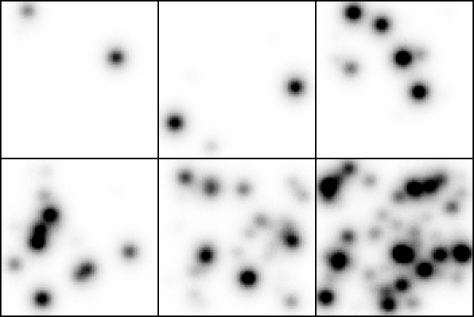
The influence of crowding is tested on six images with the same size, same PSF and same typical $S/N$ but different numbers of stars in the field, namely 3, 6, 12, 25, 50 and 100. All these images have $128\times 128$ pixels, the PSF has about 8 pixels FWHM and is constructed as the sum of two gaussians, a first one representing the core and a second one, about two times broader, accounting for the wings. These two gaussians have elliptical isopohotes but their major axes are perpendicular to each other, so that they cannot be well fitted by a Moffat function. This is not a very favourable case for our algorithm, since the analytical fit provides a rather poor approximation of the PSF and the numerical component is thus important.

The stars are positioned at random and their intensities are also randomly generated, with a uniform distribution in magnitude and a range of 7.5 mag (i.e. a factor 1000 in intensity). We add a sky background of about 30 e^-/pixel. The $S/N$ in the center of the stellar images varies from less than 1 for the faintest stars to about 70 for the brightest ones.

The six simulated images are displayed in Fig. 1, which shows that we go from isolated stars up to such a crowding that all stars are more or less severely blended: in the latter case, the average separation between stars is close to the PSF Full Width at Half Maximum (FWHM).

Figure 2: Difference between the reconstructed PSF and the exact one, as a function of crowding. The grey scale goes from $-2\%$ (white) to $+2\%$ (black) of the PSF peak intensity. From top left to bottom right: the PSF is determined from the fields containing 3, 6, 12, 25, 50 and 100 stars.

Figure 3: Standard deviation of the PSF residuals (in logarithmic scale) versus logarithm of the number of stars in the field. Long dashes: PSF constructed from the image of the brightest star in the field, assumed to be perfectly centered and isolated. Short dashes: PSF constructed from the images of all stars in the field, assumed to be perfectly centered and isolated. Continuous line: Our results.

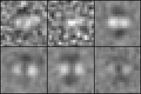
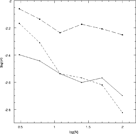
The differences between the reconstructed PSFs and the exact ones are shown in Fig. 2, for the six cases considered. The standard deviation of these residuals is computed in a circular aperture centered on the PSF and of 32 pixels diameter, i.e. 4 times the PSF FWHM. This is the area where the PSF intensities may be considered significant ($>1\%$ of the peak intensity). These standard deviations, in units of the PSF peak intensity, are plotted in Fig. 3 and compared with the results which would be obtained in two special cases. First, the PSF which would be given by the image of the brightest star in the field, should it be completely isolated and, secondly, the PSF which would be deduced from all stars in the field, should they all be isolated. Fig. 3 shows, first, that the recovered PSF is always more accurate than what would be deduced from the image of the brightest star, the improvement increasing with the crowding of the field. This means that the advantage provided by the additional signal more than compensates the handicap due to blending. In the first four images (number of stars less than 50), our recovered PSF is even better than the one which would be obtained by summing all the stars in the field, if they were isolated. Although this might appear unphysical, this is due to the way we determine the PSF, first by the fit of an analytical function, then by imposing a smoothing constraint on the numerical residuals. This results in a rather efficient correction for the photon noise, which has Fourier components at significantly higher frequencies than our well sampled PSF. When the number of stars grows, the relative photon noise decreases and its reduction by the algorithm cannot compensate anymore for the effect of blending, which also becomes more and more severe.

The accuracy of the photometry is checked in the following way. First, we compute the error $\delta a_{i}$ in the intensity of the source $a_{i}$, which is also the total flux in the stellar image since the PSF is normalized. This error is simply the value returned by the algorithm minus the exact value used to build the simulated image. Then, we compute a theoretical estimate of the standard error by assuming that the PSF is fitted by least squares on the image of a single (eventually blended) star, and that all other stars have previously been perfectly fitted (i.e. with their exact positions and intensities). This gives:

$$\frac{\sigma(a)}{a}=[\sum_{j}(\frac{as_{j}}{\sigma_{j}})^{2}]^{-1/2}$$ (8)

where the sum runs over all pixels.

Note that, in the case of a single star and no sky background, this formula reduces to $\frac{\sigma(a)}{a}=\sqrt{a}$, i.e. pure Poisson noise, as expected. The extra noise due to blends is taken into account in $\sigma_{j}$, in which the noise corresponding to all stars is included. Thus, all stars blending the star considered will contribute to an increase of the uncertainty. However, this formula does not take into account errors in the photometry due to inaccurate fitting of the neighbouring stars (i.e. it neglects the covariance terms) and is thus expected to be somewhat optimistic.

The accuracy of the photometry is quantified by:

$$\chi_{a}^{2}=\sum_{i}(\frac{\delta a_{i}}{\sigma(a_{i})})^{2}$$ (9)

where the sum is over all stars in the field. The reduced $\chi_{a}^{2}$ ($\chi_{a}^{2}$ divided by the number of stars) is expected to be close to 1 if everything works fine. Indeed, it fluctuates between 0.68 and 1.62, with an average value of 1.03, which means (1) that our photometric errors are perfectly compatible with the noise in the image and (2) that the correlated errors do not contribute much to the global $\chi_{a}^{2}$. Moreover, no significant trend with crowding appears, meaning that the strongest crowding considered (average separation $\sim$ FWHM of the PSF) is not severe enough to jeopardize our photometric results.

Figure 4: Difference between the reconstructed PSF and the exact one, as a function of $S/N$. The grey scale goes from $-2\%$ (white) to $+2\%$ (black) of the PSF peak intensity. From top left to bottom right: the PSF is determined from fields with increasing $S/N$ (see text).

4.2 Influence of $S/N$

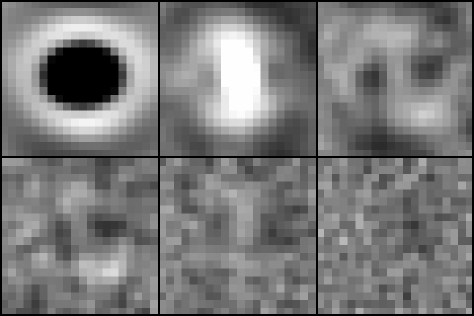
The influence of $S/N$ on the PSF accuracy is tested in a similar way. We use the image with 50 stars discussed in the previous subsection and vary the exposure level over a large range, i.e. from 30 to 10000 e^-/pixel in the center of the brightest star. This corresponds to an integrated $S/N$ varying from about 20 to 1000 for the brightest star in the field.

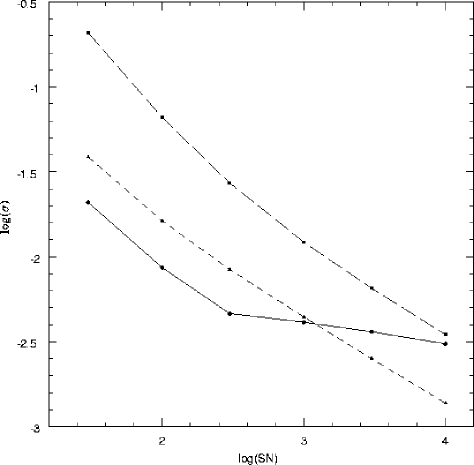
The differences between the reconstructed PSFs and the exact ones are shown in Fig. 4. The standard deviation of these residuals is computed in the same circular aperture as above and compared with the same 2 cases as in the previous subsection. Figure 4 shows that our results are always better than the ones which would be obtained from the brightest star, in case it would be isolated. At low to moderate $S/N$ (brightest star peak intensity $<1000$ e^-, integrated $S/N<300$), our results are also better than what would be obtained from summing all stellar images, assuming they were isolated. Again, this is due to the fact that the smoothing term reduces the effect of the photon noise. At high $S/N$ (400 to 1000), the contribution of the photon noise becomes relatively smaller and its reduction does not compensate anymore for the degradation due to crowding. Nevertheless, the accuracy of the recovered PSF continuously improves with increasing $S/N$, as expected.

The accuracy of the photometry as a function of $S/N$ is quantified in the same way as in the previous subsection. As the $S/N$ increases, the photometry gets more and more accurate, but not quite as much as Eq. (8) predicts. Indeed, this equation does not take into account errors coming from inaccuracies in neighbouring stars (correlated errors). At low $S/N$, these correlated errors are much lower than the random ones. However, as the random errors obviously decrease with increasing $S/N$, the correlated errors start to play a role, and the reduced $\chi_{a}^{2}$ grows from $\sim 1$ at low $S/N$ to 1.5 at $S/N\sim 500$ and 1.9 at $S/N\sim 1000$ (the indicated $S/N$ are integrated ones for the brightest star in the field). Thus, even at the highest $S/N$, the photometric errors are only about $40\%$ larger than would be expected in the ideal case (zero correlation). We should also note that they can be reduced if the stars’positions can be constrained from many observations, as is the case in a photometric monitoring.

Figure 5: Standard deviation of the PSF residuals (in logarithmic scale) versus logarithm of peak intensity (see text). Long dashes: PSF constructed from the image of the brightest star in the field, assumed to be perfectly centered and isolated. Short dashes: PSF constructed from the images of all stars in the field, assumed to be perfectly centered and isolated. Continuous line: Our results.

Figure 6: Top left: H-band (F160W) HST/NICMOS observation of the gravitational lens WFI2033$-$4723. Top right: simultaneous deconvolution of 4 such images, on a $2\times 2$ smaller pixel grid with 3 (small) pixels FWHM, shown on the same intensity scale. Bottom left: PSF kernel $\@vec{s(x)}$ determined from a deconvolution of the Tiny Tim PSF. A logarithmic intensity scale is used to enhance the faint structures. Bottom right: numerical component added to PSF, as determined by the present method. In this panel, the zero level is grey, lighter areas correspond to negative differences and darker ones to positive ones, the grey scale goes from $-10\%$ to $+10\%$ of the PSF peak intensity.

5 PSF determination and simultaneous deconvolution of several images

One of the main applications of the MCS algorithm, in its original form, was to deconvolve not only an image of a given object, but also a whole set of images of the same object. In such a case the deconvolution process computes a unique sharpened image compatible with all the images of the dataset simultaneously, hence the name simultaneous deconvolution. This specificity of the MCS algorithm has been transposed to the present method. It allows to determine simultaneously the PSFs for a series of images. If the individual images have been taken at different epochs, the intensities of all point sources in the field are left free during the deconvolution process, leading to the construction of a genuine light curve for all objects.

In such a case, instead of seeking the minimum of a function ${\cal S}$ which is the sum of a $\chi^{2}$ and a smoothing term (Eq. 5), one seeks the minimum of a function which is the sum of a $\chi^{2}$ for each of the images considered plus one smoothing term per image. The PSFs and the source intensities are allowed to vary from image to image, but the source positions are common to all images. A translation of the whole image is however allowed, to account for different centerings of the various exposures. All these parameters (source positions, source intensities, translations and PSF shapes) are simultaneously determined by the minimization algorithm.

5.1 HST/NICMOS observations of a gravitational lens

Even if the method presented here assumes that the data only contain point sources, one can adapt the algorithm to allow it to take into account faint diffuse objects.

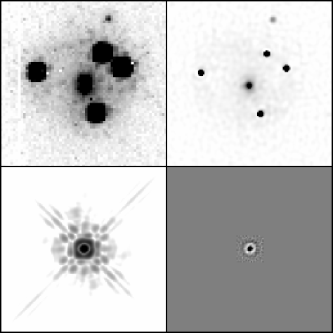
WFI2033$-$4723, a quadruply imaged quasar lensed by a distant galaxy, provides a typical case where such a strategy can be applied. The top left panel of Fig. 6 shows a $H-$band HST/NICMOS observation of that gravitational lens.

A deconvolution of the Tiny Tim PSF (Krist and Hook TinyTim (2004)) is used as a first approximation of $s(\@vec{x})$, which is then modified to provide the best possible deconvolution of the input image, which is first assumed to contain only four point sources. As the image actually contains a diffuse background (the lensing galaxy) in addition to the point sources, part of that background is interpreted as increased PSF wings and another part appears in the residuals (observed image minus reconvolved model). This latter part may be subtracted from the original image, which thus allows to correct for a part of the diffuse background. That corrected image may then be used to obtain an improved PSF.

Applying that procedure iteratively allows to obtain a PSF which, at each iteration, contains a smaller contamination by the diffuse background. Once that procedure has converged, the PSF is used as input for deconvolution of the original image by the classical MCS algorithm, including a diffuse background.

The result is shown in the top righ panel of Fig. 6. The bottom left panel of Fig. 6 shows the PSF kernel $s(\@vec{x})$ obtained from deconvolving the PSF computed with the Tiny Tim software while the bottom right panel shows the numercial component which has to be added to the former PSF kernel in order to obtain a good deconvolution of the input image.

This method has been applied to more complex cases, as the Cloverleaf gravitational lens H1413+117 (Magain et al. Magain88 (1988)). In that case, it allows to detect the lensing galaxy as well as part of an Einstein ring, which is completely hidded in the original data (Chantry, Magain & Courbin, in preparation).

5.2 Example: detailed light curve of a faint Mira in the halo of NGC5128, Cen A

With the increasing performances of modern telescopes, it becomes possible to study the stellar populations of objects that were so far unresolved under standard seeing conditions, around 1″. One can even start to resolve (nearby) galaxies into stars and to construct actual colour-magnitude diagrams. However, while the resolution of the observations improves, the field of view often decreases, making it very difficult or even impossible to observe at the same time the field of interest and the relatively bright, isolated stars generally required to build the PSF.

The search for faint blended variable stars in nearby galaxies is one of the topics directly influenced by the quality of the available PSF. Rejkuba et al. (Marina (2003)) have found dozens of Mira stars in the halo of the giant elliptical galaxy NGC 5128 (Centaurus A), but also note that strong blends often hamper the accurate measurement of periods. This occurs because the Mira itself can be in a close blend, but also often because the field where it lies is far away from any suitable PSF star. Our method computes the PSF directly from all the stars, blended or not, in the field of view, hence taking advantage of the total $S/N$ of all available point sources. The PSF is also well representative of the instrumental/atmospheric blurring at the position of the object of interest in the image.

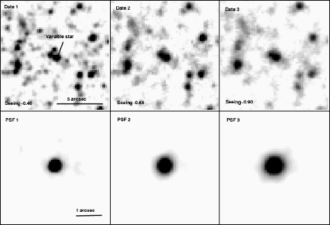
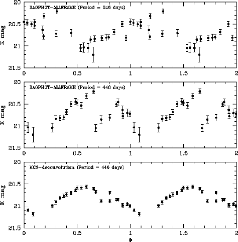
We have selected one of the Mira candidates found by Rejkuba et al. (Marina (2003)) using VLT K-band images. The region used for the deconvolution is a subset of the whole image obtained. Fig. 7 presents a sample of three images of the same field, taken at different epochs, with very different seeings. The photometry of the Mira star has been carried out on the 21 data frames available and a phase diagram could be constructed, as displayed in the bottom panel of Fig. 8. The photometric uncertainties, estimated from the scatter in the light curve of a constant star of the same magnitude as the Mira, amount to 0.05 mag, as compared to an average of 0.15 mag with the PSF-fitting method. Not only the error bars on the individual photometric points improve by a factor of almost 3 when compared with classical methods (top and middle panels of Fig. 8), but also the period obtained is different. The frequency peaks found in the Fourier analysis of the light curves with the present algorithm are much stronger than with the classical method. The 446 day period is clearly pointed out by the Fourier analysis, while the 246 day period supported by the classical PSF fitting no more yields a prominent peak.

Figure 7: Zoom on a Mira star in the halo of the radio galaxy NGC 5128 (Centaurus A), selected from Rejkuba et al. Marina (2003). Three VLT K-band images with very different seeing conditions are shown on the top panels. The exposure time is the same in all three exposures: 3600sec. The pixel size is 0.144″. The three PSFs in the bottom panels were obtained using the simultaneous deconvolution algorithm presented here. The pixel size is now 0.072″. These PSFs are the PSF kernels to be used in the MCS algorithm to improve the data from their original resolution, to a better and common resolution of 3 pixels FWHM, i.e., 0.22″.

Figure 8: Top panel: Light curve (shown here as phase diagram) of the Mira presented in Fig. 7, as obtained with standard PSF fitting techniques (DAOPHOT-ALLFRAME). The PSFs are computed independently in the individual frames from relatively isolated stars in the field of view, well outside the field of Fig. 7. The 1$\sigma$ error bar on the photometric points is $\sim 0.15$ mag. The period found from Fourier techniques is 246 days. Middle panel: Phase diagram constructed from the same data points, but with the 446 days period determined from our improved photometry. Bottom panel: Phase diagram obtained from the same images and the algorithm presented here. The 1$\sigma$ error bar is now 0.05 magnitude and the scatter between the points is drastically improved. The new period measured is 446 days, completely different from the period measured with standard photometric techniques.

6 Conclusion

The deconvolution-based algorithm presented here has been designed to compute accurate PSFs in fields very crowded with point sources. It not only computes the PSF but also provides the photometry and astrometry of all point sources in the field of view. The algorithm can be applied to single images or to a set of images of a given field. In the latter case, the images are processed simultaneously, in the sense of the MCS deconvolution algorithm: a PSF is computed for each image, by considering all images simultaneously. The photometry of all points sources is obtained for all images in the dataset, i.e., light curves are directly produced.

The method is clearly useful when few or no isolated PSF stars are available in the field of view, in the case of extreme crowding and in the case of strong PSF variation accross the field (in which case the PSF has to be determined from stars very close to the target). It is also very efficient in extracting photometric information from datasets of very heterogeneous quality (e.g., with a broad range of seeing values). In this case, the astrometry of the points sources in the best seeing data effectively constrains the astrometry of the bad seeing data, as long as all the data are processed simultaneously.

Although the present method is not designed to handle images that consist in a mixture of point sources and extended ones, it can cope with extended objects which are faint in comparison to the point sources, by running the algorithm in an iterative way.