The Evolving Luminosity Function of Red Galaxies

Michael J. I. Brown^1†^1†affiliationmark: , Arjun Dey²²affiliation: National Optical Astronomy Observatory, Tucson, AZ 85726-6732, USA , Buell T. Jannuzi²²affiliation: National Optical Astronomy Observatory, Tucson, AZ 85726-6732, USA , Kate Brand²²affiliation: National Optical Astronomy Observatory, Tucson, AZ 85726-6732, USA , Andrew J. Benson³³affiliation: Department of Physics, University of Oxford, Keble Road, Oxford OX1 3RH, UK ⁴⁴affiliation: California Institute of Technology, 1200 E. California Blvd., Pasadena, CA 91125, USA , Mark Brodwin⁵⁵affiliation: Jet Propulsion Laboratory, California Institute of Technology, 4800 Oak Grove Drive, Pasadena, CA 91109, USA Darren J. Croton⁶⁶affiliation: Department of Astronomy, University of California at Berkeley, Mail Code 3411, Berkeley, CA 94720, USA , Peter R. Eisenhardt⁵⁵affiliation: Jet Propulsion Laboratory, California Institute of Technology, 4800 Oak Grove Drive, Pasadena, CA 91109, USA mbrown@astro.princeton.edu

Abstract

We trace the assembly history of red galaxies since $z=1$ , by measuring their evolving space density with the $B$ -band luminosity function. Our sample of 39599 red galaxies, selected from $6.96~{}{\rm deg}^{2}$ of imaging from the NOAO Deep Wide-Field and Spitzer IRAC Shallow surveys, is an order of magnitude larger, in size and volume, than comparable samples in the literature. We measure a higher space density of $z\sim 0.9$ red galaxies than some of the recent literature, in part because we account for the faint yet significant galaxy flux which falls outside of our photometric aperture. The $B$ -band luminosity density of red galaxies, which effectively measures the evolution of $\sim L^{*}$ galaxies, increases by only $36\pm 13\%$ from $z=0$ to $z=1$ . If red galaxy stellar populations have faded by $\simeq 1.24$ $B$ -band magnitudes since $z=1$ , the stellar mass contained within the red galaxy population has roughly doubled over the past $8~{}{\rm Gyr}$ . This is consistent with star-forming galaxies being transformed into $\lesssim L^{*}$ red galaxies after a decline in their star formation rates. In contrast, the evolution of $\simeq 4L^{*}$ red galaxies differs only slightly from a model with negligible $z<1$ star formation and no galaxy mergers. If this model approximates the luminosity evolution of red galaxy stellar populations, then $\simeq 80\%$ of the stellar mass contained within today’s $4L^{*}$ red galaxies was already in place at $z=0.7$ . While red galaxy mergers have been observed, such mergers do not produce rapid growth of $4L^{*}$ red galaxy stellar masses between $z=1$ and the present day.

galaxies: evolution – galaxies: luminosity function, mass function – galaxies: elliptical and lenticular, cD

^†^†slugcomment: Preprint submitted to the ApJ¹¹affiliationtext: Princeton University Observatory, Peyton Hall, Princeton, NJ 08544-1001, USA^$\dagger$^$\dagger$affiliationtext: H.N. Russell Fellow

1 INTRODUCTION

Red galaxies contain the majority of the stellar mass at low redshift (Hogg et al. 2002), so understanding their formation and assembly is one of the key goals of both observational and theoretical extragalactic astronomy. The stellar populations of these galaxies are dominated by an old component, with little ongoing star formation (e.g., Tinsley 1968). Observationally, it is unclear if this star formation occurred in situ at $z>1$ , or if these stars formed in lower mass galaxies which were later assembled via galaxy mergers. Simulations of red galaxy evolution predict varying assembly and star formation histories, with some papers concluding that assembly takes place primarily at high redshift (e.g., Meza et al. 2003; Naab et al. 2005) while others suggest it continues today (e.g., De Lucia et al. 2006).

The color-magnitude diagram of low redshift galaxies provides several important clues about the assembly of red galaxies. At low redshift there is a tight locus of red galaxies in color-magnitude space (e.g., Bower, Lucey, & Ellis 1992; Hogg et al. 2004; McIntosh et al. 2005), with the most luminous red galaxies being slightly redder than less luminous red galaxies. This indicates that red galaxies of a given luminosity and metallicity have similar star formation histories, at least over the last few ${\rm Gyr}$ . A red galaxy locus is also observed within the $z\sim 1$ cluster and field galaxy populations (van Dokkum et al. 2000; Blakeslee et al. 2003; Bell et al. 2004; Willmer et al. 2005). The absence of very massive star-forming galaxies at low redshifts indicates that the most massive red galaxies are either formed at high redshift or they are assembled via mergers at $z<1$ . As the colors of red galaxies are a function of luminosity, mergers of red galaxies should produce galaxies slightly blueward of the color-magnitude relation, and thus increase the scatter within the relation.

Mergers of red galaxies, perhaps without significant merger-triggered star formation (dry mergers), have been observed at low redshift (e.g., Lauer 1988; van Dokkum 2005), but it is unclear how large a role they play in galaxy formation. While there have been valiant attempts to measure the galaxy merger rate with redshift (e.g., Le Fèvre et al. 2000; Bell et al. 2006), there is debate about the selection function of merger candidates and the duration of observable galaxy mergers. At low redshift, measured rates of red galaxy stellar mass growth via mergers span from $\simeq 1\%$ per ${\rm Gyr}$ (Masjedi et al. 2006) to $\simeq 10\%$ per ${\rm Gyr}$ (van Dokkum 2005).

The space density of red galaxies with redshift is a relatively direct measure of the galaxy assembly history, and has fewer uncertainties than measurements of the galaxy merger rate. At the redshifts where galaxy assembly takes place, the space density of galaxies as a function of stellar mass will evolve with redshift. While conceptually simple, it is difficult to measure the galaxy space density accurately, as $z=1$ $L^{*}$ red galaxies are optically faint and their strong spatial clustering (e.g., Brown et al. 2003) results in significant cosmic variance. Despite these difficulties, several groups have used measurements of the space density of galaxies with redshift to constrain red galaxy evolution and assembly (e.g., Lilly et al. 1995; Lin et al. 1999; Chen et al. 2003; Bell et al. 2004; Bundy et al. 2005; Willmer et al. 2005; Wake et al. 2006). Faber et al. (2005) provides a useful summary of prior studies, and describes their varying conclusions. The prior literature provides several plausible scenarios for $z<1$ red galaxy evolution, including passive evolution, assembly via dry mergers, formation from fading blue galaxies, or a combination of the above.

This is the first in a series of papers which will discuss the assembly and evolution of $z<1$ red galaxies detected by the multiwavelength imaging surveys of the entire Boötes field. Other papers in this series will measure the stellar mass function, spatial clustering, and AGN content of red galaxies. In this paper we present the evolving $B$ -band luminosity function of $0.2<z<1.0$ red galaxies, and discuss the resulting implications for red galaxy evolution and assembly. While the rest-frame $B$ -band is not ideal for tracing stellar mass, it has the advantages of being within the well studied optical wavelength range and remaining within the observed $B_{W}RI$ passbands of the NOAO Deep Wide-Field Survey (NDWFS) for redshifts of $z<1$ .

The structure of this paper is as follows. We provide an overview of the NDWFS and Spitzer IRAC Shallow Survey in §2. We discuss our catalogs, photometry, photometric redshifts, and galaxy rest-frame properties in §3. In §4 we describe the selection of our red galaxy sample. In §5 we present rest-frame $B$ -band luminosity functions of red galaxies and compare our measurements with simple galaxy evolution models. In §6 we compare our results with recent red galaxy surveys, and discuss discrepancies between various studies. Our principal results and conclusions are summarized in §7. Throughout this paper we use Vega based magnitudes and adopt a cosmology of $\Omega_{m}=0.3$ , $\Omega_{\Lambda}=0.7$ , $H_{0}=70~{}{\rm km}~{}{\rm s}^{-1}~{}{\rm Mpc}^{-1}$ , $h=0.7$ , and $\sigma_{8}=0.8$ .

2 THE SURVEYS

2.1 The NOAO Deep Wide-Field Survey

The NOAO Deep Wide-Field Survey (NDWFS) is an optical ( $B_{W}RI$ ) and near-infrared ( $K$ ) imaging survey of two $\approx 9.3~{}{\rm deg}^{2}$ fields with telescopes of the National Optical Astronomy Observatory (Jannuzi & Dey 1999). A thorough description of the observing strategy and data reduction will be provided by B. T. Jannuzi et al. and A. Dey et al. (both in preparation). We utilize the third NDWFS data release¹¹1Available from the NOAO Science Archive at http://www.archive.noao.edu/ndwfs/ of optical imaging with the MOSAIC-I camera on the Kitt Peak 4-m telescope. To obtain accurate optical colors with fixed aperture photometry across the Boötes field, we have smoothed copies of the released images so the stellar Point Spread Function (PSF) is a Moffat profile with a full width at half maximum of $1.35^{\prime\prime}$ and $\beta=2.5$ . The subfield ${\rm NDWFSJ1428+3531}$ (each subfield is roughly one MOSAIC-I field-of-view) has poor seeing in the $B_{W}$ and $R$ -bands, and has been excluded from this study.

2.2 The IRAC Shallow Survey

The IRAC instrument (Fazio et al. 2004) on the Spitzer Space Telescope provides simultaneous broad-band images at $3.6$ , $4.5$ , $5.8$ , and $8.0~{}\mu{\rm m}$ . The IRAC Shallow Survey, a guaranteed-time observation program of the IRAC instrument team, covers $8.5~{}{\rm deg^{2}}$ of Boötes with three or more 30 second exposures per position. Eisenhardt et al. (2004) present an overview of the survey design, reduction, calibration, and preliminary results. Despite the short integration times, the IRAC Shallow Survey easily detects $z\sim 1.4$ cluster galaxies (Stanford et al. 2005; Elston et al. 2006; Brodwin et al. 2006). In this paper we utilize the $3.6$ and $4.5~{}\mu{\rm m}$ imaging to remove contaminants (e.g., stars, quasars) from our galaxy sample and for empirical photometric redshifts. The observed $I-[3.6]$ color of $z<1$ red galaxies is a superb redshift indicator, due to the redshifting of the $1.6~{}\mu{\rm m}$ ${\rm H}^{-}$ stellar opacity feature (e.g., Simpson & Eisenhardt 1999; Sawicki 2002).

3 THE OBJECT CATALOG

3.1 OBJECT DETECTION

We detected sources using SExtractor $2.3.2$ (Bertin & Arnouts 1996), run in single-image mode on the $I$ -band images of the NDWFS third data release. The NDWFS Boötes field comprises of 27 optical subfields, each of which are $35^{\prime}\times 35^{\prime}$ in size, that are are designed to have overlaps of several arcminutes. Individual objects can be detected in multiple subfields, which is particularly useful for photometric calibration, though the effective exposure time generally decreases towards subfield edges. For this paper, we only include objects which are detected within nominal subfield boundaries, which we define to have overlaps of only tens of arcseconds. In these small overlap regions, we search for objects with $I$ -band detections in multiple subfields and retain the detection with the highest quality data (i.e., without bad pixels or with the longest exposure time). To minimize the number of faint spurious galaxies in our catalog, we exclude regions surrounding very extended galaxies and saturated stars. We also exclude regions that do not have good coverage from both the NDWFS and the IRAC Shallow Survey. The final sample area is $6.96~{}{\rm deg}^{2}$ over a $2.7^{\circ}\times 3.3^{\circ}$ field-of-view.

3.2 PHOTOMETRY

We used our own code to measure aperture photometry for each object in the optical and IRAC passbands. To reduce contaminating flux from neighboring objects, we used SExtractor segmentation maps to exclude pixels associated with neighboring objects detected in any of the three optical bands. We corrected the aperture photometry for missing pixels (from the segmentation maps or bad pixels) by using the mean flux per pixel measured in a series on $0.5^{\prime\prime}$ wide annuli surrounding each object position. Accurate $1\sigma$ uncertainties for the photometry were determined by measuring photometry at $\simeq 100$ positions within $2^{\prime}$ of the object position and finding the uncertainty which encompassed 68.7% of the measurements. We also use the median of the fluxes measured at these positions to subtract small errors which could be present in our sky background estimate. Typical random uncertainties for $I$ -band $4^{\prime\prime}$ diameter aperture photometry are $0.03$ magnitudes at $I=21$ , increasing to $0.2$ magnitudes at $I=23$ . Typical random uncertainties for $3.6~{}\mu{\rm m}$ $4^{\prime\prime}$ aperture photometry are $0.02$ magnitudes at $[3.6]=16$ , increasing to $0.2$ magnitudes at $[3.6]=19$ .

Refer to caption — Figure 1: The offset between measured and total photometry for $4^{\prime\prime}$ aperture photometry (left) and SExtractor’s MAG_AUTO (right). We only plot galaxies over the apparent magnitude range where the completeness is 50% or more, and we treat non-detections as measurements of $I=99$ . The predicted offsets due to flux outside the $4^{\prime\prime}$ aperture are shown with arrows, and these are consistent with our measurements. SExtractor’s MAG_AUTO photometry is closer to total magnitudes than $4^{\prime\prime}$ aperture photometry, but has systematics as a function of both half-light radius and apparent magnitude. Luminosity functions using MAG_AUTO for total magnitudes may have systematics as a function of both luminosity and redshift.

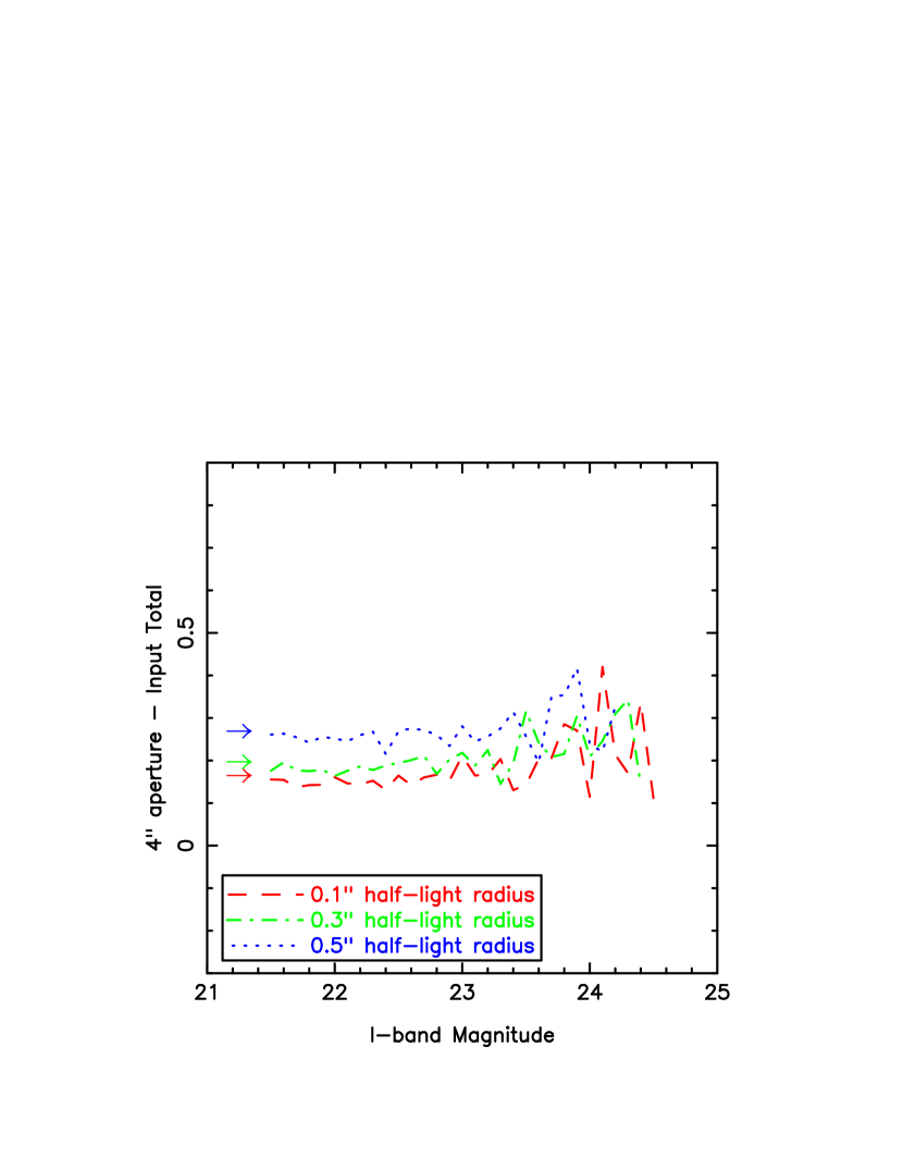
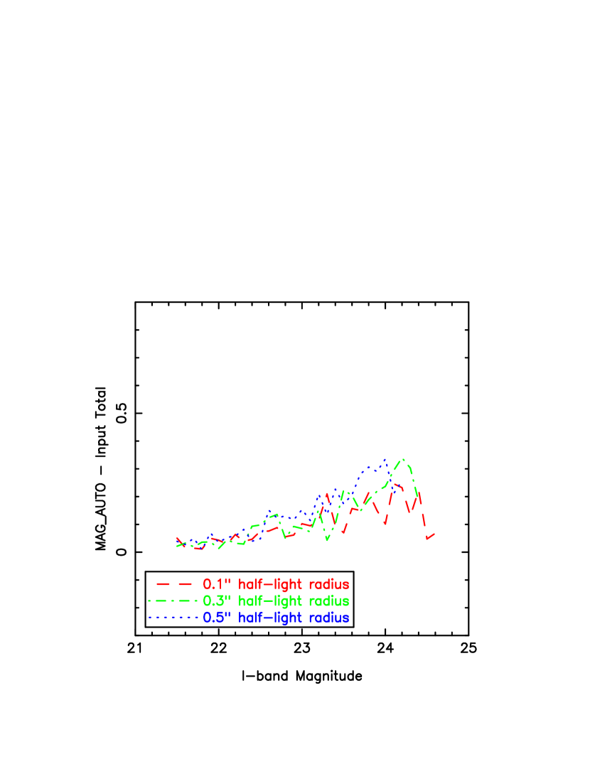
To verify the accuracy of our uncertainties and to search for systematic errors, we added artificial galaxies to our data, recovered them with SExtractor, and measured their photometry. The artificial galaxies have de Vaucouleurs (1948) profiles truncated at seven half-light radii (though our results are not particularly sensitive to the truncation radius), which were then convolved with our PSF. Figure 1 plots the offset between total and measured luminosities for these galaxies. This offset is due to flux outside outside of our $4^{\prime\prime}$ diameter aperture, and is a predictable function of half-light radius. The observed half-light radius is a function of both galaxy luminosity and redshift, and we discuss corrections from $4^{\prime\prime}$ aperture photometry to total magnitudes in §3.4. After accounting for this predicted offset, we find that the difference between the input and measured photometry is within the quoted $1\sigma$ uncertainties $\simeq 70\%$ of the time.

It is useful to compare our photometry with SExtractor’s ${\rm MAG\_AUTO}$ , which is often used to measure “total” magnitudes in galaxy surveys (e.g., Bell et al. 2004; Zucca et al. 2005). While SExtractor is an extremely useful tool for source detection, photometry and classification, it cannot be expected to provide perfect measurements of all objects in all surveys. Using the same artificial galaxies as described above, we find 80% of the MAG_AUTO measurements differ from the total magnitude by more than the quoted $1\sigma$ uncertainty. This is due to SExtractor’s assumption that the sky background is Gaussian random noise without source confusion, which is only a valid approximation for some imaging data.

We show in Figure 1 that MAG_AUTO is closer to a total magnitude than $4^{\prime\prime}$ aperture photometry, though it has systematic errors which are a function of apparent magnitude. In addition, its random errors are 40% larger than $4^{\prime\prime}$ aperture photometry. The systematic error with magnitude may be due to the elliptical MAG_AUTO aperture being defined using the second-order image moments of object pixels above an isophotal threshold. It is therefore plausible that the MAG_AUTO aperture is slightly too small for relatively extended faint galaxies. Luminosity functions using MAG_AUTO for total magnitudes may have systematics of $\sim 0.2$ magnitudes at faint magnitudes, though the exact size of this offset will depend both on the imaging data and user defined SExtractor parameters. Accurate luminosity functions require corrections for galaxy flux which falls beyond the photometric aperture.

3.3 PHOTOMETRIC REDSHIFTS

We determined redshifts for our galaxies using the empirical ANNz photometric redshift code (Firth, Lahav, & Somerville 2003; Collister & Lahav 2004). When a sufficiently large training set is available, empirical photometric redshifts are as precise or better than other techniques (e.g., Csabai et al. 2003; Brodwin et al. 2006). This approach does restrict us to $z<1$ , where thousands of spectroscopic redshifts are available in Boötes to calibrate the photometric redshifts. ANNz uses artificial neural networks to determine the relationship between measured galaxy properties and redshift. It does not use any prior assumptions about the shape of galaxy spectral energy distributions (SEDs), though it does assume the relationship between galaxy properties and redshift is a relatively smooth function. ANNz works best when the training set is a large representative subset of the science galaxy sample.

The basis of our training set is galaxies with spectroscopic redshifts in the Boötes field. The ongoing AGN and Galaxy Evolution Survey (AGES, C. S. Kochanek et al. in preparation) of Boötes has obtained spectroscopic redshifts of $\simeq 16000$ $I\lesssim 20$ galaxies, using the MMT’s Hectospec multiobject spectrograph (Fabricant et al. 2005). At fainter magnitudes, most of the spectroscopic redshifts are from various spectroscopic campaigns with the W. M. Keck, Gemini, and Kitt Peak observatories, which have jointly resulted in redshifts for several hundred galaxies.

We trained and measured photometric redshifts using the $4^{\prime\prime}$ aperture photometry and the 2nd order moments of the $I$ -band light distribution. For training and determining photometric redshifts we used ${\rm asinh}$ magnitudes (Lupton, Gunn, & Szalay 1999) rather than fluxes or conventional $2.5{\rm log}_{10}$ magnitudes. ANNz does not produce accurate photometric redshifts with fluxes that span a vast dynamic range, while conventional magnitudes only measure positive fluxes. We only use ${\rm asinh}$ magnitudes when estimating ANNz photometric redshifts and use conventional magnitudes throughout the remainder of the paper. The second order image moments are useful for reducing the number of bright galaxy photometric redshifts with large errors. In particular, they reduce photometric redshift outliers produced by low redshift edge-on spirals whose dust lanes produce colors similar to higher redshift objects. As we do not want the shape measurements to be a function of $I$ -band depth, which varies slightly across Boötes, we measure the 2nd order moments with pixels above an $I$ -band surface brightness of $22.5~{}{\rm mag}~{}{\rm arcsec}^{-2}$ .

We applied several restrictions to the training set to improve the photometric redshifts of $z<1$ red galaxies. We restricted the training set to $z<1.5$ spectroscopic galaxies, so $z>1.5$ galaxies did not perturb the ANNz photometric redshift solution for $z<1.5$ galaxies. While we include red galaxies with X-ray and radio counterparts in our final sample, these objects are overrepresented in our spectroscopic samples and a small fraction of these sources could have unusual colors due to the contribution of the AGN. We have therefore excluded objects with counterparts in the Chandra XBoötes survey (Kenter et al. 2005; Murray et al. 2005; Brand et al. 2006) or the FIRST radio survey (Becker, White, & Helfand 1995) from the photometric redshift training set. The small number of galaxies with unusual apparent colors which remained in the training set were removed with apparent color cuts which are a function of spectroscopic redshift.

At $z>0.6$ , there are only 280 red and blue galaxies fainter than $I=20.5$ with spectroscopic redshifts in the training set, which is less than ideal for training ANNz. As the shape of the galaxy color-locus at any given redshift is relatively simple and smooth, we were able to increase the size of the training set by adding interpolated objects to the training set. We did this when we found galaxies within 0.02 in redshift and within 0.5 in $B_{W}-R$ color of each other. As red galaxies at $z<1$ follow relatively tight color-magnitude (e.g., Bower et al. 1992; Bell et al. 2004; McIntosh et al. 2005) and size-luminosity relations (e.g., Bender, Burstein, & Faber 1992; Shen et al. 2003), we were able to extrapolate the training set to fainter magnitudes by making faint copies of bright objects with slightly altered photometry and image size parameters. As the colors and sizes of galaxies are a very strong function of redshift, approximations of the color-magnitude and size-luminosity relations at a given redshift are sufficient for the photometric redshift training set. Figure 2 plots the color-color and color-magnitude diagrams of training set galaxies at $z=0.80$ , along with interpolated and extrapolated objects.

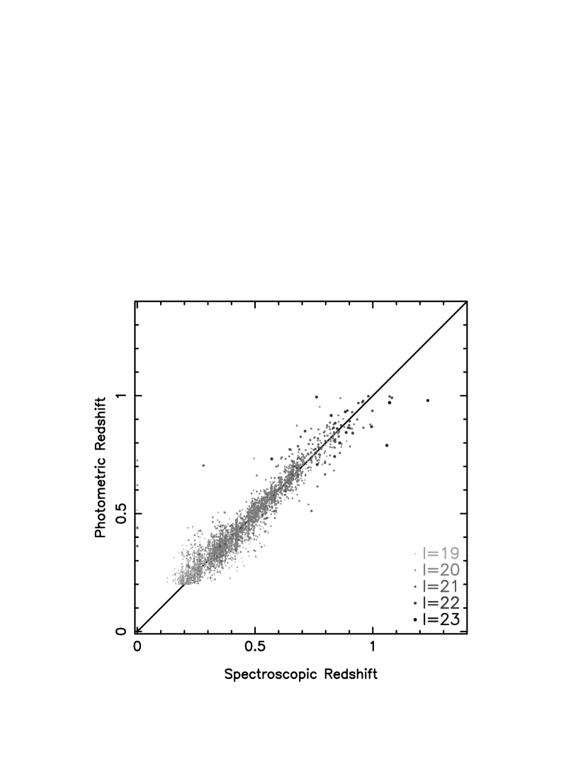
In Figure 3 we plot the photometric and spectroscopic redshifts of 4314 objects which meet our red galaxy selection criteria (which we discuss in §4), including radio and X-ray sources. We also provide estimates of photometric redshift uncertainties for a series of redshift and apparent magnitude bins in Table 1. The uncertainties were determined using the relevant percentiles, and do not assume a Gaussian distribution of photometric redshift errors. As the observed range of galaxy colors broadens with increasing apparent magnitude, at the very least due to photometric errors, the random errors of the photometric redshifts also increase with apparent magnitude. Measured systematic errors are much smaller than the random errors listed in Table 1. The accuracy of our red galaxy photometric redshifts are comparable to the best broad-band photometric redshifts available in the literature (e.g., Mobasher et al. 2004). The $1\sigma$ uncertainties of our photometric redshifts are $\simeq 0.1$ in redshift at $I=22$ , and this decreases to $\simeq 0.03$ at $I=19.5$ .

3.4 REST-FRAME PROPERTIES

To measure the rest-frame absolute magnitudes and colors of NDWFS galaxies, we used maximum likelihood fits of Bruzual & Charlot (2003) SED models to the $B_{W}RI$ $4^{\prime\prime}$ diameter aperture photometry. Throughout this paper we use solar metallicity models with a Salpeter (1955) initial mass function, a formation redshift of $z=4$ , and exponentially declining star formation rates. These models provide a reasonable approximation of the observed SEDs of red galaxies. Unlike empirical templates, the Bruzual & Charlot (2003) models allow us to estimate stellar masses and star formation rates, which we will use in future papers (K. Brand et al. and A. Dey et al., both in preparation). For this paper, we will only use the rest-frame optical colors and absolute magnitudes.

Other stellar population models can be fitted to red galaxies, though changing models has little impact on our $B$ -band luminosity functions and our conclusions. Shifting the formation redshift results in different $\tau$ models being fitted to the red galaxies, but the model $B$ -band luminosity evolution of red galaxy stellar populations at $z<1$ changes by $0.1$ magnitudes or less. Changing from a Salpeter (1955) to a Chabrier (2003) initial mass function decreases galaxy stellar masses by 25%, but has little impact on the predicted evolution of galaxy optical colors and luminosities. Models with low metallicities are bluer than the reddest galaxies, while models with 1.5 times Solar metallicity are offset from observed $B_{W}RI$ galaxy loci from $z=0.2$ to $z=1.0$ .

As with all current galaxy SED templates and models, there are small systematic errors. The $\tau$ models do not perfectly match the evolving rest-frame $U-V$ colors of red galaxies at all redshifts, and the $\tau$ models overestimate the apparent $R-I$ colors of $0.4\lesssim z\lesssim 0.7$ red galaxies by $\simeq 0.05$ magnitudes. As discussed in §6, we expect these systematics to have a modest impact on our luminosity functions.

The $4^{\prime\prime}$ aperture photometry captures 86% or less of the total flux. We corrected for the flux outside this aperture by assuming galaxies within our sample have truncated de Vaucouleurs (1948) profiles,

	$\displaystyle I$	$\displaystyle\propto$	$\displaystyle{\rm exp}\left[-7.6695\left(\frac{r}{r_{e}}\right)^{1/4}\right]$		(1)
			$\displaystyle-{\rm exp}\left[-7.6695\times 7^{1/4}\right]$		(1)

at $r<7r_{e}$ , where the half-light radius $r_{e}$ is a function of $B$ -band absolute magnitude and redshift. At $z=0$ , we use the size-luminosity relation of SDSS early-type galaxies (Shen et al. 2003) and assume $B_{\rm Vega}-r_{\rm AB}=1.32$ (Fukugita, Shimasaku, & Ichikawa 1995), so

{\rm log}[r_{e}({\rm h^{-1}kpc})]=1.0-0.26(M_{B}-5{\rm logh}+21.81).

(2)

The $1\sigma$ dispersion around this relation is only $30\%$ for the most luminous red galaxies (Shen et al. 2003), while the offsets between $4^{\prime\prime}$ and total magnitudes in Figure 1 are a relatively weak function of half-light radius. This simple relation should therefore provide accurate corrections between $4^{\prime\prime}$ aperture and total photometry.

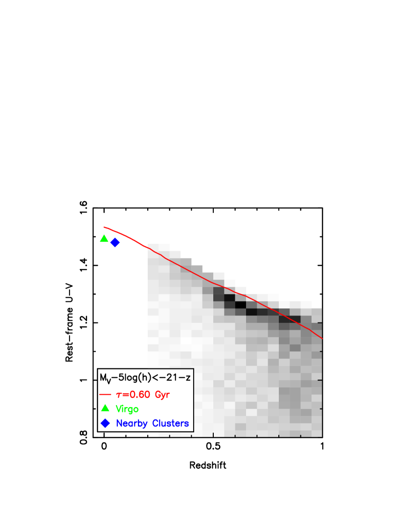
The size-luminosity relation must change with redshift due to the evolution of red galaxy stellar populations. We assume the size-luminosity relation undergoes pure luminosity evolution described by a Bruzual & Charlot (2003) $\tau=0.6~{}{\rm Gyr}$ stellar synthesis model with a formation redshift of $z=4$ . This model fades by $1.24$ $B$ -band magnitudes between $z=1$ and $z=0$ . As shown in Figure 4, the $\tau=0.6~{}{\rm Gyr}$ model approximates the color evolution of $M_{V}-5~{}{\rm log}~{}h\leq-21-z$ red galaxies. The luminosity evolution of the fundamental plane for $M_{B}-5~{}{\rm log}~{}h\simeq-20-1.2z$ early-type galaxies (e.g., van Dokkum & Stanford 2003; Treu et al. 2005) is also comparable to this model, though less luminous galaxies probably exhibit more rapid luminosity function (Treu et al. 2005; van der Wel et al. 2005). Stellar population synthesis models with $\tau<1~{}{\rm Gyr}$ have less than $2\%$ of their total star formation at $z<1$ . While this is a tiny amount of star formation, it does result in more rest-frame color and luminosity evolution than passive evolution models without any $z<1$ star formation. Changing the value of $\tau$ by $0.2~{}{\rm Gyr}$ alters the model $z=1$ rest-frame $U-V$ colors and $B$ -band luminosity evolution by $\simeq 0.1$ magnitudes. After accounting for the evolving size-luminosity relation and our $1.35^{\prime\prime}$ point spread function, we find the $4^{\prime\prime}$ diameter aperture captures 75% of the flux of a $M_{B}-5~{}{\rm log}~{}h=-21$ galaxy at $z=0.9$ .

Red galaxies do not exclusively have de Vaucouleurs (1948) profiles (e.g., Blanton et al. 2003; Driver et al. 2006), and this could affect our estimates of galaxy total magnitudes. To investigate this, we determined the offsets between $4^{\prime\prime}$ aperture and total magnitudes for Sersic (1968) profiles with indices between 2 and 6. For galaxies with half-light radii of $1^{\prime\prime}$ , the offset differs from that determined with a de Vaucouleurs (1948) profile by $0.03$ magnitudes. Changing the truncation radius from $7$ to $10$ half-light radii only changes the offset between $4^{\prime\prime}$ aperture and total magnitudes by $\sim 0.06$ magnitudes for galaxies with $r_{e}\sim 1^{\prime\prime}$ . This offset can be increased by using larger truncation radii, though this results in a systematic difference between the model and measured offset of $4^{\prime\prime}$ and $6^{\prime\prime}$ aperture photometry for red galaxies. As the expected evolution of red galaxy stellar populations is on the order of $1.24$ $B$ -band magnitudes per unit redshift, small errors in our corrections from $4^{\prime\prime}$ aperture to total magnitudes should have little impact upon our results and conclusions.

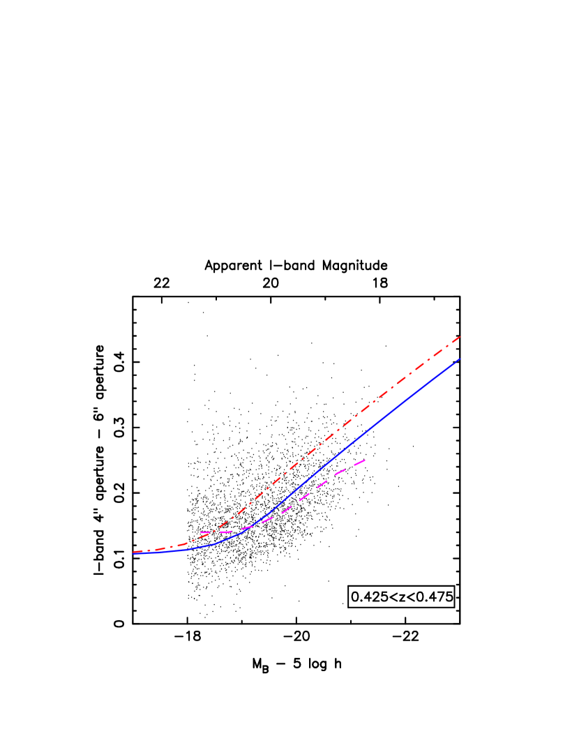
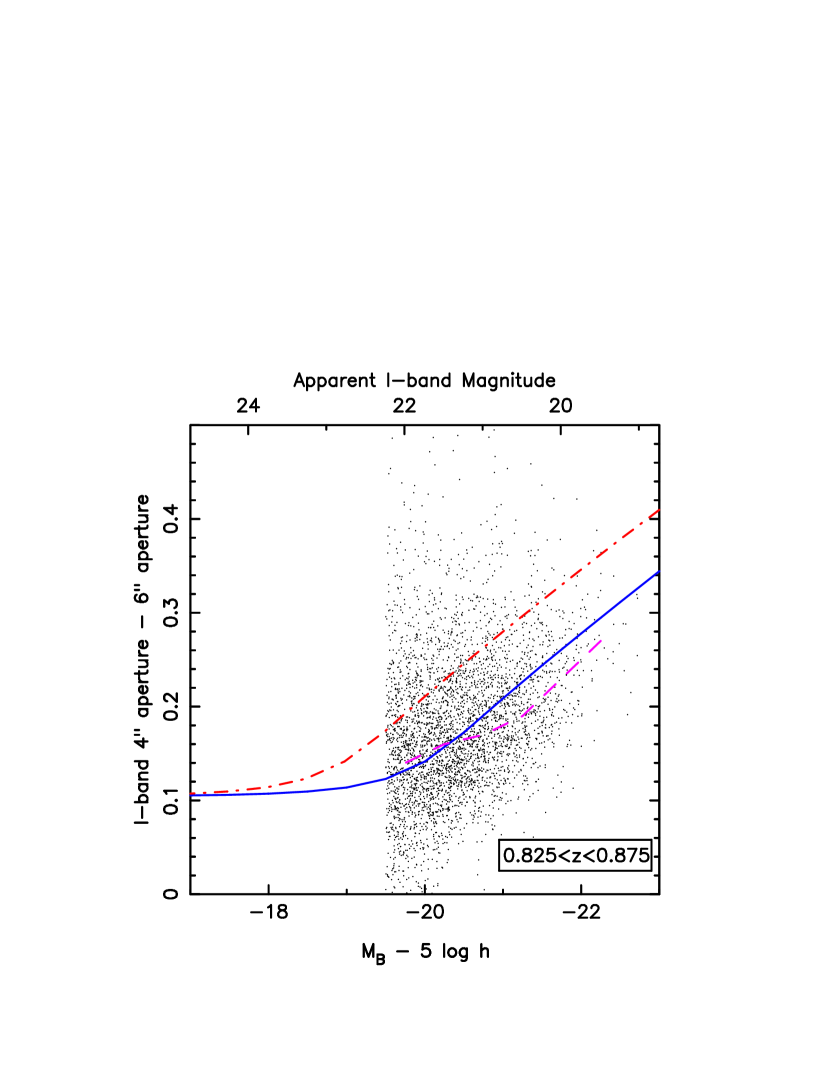
To verify the accuracy of our model, we compared the measured and predicted difference between $4^{\prime\prime}$ and $6^{\prime\prime}$ aperture photometry for red galaxies. As shown in Figure 5, our simple model provides a good approximation of what is observed in our red galaxy sample. Figure 5 also illustrates the absolute magnitude dependence of our model. This dependence results in the aperture corrections at fixed apparent $I$ -band magnitude increasing with redshift. It is therefore plausible that an estimator of total magnitudes could work well for the majority of $I=21$ galaxies, which are at $z<0.7$ , but have systematic errors for $I=21$ galaxies at $z=0.9$ . Accounting for flux outside the aperture is crucial for measuring the total magnitudes of $z<1$ galaxies.

4 THE RED GALAXY SAMPLE

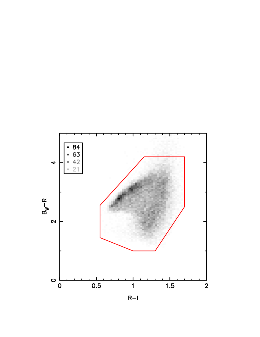
The rest-frame distribution of galaxy colors is bimodal (e.g., Hogg et al. 2004), and selection criteria for red galaxies typically fall near the minimum between the red and blue galaxy populations (e.g., Madgwick et al. 2002; Bell et al. 2004; Faber et al. 2005). We apply a similar approach for this work, and use the following rest-frame color selection criterion;

$\displaystyle U-V$	$\displaystyle>$	$\displaystyle 1.40-0.25$	(3)
		$\displaystyle-0.08\times(M_{V}-5~{}{\rm log}~{}h+20.0)$
		$\displaystyle-0.42\times(z-0.05)$
		$\displaystyle+0.07\times(z-0.05)^{2}.$

Our criterion selects galaxies with rest-frame $U-V$ colors within $0.25$ magnitudes of the evolving color-magnitude relation of red galaxies. This criterion allows comparison with the recent literature and is very similar, though not identical, to the criterion of Bell et al. (2004).

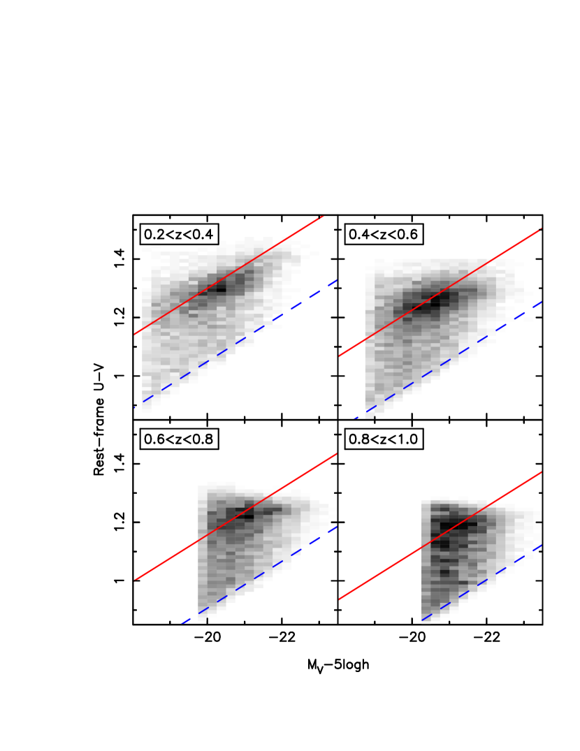
Our selection criterion is plotted in Figure 6 along with the observed color distribution of red galaxies. Our selection criterion has slightly more tilt than the observed color-magnitude relation of $0.2<z<0.4$ red galaxies. If we use $8^{\prime\prime}$ aperture photometry instead of $4^{\prime\prime}$ aperture photometry, the observed color-magnitude relation of $0.2<z<0.4$ red galaxies moves blueward and steepens. However, as this has little impact upon the measured luminosity function, we continue to use $4^{\prime\prime}$ aperture photometry, which has smaller random uncertainties than $8^{\prime\prime}$ aperture photometry.

The measured space density of the most luminous red galaxies does not depend on the details of our selection criterion, as these galaxies mostly lie along the color-magnitude relation. We can therefore easily compare our luminosity functions for $M_{B}-5~{}{\rm log}~{}h<-21$ red galaxies with those of 2dFGRS, SDSS, COMBO-17, and DEEP2 (Madgwick et al. 2002; Bell et al. 2004; Faber et al. 2005; Willmer et al. 2005; Blanton 2005), all of which use slightly different galaxy selection criteria. The fraction of blue galaxies increases with decreasing luminosity, so the measured space density of $\lesssim L^{*}$ red galaxies is a stronger function of the red galaxy selection criteria. If we shift our criterion blueward by $0.10$ magnitudes our measured space density of $M_{B}-5~{}{\rm log}~{}h\sim-20$ red galaxies increases by $\simeq 25\%$ .

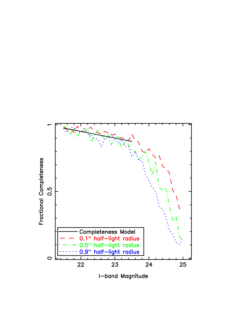
We limit the absolute magnitude range in each of our redshift bins so we can determine accurate redshifts and have a highly complete sample. Almost all of the galaxies in our final sample are detected in $B_{W}$ , $R$ , $I$ and the two IRAC bands. To evaluate the completeness of our sample, we added artificial galaxies to copies of the $I$ -band images and recovered them with SExtractor. The artificial galaxies had de Vaucouleurs (1948) profiles truncated at 7 effective radii, and we measure the completeness for a range of effective radii and apparent magnitudes. As illustrated in Figure 7, our catalogs are more than 85% complete for $I<23.5$ galaxies with half-light radii of $0.5^{\prime\prime}$ or less. Our measurements of the luminosity function, which we discuss in §5, include small corrections for this incompleteness.

4.1 ADDITIONAL SELECTION CRITERIA

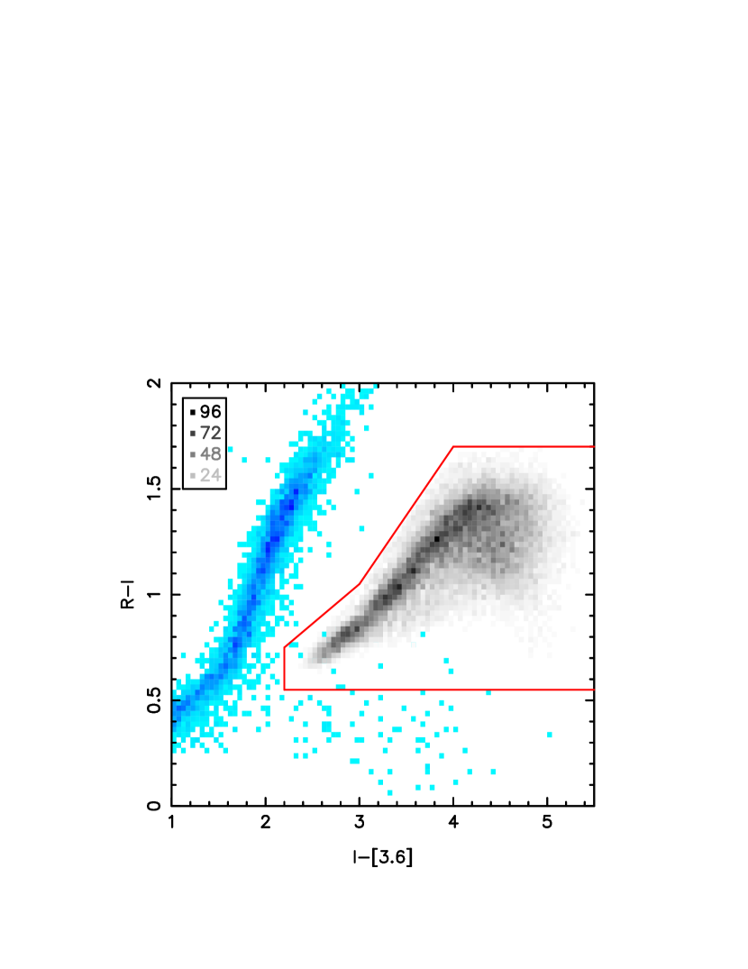
Contaminants cannot be rejected from photometric redshift surveys on the basis of their spectra, so these surveys can be more susceptible to contaminants than comparable spectroscopic surveys. This contamination can include stars, quasars, and galaxies with large photometric redshift errors. We therefore apply apparent color and morphology cuts to minimize contamination while retaining a highly complete sample of red galaxies.

We have applied apparent color cuts to exclude objects whose colors differ from those expected for $0.2<z<1.0$ red galaxies. These color cuts are designed to remove most stars, quasars and $z\gg 1$ galaxies from our sample. Our cuts may exclude a small percentage of red galaxies with unusually large photometric errors, but as these galaxies could also have large redshift and luminosity errors, it is preferable to exclude them from our measurement of the luminosity function. As the distribution of red galaxy apparent colors does not form a simple shape in color space, we use a total 17 color cuts to exclude objects from the sample. All but two of these cuts are plotted in Figure 8, while a full list is provided in Table 2.

Our color cuts remove 10767 objects from the sample, reducing it to 39866 objects. As we apply the color cuts before applying the morphology criterion, most of the objects rejected from the sample have the colors and morphologies of stars and quasars. Unlike $0.2<z<1.0$ red galaxies, main sequence stars have apparent colors which satisfy $R-I>0.65\times(I-[3.6]-1)$ or $I-[3.6]<2.2$ , and 8775 of the objects excluded by our color cuts satisfy these two criteria. Another 749 of the excluded objects satisfy $[3.6]-[4.5]>0.6$ , and are probably quasars. The measured photometry of the remaining 1223 objects excluded by our color cuts differs somewhat from main sequence stars, most quasars, and $0.2<z<1.0$ red galaxies. Spectroscopic redshifts are available for 23 of these objects, and 13 are $0.2<z<1.0$ galaxies while the remainder are stars and quasars. It is therefore plausible that $\sim 700$ red galaxies are excluded by our color cuts, though this is only $2\%$ of our final sample.

To further reduce contamination by compact objects, we also apply a morphology criterion. We exclude objects if the difference between their $2^{\prime\prime}$ and $4^{\prime\prime}$ $I$ -band aperture photometry is 0.20 magnitudes below the expectation from the size-luminosity relation discussed in §3.4. We expect many of the 287 objects rejected by this criterion to be blends of galaxies with stars and quasars. The morphology and apparent color cuts could plausibly exclude $\simeq 10^{3}$ red galaxies from our final sample. This reduces sample size by $\simeq 2.5\%$ , but as our uncertainties from cosmic variance are on the order of $10\%$ (§5), the impact upon our results and conclusions is insignificant. The final $0.2<z<1.0$ red galaxy sample contains 39599 galaxies brighter than $I=23.5$ , and number counts as a function of both redshift and apparent magnitude are summarized in Table 3.

5 THE RED GALAXY LUMINOSITY FUNCTION

We measured the red galaxy luminosity function in four redshift slices between $z=0.2$ and $z=1.0$ . We used both the non-parametric $1/V_{max}$ technique (Schmidt 1968) and maximum likelihood fits (e.g., Marshall et al. 1983) of Schechter (1976) functions;

\phi(M){\rm d}M=0.4{\rm ln}10\times\phi^{*}\left(\frac{L}{L^{*}}\right)^{\alpha+1}{\rm exp}\left(\frac{-L}{L^{*}}\right){\rm d}M,

(4)

where $L$ is the galaxy luminosity while $\phi^{*}$ , $L^{*}$ , and $\alpha$ are constants. Like most luminosity function papers, we use $M^{*}$ rather than $L^{*}$ , where $M-M^{*}=-2.5{\rm log}(L/L^{*})$ .

The uncertainties of the luminosity function are dominated by large-scale structure rather than Poisson counting statistics. As galaxies with different luminosities can occur within the same large-scale structures, the data-points in binned luminosity functions are not independent of each other. We have evaluated the uncertainties of the luminosity function using both subsamples of the Boötes field and the galaxy angular correlation function.

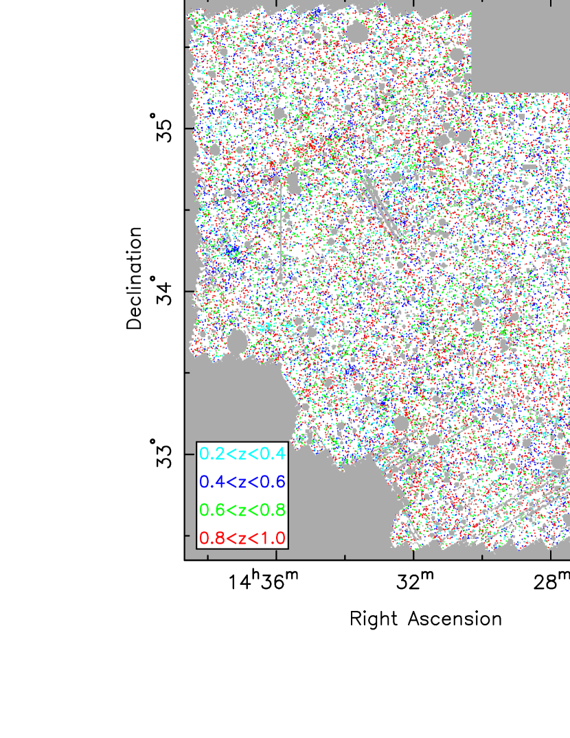
Subsamples are conceptually simple but underestimate the uncertainties, as an individual large-scale structure may span 2 subsamples of the data. For this reason, we only use thirteen $0.5~{}{\rm deg}^{2}$ subsamples rather than many smaller subsamples. For our Schechter function fits we evaluate the luminosity function for each subsample using the method of Marshall et al. (1983) and use the standard deviation of the fitted parameters (e.g., $M^{*}$ ) divided by $\sqrt{13}$ to estimate uncertainties. Luminosity functions for the whole Boötes field and the thirteen subsamples are shown in Figure 9. The subample luminosity functions can differ from the luminosity function for the entire field by as much as $50\%$ . While individual galaxy clusters are evident in Figure 10, these contain but a fraction of all red galaxies and the variations between different subsamples are almost certainly caused by galaxies residing within larger structures.

As the angular correlation function of galaxies does not equal zero on scales of $\sim 1^{\circ}$ , we expect subsamples to underestimate the uncertainties for $\phi^{*}$ and the luminosity density, $j_{B}$ . We do not calculate uncertainties for $M^{*}$ and $\alpha$ using galaxy clustering, as this requires additional information including details of how the shape of the luminosity function varies with galaxy density. The expected variance of the number counts in a field is given by

\left<\frac{n_{i}-<n_{i}>}{n_{i}}\right>^{2}=\frac{1}{<n_{i}>}+\frac{1}{\Omega^{2}}\int\int\omega(\theta)d\Omega_{1}d\Omega_{2}

(5)

(Groth & Peebles 1977; Efstathiou et al. 1991) where $\omega(\theta)$ is the angular correlation function, $\theta$ is the angle separating solid angle elements $d\Omega_{1}$ and $d\Omega_{2}$ , and $\Omega$ is the area of the field. We assume $\omega(\theta)$ is a power-law with index $1-\gamma$ , and use power-law fits to the angular correlation functions from M. J. I. Brown et al. (in preparation). For the Boötes field the sample variance is approximately $n_{i}^{2}\omega(1^{\prime})10^{-1.78(\gamma-1)}$ , while for fields smaller than $1~{}{\rm deg^{2}}$ the sample variance is at least $n_{i}^{2}\omega(1^{\prime})10^{-1.33(\gamma-1)}$ . Table 4 lists uncertainties for $\phi^{*}$ and $j_{B}$ derived from subsamples and the angular clustering, along with the $\omega(1^{\prime})$ and $\gamma$ values from M. J. I. Brown et al. (in preparation). Subsamples underestimate the uncertainties of $\phi^{*}$ and $j_{B}$ by a factor of $\simeq 3$ at low redshift, so throughout the remainder of the paper we use angular clustering uncertainties for $\phi^{*}$ and $j_{B}$ .

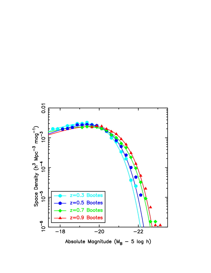
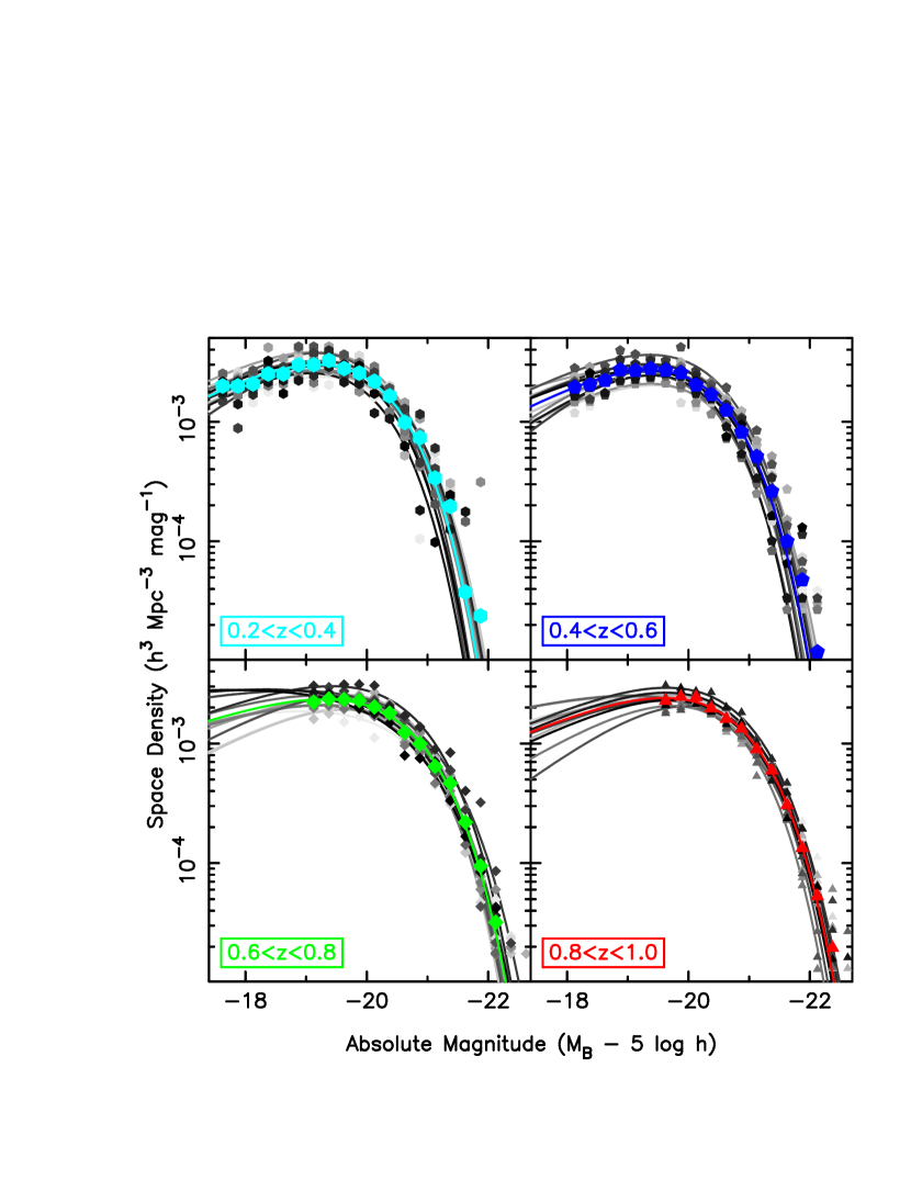
Our $1/V_{max}$ luminosity function values and Schechter function fit parameters are provided in Tables 5 and 6 respectively. For comparison to the prior literature, fits with $\alpha=-0.5$ are also provided in Table 6 though for the remainder of the paper we use fits where $\alpha$ is a free parameter. As shown in Figure 11, Schechter functions provide a good approximation of the observed luminosity function.

It is evident from the fits shown in Figure 11 that the red galaxy luminosity function evolves with redshift. In particular, the bright end of the luminosity function (i.e., at $L\gtrsim L^{*}$ ) steadily fades by $\simeq 0.9$ magnitudes per unit redshift from $z=0.9$ to $z=0.3$ . While $\alpha$ may decrease slightly with increasing redshift, the fits computed for each redshift are constrained by different ranges of galaxy luminosity and the correlation of $\alpha$ with redshift disappears when we only fit the luminosity function of $M_{B}-5{\rm log}h<-19-0.9z$ red galaxies. From Figure 11 and Table 5 it is unclear if the luminosity function is or is not undergoing density evolution. While an apparent decline in the space density is measured (see Table 5), the $1/V_{\rm max}$ luminosity function bins are correlated with each other and Figure 11 does not include the uncertainties from cosmic variance, which are $\simeq 0.1\phi(M)$ . The normalization of the luminosity function, $\phi^{*}$ , also does not show a consistent trend with redshift. We note, however, that $\phi^{*}$ is very sensitive to the measured and assumed values of both $M^{*}$ and $\alpha$ .

In §5.1 and §5.2 we measure the assembly and evolution of red galaxies using the luminosity density and the luminosity evolution of galaxies at a fixed space density threshold. These parameterizations of the evolving luminosity function are not highly correlated with Schechter function parameters such as $\alpha$ . Also, these parameters can be easily compared with simple models of red galaxy assembly and stellar population evolution, thus simplifying the interpretation of the evolving luminosity function of red galaxies.

5.1 THE LUMINOSITY DENSITY AND THE EVOLVING STELLAR MASS WITHIN RED GALAXIES

We use the luminosity density to measure the rest-frame $B$ -band light emitted by ensembles of red galaxies. The luminosity density is strongly correlated with the total stellar mass contained within all red galaxies, though it is also sensitive to the evolving stellar populations of these galaxies. To evaluate the luminosity density for all luminosities, we integrate over the best-fit Schechter functions, so

j_{B}=\phi_{B}^{*}L_{B}^{*}\Gamma(\alpha+2).

(6)

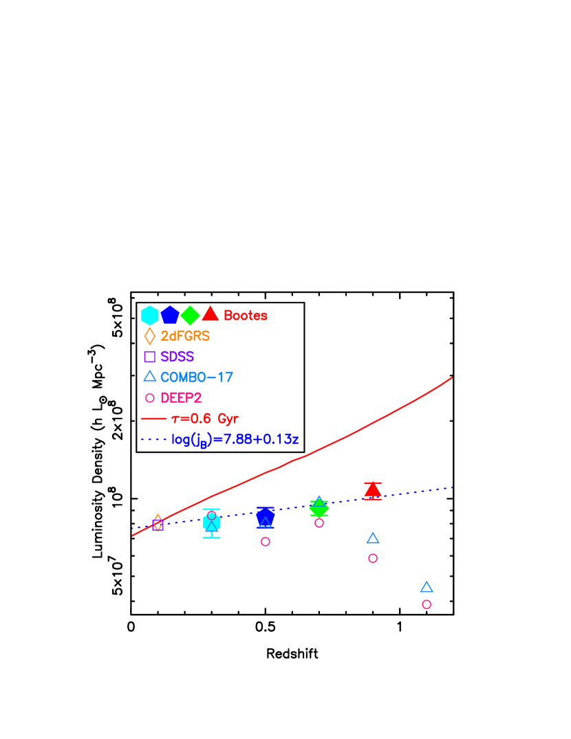
We present the luminosity density of all red galaxies as function of redshift in Figure 12. Luminosity density values are listed in Table 7, including values determined with galaxies brighter than evolving absolute magnitude thresholds which are a function of $M^{*}$ . For our range of $\alpha$ values, less than 25% of the luminosity density is contributed by galaxies fainter than our magnitude limits and approximately 70% of the luminosity density is contributed by galaxies within a magnitude of $M^{*}$ . Our measurements are broadly consistent with the prior literature, except at $z=0.9$ where we find a higher luminosity density than COMBO-17 and DEEP2.

To model the evolution of the luminosity density, we assume that the stellar populations of red galaxies can be approximated by a Bruzual & Charlot (2003) $\tau=0.6~{}{\rm Gyr}$ model with a formation redshift of $z=4$ . This model approximates the evolving rest-frame colors of $M_{V}-5{\rm log}h\sim-21$ red galaxies, which we plot in Figure 4. The $\tau=0.6~{}{\rm Gyr}$ model fades by $1.24$ $B$ -band magnitudes between $z=1$ and $z=0$ , which is consistent with the observed luminosity evolution of both the size-luminosity (Figure 5) and fundamental plane relations (e.g., van Dokkum & Stanford 2003; Treu et al. 2005) of $M_{V}-5{\rm log}h\sim-21$ red galaxies. We caution that less luminous red galaxies are bluer than the $\tau=0.6~{}{\rm Gyr}$ model and their stellar populations may exhibit more rapid luminosity evolution at $z<1$ (e.g., Treu et al. 2005; van der Wel et al. 2005). The $\tau=0.6~{}{\rm Gyr}$ model, normalized to the 2dFGRS, is plotted in Figure 12 and grossly overestimates the evolution of the luminosity density of red galaxies.

The relationship between ${\rm log}(j_{B})$ and redshift in Figure 12 can be approximated by a straight line. If we fit to the Boötes data alone, we find

	$\displaystyle{\rm log}[j_{B}(10^{7}h~{}L_{\odot}~{}{\rm Mpc^{-3}})]$	$\displaystyle=$	$\displaystyle 7.82(\pm 0.06)$
			$\displaystyle+0.22(\pm 0.09)\times z,$

with a reduced $\chi^{2}$ of only $0.2$ . While the $\tau=0.6~{}{\rm Gyr}$ model predicts a $213\%$ increase in the $B$ -band luminosity density of red galaxies between $z=0$ and $z=1$ , using the Boötes data alone we observe an increase of only $65\pm 34\%$ .

Although we have the largest $0.2<z<1.0$ red galaxy sample currently available, our measurement of $j_{B}$ evolution is not sufficiently precise to clearly distinguish between significantly different descriptions of luminosity function evolution: pure luminosity evolution (where $j_{B}$ evolves in the same manner as $L^{*}$ ) or luminosity evolution with up to 50% density evolution between $z=0$ and $z=1$ . While combining data sets can introduce systematic errors, the combined data set allows the investigation of $j_{B}$ over a longer redshift baseline and reduces the random uncertainties at low redshift. The 2dFGRS red galaxy sample is selected using a criterion based upon principal component analysis of 2dF spectra (Madgwick et al. 2002), which is strongly correlated with galaxy rest-frame color. By fitting Bruzual & Charlot (2003) $\tau$ models to galaxies with SDSS photometry and 2dFGRS spectroscopy, we find the 2dF red galaxy selection criterion corresponds to rest-frame $U-V\gtrsim 1.1$ , which is very similar to our criterion for $L^{*}$ red galaxies at low redshift. Using the combined data set, we find

	$\displaystyle{\rm log}[j_{B}(10^{7}h~{}L_{\odot}~{}{\rm Mpc^{-3}})]$	$\displaystyle=$	$\displaystyle 7.88(\pm 0.02)$
			$\displaystyle+0.13(\pm 0.04)\times z,$

which has a reduced $\chi^{2}$ of $0.5$ . Our best fit to the combined data set, shown in Figure 12, yields a $36\pm 13\%$ increase in the luminosity density of red galaxies between $z=0$ and $z=1$ .

We can infer the rate of stellar mass growth within the red galaxy population by comparing the evolution of $j_{B}$ with the luminosity evolution predicted by a stellar population synthesis model. We assume red galaxy stellar populations have faded by $1.24$ $B$ -band magnitudes since $z=1$ , as does the $\tau=0.6~{}{\rm Gyr}$ model. We caution that if we underestimate the luminosity evolution of the stellar populations, we underestimate the growth of stellar mass within red galaxies, and vice versa. If red galaxy stellar populations fade by $1.24$ $B$ -band magnitudes per unit redshift, then using the Boötes data alone we find the stellar mass contained within the red galaxy population has increased by $91\pm 39\%$ since $z=1$ . Using both Boötes and the 2dFGRS, we find the stellar mass contained within the red galaxy population has increased by $131\pm 22\%$ since $z=1$ . Unless we have grossly overestimated the luminosity evolution of red galaxy stellar populations, the stellar mass contained within the red galaxy population has increased by order unity since $z=1$ .

The mild evolution of red galaxy luminosity density rules out several models of red galaxy evolution. Stellar population synthesis models with roughly constant star formation histories exhibit modest evolution of their $B$ -band luminosities at $z<1$ . However, such star formation histories result in galaxies with rest-frame colors of $U-V<0.5$ , which is bluer than any of our red galaxies. While red galaxy mergers occur at $z<1$ (e.g., Lauer 1988; van Dokkum 2005), unless they are accompanied by star formation they will only redistribute stellar mass already within the red galaxy population. Stellar mass must be added to the red galaxy population from an outside source, namely blue galaxies.

Blue galaxies must be adding mass to the red population due to a decline in their star formation rates. Stellar population synthesis models with $1.5~{}{\rm Gyr}<\tau<2.5~{}{\rm Gyr}$ move across our rest-frame $U-V$ selection criterion for $L^{*}$ galaxies between $z=1$ and $z=0$ . Stellar population synthesis models can also move across our selection criterion if star formation is rapidly truncated, possibly after AGN feedback or a merger triggered starburst. While a broad range of star formation histories can transform blue galaxies into red galaxies, the tight color-magnitude relation of red galaxies indicates that red galaxies of a given mass and metallicity have similar low rates of star formation. These galaxies have similar star formation histories over many ${\rm Gyr}$ , or they converge towards similar yet low star formation rates upon entering the red galaxy population. We will explore some of these possibilities in detail in future papers.

5.2 THE EVOLUTION OF VERY LUMINOUS RED GALAXIES

Fading star-forming galaxies cannot explain the evolution of $4L^{*}$ red galaxies at $z<1$ , as star-forming galaxies with comparable masses are exceptionally rare at these redshifts (e.g., Bell et al. 2004). If the stellar mass contained within these very luminous red galaxies is evolving at $z<1$ , this is presumably due to galaxy mergers.

The luminosity density is a poor measure of the evolution of $4L^{*}$ red galaxies. As these galaxies are on the exponential part of the luminosity function, the measured luminosity density and space density of galaxies brighter than an absolute magnitude threshold will have an extremely strong dependence upon that threshold. For example, in Table 7 we list values of $j_{B}$ for $M_{B}<M^{*}-1.5$ galaxies, but $M^{*}$ is correlated with $\alpha$ so the $j_{B}$ values determined with floating and fixed values of $\alpha$ differ by up to $35\%$ . Similarly, if the measured luminosities or the assumed luminosity evolution of $4L^{*}$ red galaxies are in error 0.1 magnitudes, the measured space density evolution of red galaxies can be in error by 30%. If the stellar populations of today’s $L^{*}$ and $4L^{*}$ galaxies did not evolve in the same manner, luminosity density values derived with $M_{B}<M^{*}-1.5$ red galaxies can provide a misleading picture of $4L^{*}$ red galaxy evolution.

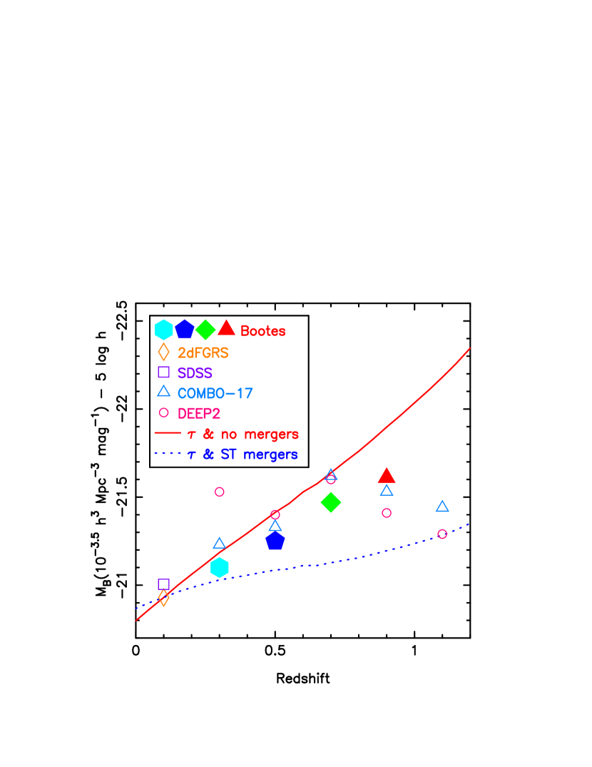
We avoid these issues by measuring the evolving luminosity function at a fixed space density threshold. We parameterize the luminosity evolution with $M(10^{-3.5})$ , the absolute magnitude where the space density of red galaxies is $10^{-3.5}~{}h^{-3}~{}{\rm Mpc}^{-3}~{}{\rm mag}^{-1}$ . The most luminous red galaxies largely lie along the color magnitude relation, so $M(10^{-3.5})$ is insensitive to details of red galaxy selection criteria and it is thus easy to compare the results of various surveys. Schechter functions provide a good fit to the red galaxy luminosity function when the space density is above $10^{-4.5}~{}h^{-3}~{}{\rm Mpc}^{-3}~{}{\rm mag}^{-1}$ (e.g., Madgwick et al. 2002), so we use best-fit Schechter functions to derive $M(10^{-3.5})$ from our data and the literature (when available). Our estimates of $M(10^{-3.5})$ are provided in Table 6, and plotted in Figure 13 along with values derived from the literature. We find $M_{B}(10^{-3.5})$ steadily increases with increasing redshift. A straight line fit to the Boötes data alone has a reduced $\chi^{2}$ of $1.1$ and $M_{B}(10^{-3.5})$ brightens by $0.87\pm 0.06$ $B$ -band magnitudes from $z=0$ to $z=1$ . While there are some discrepancies between the surveys at $z\sim 0.9$ , which we discuss in §6, there is broad agreement between our results and the literature at $z<0.8$ . If we fit to both the Boötes and 2dFGRS data, we find $M(10^{-3.5})$ brightens by $0.87\pm 0.05$ $B$ -band magnitudes between $z=0$ and $z=1$ .

We use two simple models to characterize the evolution of $M_{B}(10^{-3.5})$ . Both models are intended to be illustrative rather than precise descriptions of galaxy evolution. Our simplest model has no galaxy mergers and assumes that the star formation history of all red galaxy progenitors is described by a Bruzual & Charlot (2003) $\tau=0.6~{}{\rm Gyr}$ model. This $\tau$ model has negligible star formation at $z<1$ and approximates the evolution of the color-magnitude and size-luminosity relations of $\sim 4L^{*}$ red galaxies (Figures 4 and 5). As mergers of red galaxies do occur at $z<1$ (e.g., Lauer 1988; van Dokkum 2005), this model provides an upper bound for the fading of $M_{B}(10^{-3.5})$ from $z=1$ to $z=0$ .

Our second model of $M_{B}(10^{-3.5})$ assumes galaxy mergers can be described by the Sheth & Tormen (1999) halo mass function, which is similar to the formalism of Press & Schechter (1974). We assume one galaxy per dark matter halo, a constant ratio of baryonic matter to dark matter in each halo, and a $\tau=0.6~{}{\rm Gyr}$ model star formation history. From the halo mass function we can determine the space density of halos more massive than $m_{min}$ , and we know the space density of galaxies brighter than $M_{B}(10^{-3.5})$ is $\simeq 10^{-4}h^{3}{\rm Mpc}^{-3}$ . We therefore assume that the growth of baryons within $M_{B}(10^{-3.5})$ galaxies is proportional to the evolving $m_{min}$ value corresponding to a halo space density of $10^{-4}h^{3}{\rm Mpc}^{-3}$ . We find $m_{min}>10^{13}M_{\odot}$ at $z<1$ , which is comparable to the masses of galaxy groups. This simple model is clearly flawed, as group and cluster halos contain multiple galaxies, and the infall of galaxies into these halos may not result in galaxy mergers. As this model overestimates the rate of galaxy mergers, it should provide a lower bound for the evolution of $M_{B}(10^{-3.5})$ .

Our $M_{B}(10^{-3.5})$ models are plotted in Figure 13, along with $M_{B}(10^{-3.5})$ values derived from this work and the literature. The model without mergers clearly provides the better approximation to the data. This model is offset from the data by only $0.21$ magnitudes at $z=0.7$ and $0.31$ magnitudes at $z=0.9$ . If the stellar populations of red galaxies fade in the same manner as the $\tau=0.6~{}{\rm Gyr}$ model, $\simeq 75\%$ of the stellar mass contained within today’s $4L^{*}$ galaxies was already in place within these galaxies by $z=0.9$ . If red galaxy stellar populations fade by less than $1.24$ $B$ -band magnitudes from $z=1$ to $z=0$ , an even higher percentage of the stellar mass of $4L^{*}$ red galaxies is already in place prior to $z=0.9$ , and vice versa. While we measure a higher space density of very luminous red galaxies at $z=0.9$ than the literature, there is broad agreement at lower redshifts. Even if the Boötes measurements at $z=0.9$ are in error, the space density of $4L^{*}$ red galaxies from the literature is approximated by our model at $z\leq 0.7$ . Roughly 80% of the stellar mass within today’s $4L^{*}$ red galaxies must already be in place by $z=0.7$ .

We can see in Figure 13 that the simple merging model, based upon the Sheth & Tormen (1999) halo mass function for a $\Lambda{\rm CDM}$ cosmology, differs significantly from the observed evolution of $M(10^{-3.5})$ . The simplifying assumptions used in this model may explain the offset from the data. We assumed one galaxy per halo, while the most luminous red galaxies often reside within galaxy groups and clusters. An accurate model of these galaxies requires a description of how these galaxies occupy subhalos within groups and clusters, and how these subhalos merge over cosmic time. Such a model must also have negligible star formation at $z<1$ , and clearly there is a physical process that is extremely effective at truncating star formation in $4L^{*}$ red galaxies. Issues such as the halo occupation distribution function (e.g., Berlind & Weinberg 2002), gas heating (e.g., Naab et al. 2005), and AGN feedback (e.g., Bower et al. 2006; Croton et al. 2006; Hopkins et al. 2006) are clearly important for understanding galaxy evolution and need to be studied in more detail.

6 COMPARISON TO OTHER RED GALAXY LUMINOSITY FUNCTIONS

There have been a variety of conclusions about red galaxy evolution over the past decade (see Faber et al. 2005), and some of this can be explained by the different behavior of $L^{*}$ and $4L^{*}$ red galaxies (§5.1 and §5.2 respectively). Bundy et al. (2005) also find that the evolution of red galaxies is a function of stellar mass, and this has been confirmed by recent analyzes of COMBO-17 stellar mass and luminosity functions (Borch et al. 2006; Cimatti, Daddi, & Renzini 2006). The luminosity density of red galaxies is heavily weighted towards $L^{*}$ galaxies and evolves slowly at $z<1$ . After accounting for fading stellar populations, we and much of the recent literature (e.g., Bell et al. 2004; Faber et al. 2005) conclude that the stellar mass contained within the ensemble of red galaxies has steadily increased since $z=1$ . In contrast, the evolution of $4L^{*}$ red galaxies differs only slightly from pure luminosity evolution. However, unlike some recent studies (e.g., Bundy et al. 2005; Borch et al. 2006; Cimatti et al. 2006), we do see evidence for the ongoing assembly of the most massive red galaxies, albeit at a rate that produces little growth of $4L^{*}$ red galaxy stellar masses at $z<1$ . As red galaxy evolution is a function of luminosity, it is not surprising that various authors using different techniques have reached a variety of conclusions, even when using the same galaxy surveys (e.g., Bell et al. 2004; Willmer et al. 2005; Faber et al. 2005; Blanton 2005; Bundy et al. 2005; Borch et al. 2006; Cimatti et al. 2006).

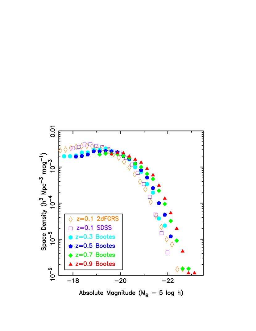
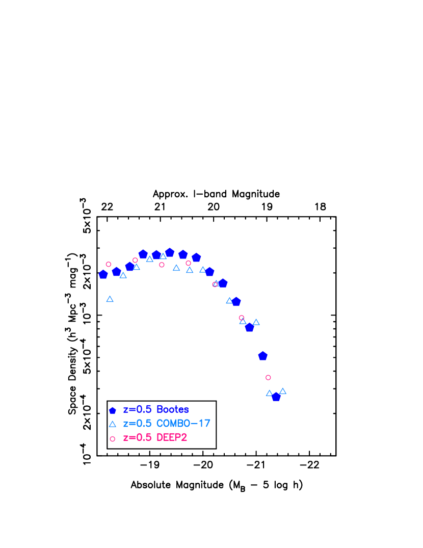
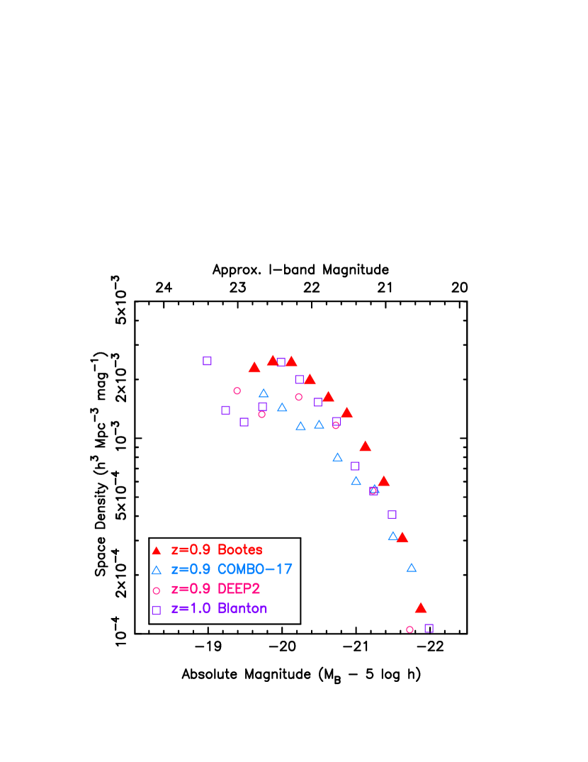
Figures 14 and 15 show our evolving luminosity functions are broadly consistent with the 2dFGRS, SDSS, COMBO-17 and DEEP2 at $z\lesssim 0.8$ . There is a steady increase of the bright end of the luminosity function with redshift. If we combine our results with those of the 2dFGRS and SDSS, there is a gradual decline of $\phi^{*}$ with increasing redshift. However, we show in Figure 15 that we measure a higher space density of $z=0.9$ red galaxies than DEEP2 or COMBO-17. Since these studies have had a significant impact upon the field, it is important to understand why these differences occur.

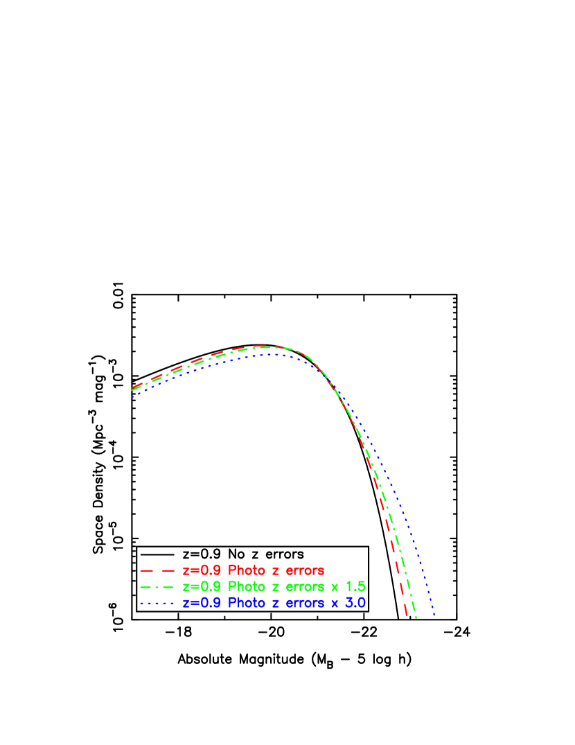
An obvious difference between our work and some of the recent literature is our use of photometric redshifts. Photometric redshift errors can scatter numerous low luminosity objects into high luminosity bins, and thus alter the shape of the luminosity function (e.g., Brown, Webster, & Boyle 2001; Chen et al. 2003). To account for this we convolved our evolving luminosity function by the expected luminosity and volume errors resulting from our photometric redshifts. We use the photometric redshift errors listed in Table 1, except at faint magnitudes with ten or less spectroscopic redshifts, where we extrapolate from brighter magnitudes by assuming the errors increase by 50% per unit magnitude. In Figure 16 the largest error is a $\simeq 0.2$ magnitude offset for rare $10L^{*}$ galaxies at $z=0.9$ . In Figure 11, there are slightly more $10L^{*}$ galaxies than expected from our best-fit $z=0.9$ Schechter function, but these are a tiny fraction of our sample and do not affect our results, which rely upon less luminous galaxies.

Compared to the other luminosity functions in Table 6, the VIRMOS-VLT Deep Survey (VVDS; Zucca et al. 2005) find a lower space density of high redshift and low luminosity red galaxies. As discussed by Zucca et al. (2005), this is not unexpected as the VVDS selection criteria do not model the evolution and tilt of the color-magnitude relation. Wolf et al. (2003) also observed a rapid decline of $\phi^{*}$ with redshift for a sample of red galaxies selected from COMBO-17 with a non-evolving criterion. Similar selection effects may occur in other surveys by accident at $z>1$ , where the evolving color-magnitude relation is relatively difficult to measure and red galaxy selection criteria could unintentionally intercept the color-magnitude relation.

Both the VVDS and COMBO-17 use SExtractor MAG_AUTO to determine total magnitudes, and accuracy of the SDSS DR1 and 2dFGRS photometry has been verified with deep CCD photometry making use of MAG_AUTO (Cross et al. 2004). MAG_AUTO is known to underestimate the luminosities of galaxies with de Vaucouleurs (1948) profiles by $0.1$ magnitudes when the half-light radius is several times larger than the stellar full width at half maximum (Cross et al. 2004). It is therefore plausible that the brightest red galaxies in the 2dFGRS have had their luminosities underestimated by $\sim 10\%$ . As illustrated in Figure 1, MAG_AUTO can also have systematics of several tenths of a magnitude at $I>21$ , even when the catalogs are 85% complete. We therefore speculate that the VVDS and COMBO-17 may have systematic errors on the order of $0.2$ magnitudes at the faint end of their luminosity functions.

While our $z\simeq 0.9$ luminosity functions and those derived from DEEP2 (Willmer et al. 2005; Faber et al. 2005; Blanton 2005) are broadly similar in shape and normalization, there is a systematic offset of $\simeq 0.2$ magnitudes. This offset is present even at high luminosities, which are largely insensitive to the selection effects discussed elsewhere in this paper. As discussed in §3.4, we correct for flux outside of our aperture using a model derived from the size-luminosity relation. Such corrections are typically not applied to samples in the literature.

We have estimated the fraction of galaxy flux that falls beyond the photometric aperture used by the DEEP2 survey. DEEP2 photometry uses the larger of a $2^{\prime\prime}$ diameter aperture or a $6\sigma$ aperture, where $\sigma$ is defined by a Gaussian fit to the object profile (Coil et al. 2004). DEEP2 photometry is zero-pointed with SDSS photometry of stars, where the SDSS uses PSF magnitudes while DEEP2 uses apertures of $\simeq 2^{\prime\prime}$ diameter. Because of this, a point source measured with a $>2^{\prime\prime}$ diameter aperture will have its flux systematically overestimated. Similarly, the photometry of galaxies will have systematic errors which are a function of half-light radius and aperture size. In Figure 17, we plot the DEEP2 aperture diameter as a function of apparent magnitude for $0.8<z<1.0$ red galaxies selected from the first DEEP2 data release. At these redshifts, an $I\sim 21.5$ galaxy has a half-light radius of $\simeq 0.5^{\prime\prime}$ ( $\simeq 3h^{-1}{\rm kpc}$ ), and we list the systematic error for such a galaxy measured with the DEEP2 aperture on the right of Figure 17. Red galaxies at $z\sim 0.9$ may have their luminosities systematically underestimated by $\simeq 0.15$ magnitudes by DEEP2, and we therefore conclude that different measures of total magnitudes contribute to the difference between our work and the prior literature.

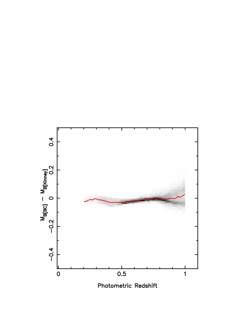
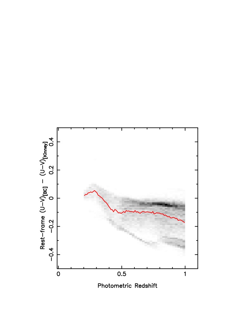
Different surveys use different SED models and templates to derive rest-frame galaxy properties from observed photometry. Figure 18 compares rest-frame magnitudes and colors derived with the Bruzual & Charlot (2003) $\tau$ models and Kinney et al. (1996) templates for our red galaxy sample. The absolute magnitudes exhibit small differences, as the observed $I$ -band is very close to the rest-frame $B$ -band at $z=0.9$ . In contrast, the rest-frame $U-V$ colors show systematics as large as 0.2 magnitudes. This will have minimal impact on the bright end of the luminosity function, as the most luminous red galaxies lie along the color-magnitude relation, which can be identified empirically. The greatest impact from SED errors will be at lower luminosities, as SED errors will shift red galaxy selection criterion relative to the the color-magnitude relation. A $0.1$ magnitude shift in our $U-V$ selection criterion results in our $\phi^{*}$ and $j_{B}$ values changing by $\sim 25\%$ .

If the Kinney et al. (1996) templates are better models of $z\sim 0.9$ red galaxy SEDs than the Bruzual & Charlot (2003) $\tau$ models, our principal conclusions remain unchanged. The $U-V$ color-magnitude relation still evolves, but the mean color and luminosity of red galaxy stellar populations evolves less rapidly than predicted by the $\tau=0.6~{}{\rm Gyr}$ model. Even if our $z=0.9$ $j_{B}$ measurement has a $25\%$ error, the stellar mass contained within the red galaxy population must increase with decreasing redshift. If we reduce the luminosity evolution of red galaxy stellar populations, a revised $M_{B}(10^{-3.5})$ model without mergers will provide a better fit to the observations in Figure 13 than our current model.

7 SUMMARY

We have measured the evolution and assembly of red galaxies over the last $8~{}{\rm Gyr}$ , using the evolving $B$ -band luminosity function of $0.2<z<1.0$ red galaxies. Our sample of 39599 $0.2<z<1.0$ red galaxies, selected from $6.96~{}{\rm deg}^{2}$ of imaging, is an order of magnitude larger in size and volume than comparable $z\sim 0.9$ red galaxy samples. Accurate photometric redshifts were determined using the empirical ANNz photometric redshift code and photometry from both the NOAO Deep Wide-Field and Spitzer IRAC shallow surveys. The accuracy of these redshifts has been verified with spectroscopy, and is comparable to the best broad-band photometric redshifts in the literature.

We find the color-magnitude and size-luminosity relations of red galaxies evolve with redshift, and this evolution can be approximated by a Bruzual & Charlot (2003) $\tau=0.6~{}{\rm Gyr}$ stellar population synthesis model. The size-luminosity relation predicts a significant fraction of the galaxy flux is at radii of several arcseconds, even at $z\sim 0.9$ . Luminosity functions which do not account for this underestimate the space density of red galaxies at high redshift, and overestimate the assembly rate of red galaxies at $z<1$ .

We find the luminosity density, $j_{B}$ , of red galaxies increases by $36\pm 13\%$ from $z=0$ to $z=1$ . In contrast, the $B$ -band luminosity of a $\tau=0.6~{}{\rm Gyr}$ stellar population model increases by 213% over the same redshift range. If red galaxy stellar populations fade by $1.24$ magnitudes from $z=1$ to $z=0$ , the stellar mass contained within red galaxies has approximately doubled over the past $8~{}{\rm Gyr}$ . Blue galaxies are being transformed into $\lesssim L^{*}$ red galaxies at $z<1$ , after a steady decline or rapid truncation of their star formation.

The evolution of the most luminous red galaxies at $z<1$ cannot be dominated by fading blue galaxies, as blue galaxies with large stellar masses are exceptionally rare at $z<1$ . We have measured the evolution of $4L^{*}$ red galaxies using $M_{B}(10^{-3.5})$ , the absolute magnitude corresponding to a fixed space density of $10^{-3.5}~{}h^{3}~{}{\rm Mpc^{-3}}~{}{\rm mag^{-1}}$ . Our measurements of $M_{B}(10^{-3.5})$ , along with those we derived from the literature, show that the stellar masses of the most luminous red galaxies evolve slowly at $z<1$ . A Bruzual & Charlot (2003) $\tau=0.6~{}{\rm Gyr}$ model, with little stellar mass evolution and normalized to the 2dFGRS, only overestimates $M_{B}(10^{-3.5})$ by $\simeq 0.21$ magnitudes at $z=0.7$ . We therefore conclude that $\simeq 80\%$ of the stellar mass contained within today’s $M_{B}-5{\rm log}h=-21$ red galaxies was already in place within these galaxies at $z=0.7$ . While red galaxy mergers have been reported in the prior literature, such mergers do not rapidly increase the stellar masses of $4L^{*}$ red galaxies between $z=1$ and the present day.

We thank our colleagues on the NDWFS, IRAC Shallow Survey, and AGES teams, in particular R. J. Cool, D. J. Eisenstein, G. G. Fazio, C. S. Kochanek, S. S. Murray, and G. P. Tiede. This paper would not have been possible without the efforts of the KPNO, Spitzer, MMT, W. M. Keck and Gemini support staff. We are grateful to the IRAF team for the majority of the packages used to process the NDWFS images. We thank Alyson Ford, Lissa Miller, and Jennifer Claver, for reducing much of the NDWFS data used for this paper. H. Spinrad, S. Dawson, D. Stern, J. E. Rhoads, S Malhotra, B. T. Soifer, C. Bian, S. G. Djorgovski, S. A. Stanford, S. Croft, W. van Breugel and the AGES collaboration generously shared their spectroscopic redshifts with us prior to publication. This work is based in part on observations made with the Spitzer Space Telescope, which is operated by the Jet Propulsion Laboratory, California Institute of Technology under a contract with NASA. This research was supported by the National Optical Astronomy Observatory which is operated by the Association of Universities for Research in Astronomy (AURA), Inc. under a cooperative agreement with the National Science Foundation. Most of the spectroscopic redshifts discussed in this paper were obtained at the MMT Observatory, a joint facility of the Smithsonian Institution and the University of Arizona. While writing this paper we had many productive discussions with other astronomers working upon galaxy assembly and evolution, including E. F. Bell, M. R. Blanton, A. L. Coil, S. M. Faber, J. .E. Gunn, T. R. Lauer, J. A. Newman, J. P. Ostriker, C. N. A. Willmer, C. Wolf, and E. Zucca.

Table 1: Measured Photometric Redshift Uncertainties For Red Galaxies

	$0.2<z<0.4$			$0.4<z<0.6$			$0.6<z<0.8$			$0.8<z<1.0$
$4^{\prime\prime}$ Apparent	$M_{B}-5{\rm log}h<-17.5$			$M_{B}-5{\rm log}h<-18.0$			$M_{B}-5{\rm log}h<-19.0$			$M_{B}-5{\rm log}h<-19.5$
Magnitude	68.7%	90%	$N$	68.7%	90%	$N$	68.7%	90%	$N$	68.7%	90%	$N$
$17.0<I<18.0$	0.033	0.060	$(170)$	–	–	–	–	–	–	–	–	–
$18.0<I<19.0$	0.032	0.063	$(1110)$	0.026	0.051	$(132)$	0.025	0.025	$(1)$	–	–	–
$19.0<I<20.0$	0.039	0.074	$(1007)$	0.032	0.058	$(949)$	0.029	0.053	$(192)$	0.027	0.179	$(10)$
$20.0<I<21.0$	0.049	0.088	$(166)$	0.036	0.066	$(340)$	0.040	0.072	$(240)$	0.058	0.096	$(50)$
$21.0<I<22.0$	0.042	0.363	$(4)$	0.229	3.066	$(5)$	0.103	0.131	$(14)$	0.045	0.090	$(28)$
$22.0<I<23.5$	–	–	–	–	–	–	0.162	0.271	$(5)$	0.127	0.254	$(7)$

Table 2: Color cuts used to exclude stars, quasars and

z\gg 1

galaxies from the sample.

Magnitude and/or color range	Cut
$B_{W}\leq 26.5$	$B_{W}-R<1.00$
$B_{W}\leq 26.5$	$B_{W}-R>4.20$
$B_{W}>26.5$	$26.5-R>4.20$
$B_{W}\leq 26.5$	$B_{W}-R>2.55+2.75\times(R-I-0.55)$
$B_{W}>26.5$	$26.5-R>2.55+2.75\times(R-I-0.55)$
$I<23.5$	$R-I<0.55$
$I<23.5$	$R-I>1.70$
$B_{W}\leq 26.5$	$B_{W}-R<2.0-(R-I)$
$B_{W}\leq 26.5$	$B_{W}-R<5.0\times(R-I-1.2)$
$[3.6]\leq 19.5$	$I-[3.6]<2.2$
$[3.6]>19.5$	$I-19.5<2.2$
$[3.6]\leq 19.5$ and $0.75\leq R-I<1.05$	$R-I>0.75+0.375\times(I-[3.6]-2.2)$
$[3.6]>19.5$ and $0.75\leq R-I<1.05$	$R-I>0.75+0.375\times(I-19.5-2.2)$
$[3.6]\leq 19.5$ and $1.05\leq R-I<1.70$	$R-I>1.05+0.60\times(I-[3.6]-3.0)$
$[3.6]>19.5$ and $1.05\leq R-I<1.70$	$R-I>1.05+0.60\times(I-19.5-3.0)$
$[3.6]\leq 19.5$ and $[3.6]\leq 18.5$	$[3.6]-[4.5]>0.6$
$[3.6]\leq 19.5$ and $[3.6]\leq 18.5$	$[3.6]-[4.5]<-0.6$

Table 3: Red Galaxy Number Counts

$4^{\prime\prime}$ Apparent	$0.2<z<0.4$	$0.4<z<0.6$	$0.6<z<0.8$	$0.8<z<1.0$
Magnitude	$M_{B}-5{\rm log}h<-17.5$	$M_{B}-5{\rm log}h<-18.0$	$M_{B}-5{\rm log}h<-19.0$	$M_{B}-5{\rm log}h<-19.5$
$17.0<I<18.0$	189	—–	—–	—–
$18.0<I<19.0$	1272	141	1	—–
$19.0<I<20.0$	2365	2131	400	14
$20.0<I<21.0$	1719	4591	3320	977
$21.0<I<22.0$	438	3512	5738	5466
$22.0<I<23.5$	—–	608	1359	5358

Table 4: Comparison of subsample and clustering uncertainties for

\phi^{*}

and

j_{B}

$z$ range	$\omega(1^{\prime})$	$\gamma$	$\phi^{*}\times 10^{2}(h^{3}{\rm Mpc^{-3}~{}mag^{-1}})$			$j_{B}(10^{7}h~{}L_{\odot}~{}{\rm Mpc^{-3}})$
			Best fit	Subsample	Clustering	Best fit	Subsample	Clustering
			Value	$1\sigma$	$1\sigma$	Value	$1\sigma$	$1\sigma$
$0.20<z<0.40$	$0.74\pm 0.05$	$1.94\pm 0.05$	$8.45$	$\pm 0.38$	$\pm 1.07$	$8.1$	$\pm 0.3$	$\pm 1.0$
$0.40<z<0.60$	$0.51\pm 0.03$	$2.02\pm 0.07$	$7.61$	$\pm 0.34$	$\pm 0.68$	$8.5$	$\pm 0.4$	$\pm 0.8$
$0.60<z<0.80$	$0.28\pm 0.02$	$2.06\pm 0.06$	$5.71$	$\pm 0.33$	$\pm 0.35$	$9.2$	$\pm 0.4$	$\pm 0.6$
$0.80<z<1.00$	$0.24\pm 0.02$	$1.93\pm 0.05$	$6.35$	$\pm 0.21$	$\pm 0.47$	$10.7$	$\pm 0.3$	$\pm 0.8$

Table 5: Red Galaxy

1/V_{max}

Luminosity Function with subsample uncertainties

Absolute	Luminosity Function ( $h^{3}~{}{\rm Mpc^{-3}~{}mag^{-1}}$ )
Magnitude	$0.2<z<0.4$	$0.4<z<0.6$	$0.6<z<0.8$	$0.8<z<1.0$
$-17.75<M_{B}-5{\rm log}h<-17.50$	$1.99\pm 0.10\times 10^{-3}$	-	-	-
$-18.00<M_{B}-5{\rm log}h<-17.75$	$1.99\pm 0.13\times 10^{-3}$	-	-	-
$-18.25<M_{B}-5{\rm log}h<-18.00$	$2.07\pm 0.10\times 10^{-3}$	$1.94\pm 0.12\times 10^{-3}$	-	-
$-18.50<M_{B}-5{\rm log}h<-18.25$	$2.51\pm 0.18\times 10^{-3}$	$2.03\pm 0.13\times 10^{-3}$	-	-
$-18.75<M_{B}-5{\rm log}h<-18.50$	$2.51\pm 0.13\times 10^{-3}$	$2.21\pm 0.11\times 10^{-3}$	-	-
$-19.00<M_{B}-5{\rm log}h<-18.75$	$2.98\pm 0.17\times 10^{-3}$	$2.71\pm 0.16\times 10^{-3}$	-	-
$-19.25<M_{B}-5{\rm log}h<-19.00$	$3.00\pm 0.17\times 10^{-3}$	$2.68\pm 0.13\times 10^{-3}$	$2.22\pm 0.11\times 10^{-3}$	-
$-19.50<M_{B}-5{\rm log}h<-19.25$	$3.25\pm 0.18\times 10^{-3}$	$2.78\pm 0.11\times 10^{-3}$	$2.36\pm 0.11\times 10^{-3}$	-
$-19.75<M_{B}-5{\rm log}h<-19.50$	$2.78\pm 0.14\times 10^{-3}$	$2.69\pm 0.10\times 10^{-3}$	$2.34\pm 0.11\times 10^{-3}$	$2.27\pm 0.08\times 10^{-3}$
$-20.00<M_{B}-5{\rm log}h<-19.75$	$2.55\pm 0.14\times 10^{-3}$	$2.56\pm 0.18\times 10^{-3}$	$2.29\pm 0.10\times 10^{-3}$	$2.46\pm 0.10\times 10^{-3}$
$-20.25<M_{B}-5{\rm log}h<-20.00$	$2.17\pm 0.14\times 10^{-3}$	$2.03\pm 0.12\times 10^{-3}$	$2.02\pm 0.14\times 10^{-3}$	$2.44\pm 0.07\times 10^{-3}$
$-20.50<M_{B}-5{\rm log}h<-20.25$	$1.64\pm 0.08\times 10^{-3}$	$1.68\pm 0.07\times 10^{-3}$	$1.80\pm 0.06\times 10^{-3}$	$1.97\pm 0.07\times 10^{-3}$
$-20.75<M_{B}-5{\rm log}h<-20.50$	$9.87\pm 0.76\times 10^{-4}$	$1.24\pm 0.09\times 10^{-3}$	$1.24\pm 0.08\times 10^{-3}$	$1.61\pm 0.07\times 10^{-3}$
$-21.00<M_{B}-5{\rm log}h<-20.75$	$7.35\pm 0.96\times 10^{-4}$	$8.16\pm 0.67\times 10^{-4}$	$9.95\pm 0.65\times 10^{-4}$	$1.33\pm 0.07\times 10^{-3}$
$-21.25<M_{B}-5{\rm log}h<-21.00$	$3.37\pm 0.47\times 10^{-4}$	$5.12\pm 0.46\times 10^{-4}$	$6.44\pm 0.34\times 10^{-4}$	$8.97\pm 0.46\times 10^{-4}$
$-21.50<M_{B}-5{\rm log}h<-21.25$	$1.96\pm 0.22\times 10^{-4}$	$2.62\pm 0.37\times 10^{-4}$	$4.66\pm 0.41\times 10^{-4}$	$5.94\pm 0.25\times 10^{-4}$
$-21.75<M_{B}-5{\rm log}h<-21.50$	$3.76\pm 2.03\times 10^{-5}$	$1.00\pm 0.19\times 10^{-5}$	$2.20\pm 0.22\times 10^{-4}$	$3.06\pm 0.22\times 10^{-4}$
$-22.00<M_{B}-5{\rm log}h<-21.75$	$2.38\pm 2.41\times 10^{-5}$	$4.76\pm 1.09\times 10^{-5}$	$9.47\pm 1.97\times 10^{-5}$	$1.34\pm 0.14\times 10^{-4}$
$-22.25<M_{B}-5{\rm log}h<-22.00$	-	$1.19\pm 0.45\times 10^{-5}$	$3.21\pm 0.63\times 10^{-5}$	$5.30\pm 0.74\times 10^{-5}$
$-22.50<M_{B}-5{\rm log}h<-22.25$	-	$<1.78\times 10^{-5}$	$9.16\pm 3.08\times 10^{-6}$	$1.96\pm 0.54\times 10^{-5}$
$-22.75<M_{B}-5{\rm log}h<-22.50$	-	$<2.20\times 10^{-5}$	$1.53\pm 1.35\times 10^{-6}$	$4.61\pm 2.42\times 10^{-6}$
$-23.00<M_{B}-5{\rm log}h<-22.75$	-	$<3.02\times 10^{-5}$	$1.53\pm 1.61\times 10^{-6}$	$1.15\pm 1.03\times 10^{-6}$

Table 6: Recent

B

-band luminosity functions of red galaxies

Survey^a^aBoötes (this work), 2dFGRS (2dF Galaxy Redshift Survey; Madgwick et al. 2002), COMBO-17 (Classifying Objects by Medium-Band Observations - a spectrophotometric 17-filter survey; Bell et al. 2004; Faber et al. 2005), DEEP2 (Deep Extragalactic Evolution Probe 2; Willmer et al. 2005; Faber et al. 2005), VVDS (VIRMOS-VLT Deep Survey; Zucca et al. 2005)	$z$ range	$N_{galaxy}$	$M^{*}_{B}-5{\rm log}h$ ^b^bWe have adopted $B_{J}-B=0.15$ and $B_{\rm Vega}=B_{\rm AB}$ . Uncertainties are as published and may not account for the contribution of large-scale structure.	$M_{B}(10^{-3.5})-5{\rm log}h$ ^c^cWe have not determined uncertainties for other surveys, but uncertainties for $M(10^{-3.5}h^{3}~{}{\rm Mpc^{-3}~{}mag^{-1}})$ are probably comparable to those for $M^{*}$	$\phi^{*}(h^{3}{\rm Mpc^{-3}~{}mag^{-1}})$	$\alpha$ ^d^dValues of $\alpha$ without uncertainties denote Schechter function fits where $\alpha$ was fixed.
Boötes	$0.20<z<0.40$	5983	$-19.54\pm 0.05$	$-21.10\pm 0.03$	$8.45\pm 1.07\times 10^{-3}$	$-0.28\pm 0.04$
Boötes	$0.40<z<0.60$	10983	$-19.72\pm 0.04$	$-21.25\pm 0.03$	$7.61\pm 0.68\times 10^{-3}$	$-0.28\pm 0.05$
Boötes	$0.60<z<0.80$	10817	$-20.16\pm 0.05$	$-21.47\pm 0.02$	$5.71\pm 0.35\times 10^{-3}$	$-0.55\pm 0.06$
Boötes	$0.80<z<1.00$	11816	$-20.21\pm 0.03$	$-21.61\pm 0.02$	$6.35\pm 0.47\times 10^{-3}$	$-0.43\pm 0.05$
Boötes	$0.20<z<0.40$	5983	$-19.78\pm 0.02$	$-21.19\pm 0.03$	$7.16\pm 0.90\times 10^{-3}$	$-0.50$
Boötes	$0.40<z<0.60$	10983	$-19.92\pm 0.02$	$-21.30\pm 0.03$	$6.60\pm 0.59\times 10^{-3}$	$-0.50$
Boötes	$0.60<z<0.80$	10817	$-20.12\pm 0.02$	$-21.46\pm 0.02$	$5.87\pm 0.36\times 10^{-3}$	$-0.50$
Boötes	$0.80<z<1.00$	11816	$-20.26\pm 0.01$	$-21.62\pm 0.02$	$6.17\pm 0.45\times 10^{-3}$	$-0.50$
2dFGRS	$z<0.15$	27540	$-19.43\pm 0.05$	$-20.93$	$9.9\pm 0.5\times 10^{-3}$	$-0.54\pm 0.02$
COMBO-17	$0.2<z<0.4$	1096	$-19.86\pm 0.16$	$-21.23$	$6.38\pm 2.47\times 10^{-3}$	$-0.50$
COMBO-17	$0.4<z<0.6$	1179	$-20.00\pm 0.11$	$-21.33$	$5.82\pm 0.94\times 10^{-3}$	$-0.50$
COMBO-17	$0.6<z<0.8$	1431	$-20.33\pm 0.12$	$-21.62$	$5.17\pm 0.20\times 10^{-3}$	$-0.50$
COMBO-17	$0.8<z<1.0$	892	$-20.41\pm 0.14$	$-21.53$	$3.46\pm 0.15\times 10^{-3}$	$-0.50$
COMBO-17	$1.0<z<1.2$	256	$-20.81\pm 0.16$	$-21.44$	$1.55\pm 0.34\times 10^{-3}$	$-0.50$
DEEP2	$0.2<z<0.4$	109	$-20.25\pm 0.18$	$-21.53$	$4.97\pm 0.48\times 10^{-3}$	$-0.50$
DEEP2	$0.4<z<0.6$	173	$-20.20\pm 0.12$	$-21.40$	$4.13\pm 0.19\times 10^{-3}$	$-0.50$
DEEP2	$0.6<z<0.8$	196	$-20.42\pm 0.06$	$-21.60$	$3.98\pm 0.31\times 10^{-3}$	$-0.50$
DEEP2	$0.8<z<1.0$	535	$-20.34\pm 0.05$	$-21.41$	$3.13\pm 0.11\times 10^{-3}$	$-0.50$
DEEP2	$1.0<z<1.2$	178	$-20.67\pm 0.08$	$-21.29$	$1.58\pm 0.25\times 10^{-3}$	$-0.50$
VVDS	$0.2<z<0.4$	65	$-20.27\pm^{0.27}_{0.31}$	$-21.66$	$5.15\pm 0.64\times 10^{-3}$	$-0.29$
VVDS	$0.4<z<0.6$	106	$-20.49\pm^{0.17}_{0.18}$	$-21.67$	$3.12\pm 0.30\times 10^{-3}$	$-0.29$
VVDS	$0.6<z<0.8$	197	$-20.22\pm^{0.09}_{0.10}$	$-21.46$	$3.53\pm 0.35\times 10^{-3}$	$-0.29$
VVDS	$0.8<z<1.0$	164	$-20.73\pm^{0.11}_{0.12}$	$-21.76$	$2.36\pm 0.18\times 10^{-3}$	$-0.29$
VVDS	$1.0<z<1.2$	114	$-20.53\pm^{0.11}_{0.12}$	$-21.57$	$2.39\pm 0.22\times 10^{-3}$	$-0.29$

Table 7:

B

-band Luminosity Density of Red Galaxies

$z$ range	Luminosity Density $j_{B}(10^{7}h~{}L_{\odot}~{}{\rm Mpc^{-3}})$ ^ab^abfootnotemark:					$\alpha$
	All Luminosities	$M_{B}<M^{*}+1.0$	$M_{B}<M^{*}$	$M_{B}<M^{*}-1.0$	$M_{B}<M^{}-1.5$ ^c^cAs discussed in §5.2, small errors in assumed or measured values of $M^{}$ and $\alpha$ can produce large errors in the measured luminosity density of $M_{B}<M^{*}-1.5$ red galaxies.
$0.20<z<0.40$	$8.08\pm 1.02$	$7.05\pm 0.89$	$5.09\pm 0.64$	$1.70\pm 0.21$	$0.50\pm 0.06$	$-0.28\pm 0.04$
$0.40<z<0.60$	$8.47\pm 0.75$	$7.49\pm 0.67$	$5.42\pm 0.48$	$1.80\pm 0.16$	$0.53\pm 0.05$	$-0.28\pm 0.05$
$0.60<z<0.80$	$9.18\pm 0.56$	$7.62\pm 0.47$	$5.03\pm 0.31$	$1.44\pm 0.09$	$0.39\pm 0.02$	$-0.55\pm 0.06$
$0.80<z<1.00$	$10.7\pm 0.8$	$9.25\pm 0.68$	$6.37\pm 0.47$	$1.95\pm 0.14$	$0.55\pm 0.04$	$-0.43\pm 0.05$
$0.20<z<0.40$	$8.29\pm 1.05$	$6.85\pm 0.86$	$4.60\pm 0.58$	$1.36\pm 0.17$	$0.37\pm 0.05$	$-0.50$
$0.40<z<0.60$	$8.57\pm 0.76$	$7.18\pm 0.64$	$4.82\pm 0.43$	$1.42\pm 0.13$	$0.39\pm 0.03$	$-0.50$
$0.60<z<0.80$	$9.10\pm 0.56$	$7.68\pm 0.47$	$5.16\pm 0.32$	$1.52\pm 0.09$	$0.42\pm 0.03$	$-0.50$
$0.80<z<1.00$	$10.8\pm 0.8$	$9.19\pm 0.68$	$6.17\pm 0.45$	$1.82\pm 0.13$	$0.50\pm 0.04$	$-0.50$

^a^afootnotetext: The Sun’s absolute magnitude is

M_{B}=5.48

(Bessell, Castelli, & Plez 1998).

^b^bfootnotetext: When integrating over portions of the Schechter function, the resulting

j_{B}

values can be very sensitive to the assumed or measured values of

M^{*}

and

\alpha

. For example, when

\alpha

is fixed

j_{B}(M_{B}<M^{*}-1)/j_{B}(M_{B}<M^{*}+1)

is a constant irrespective of the redshift or

\phi^{*}