A SCUBA/Spitzer Investigation of the Far Infra-Red Extragalactic Background

Abstract

We have measured the contribution of submillimeter and mid-infrared sources to the extragalactic background radiation at 70 and 160$\mu$m. Specifically, we have stacked flux in 70 and 160$\mu$m Spitzer Space Telescope (Spitzer) observations of the Canada-UK Deep Sub-millimeter Survey 14h field at the positions of 850$\mu$m sources detected by SCUBA and also 8 and 24$\mu$m sources detected by Spitzer. We find that per source, the SCUBA galaxies are the strongest and the 8$\mu$m sources the weakest contributors to the background flux at both 70 and 160$\mu$m. Our estimate of the contribution of the SCUBA sources is higher than previous estimates. However, expressed as a total contribution, the full 8$\mu$m source catalogue accounts for twice the total 24$\mu$m source contribution and $\sim 10$ times the total SCUBA source contribution. The 8$\mu$m sources account for the majority of the background radiation at 160$\mu$m with a flux of 0.87$\pm$0.16 MJy/sr and at least a third at 70$\mu$m with a flux of 0.103$\pm$0.019 MJy/sr. These measurements are consistent with current lower limits on the background at 70 and 160$\mu$m. Finally, we have investigated the 70 and 160$\mu$m emission from the 8 and 24$\mu$m sources as a function of redshift. We find that the average 70$\mu$m flux per 24$\mu$m source and the average 160$\mu$m flux per 8 and 24$\mu$m source is constant over all redshifts, up to $z\sim 4$. In contrast, the low-redshift half $(z<1)$ of the of 8$\mu$m sample contributes approximately four times the total 70$\mu$m flux of the high-redshift half. These trends can be explained by a single non-evolving SED.

1 Introduction

Excluding the microwave background, approximately half of the entire extragalactic background radiation is emitted by dust at far infra-red (IR) and sub-millimeter (submm) wavelengths (e.g., Fixsen et al., 1998; Hauser & Dwek, 2001; Dole et al., 2006). This cosmic IR background (CIB) radiation peaks at a wavelength of $\sim 200\mu$m, yet compared to the optical, relatively little is known about the sources responsible.

Surveys conducted by the Sub-millimeter Common User Bolometer Array (SCUBA) and the Max-Planck Millimeter Bolometer (MAMBO) over the last decade have directly resolved up to two-thirds of the CIB at $850\mu$m and 1.1mm into discrete, high redshift sources (although this fraction is uncertain due to the uncertainty in measurements of the CIB at these wavelengths). Discovery of this population has been extremely important since SCUBA galaxies represent the most energetic star-forming systems at an epoch when the Universe was at its most active. However, the impact this has had on understanding the nature of the CIB is relatively minor since at these wavelengths, the CIB has 30 to 40 times less power than at the peak.

A recent study using a large sample of 73 bright ($\mathbin{\lower 3.0pt\hbox{$\hbox to0.0pt{\raise 5.0pt\hbox{$\char 62\relax$}\hss}\mathchar 29208\relax$}}5$mJy) SCUBA sources by Chapman et al. (2005) indicated that the population contributes a mere $\sim 2\%$ of the CIB at the peak, with an extrapolation of up to $\sim 6\%$ for sources down to the fainter limit of 1mJy. However, this work relied on an assumed spectral energy distribution (SED) for the SCUBA sources constrained only by a redshift, the 850$\mu$m SCUBA flux and a radio flux at 1.4GHz. Furthermore, redshifts were obtained from optical spectra having identified the optical sources with radio counterparts to the SCUBA sources. This introduces two selection effects. The first causes SCUBA sources with $z\mathbin{\lower 3.0pt\hbox{$\hbox to0.0pt{\raise 5.0pt\hbox{$\char 62\relax$}\hss}\mathchar 29208\relax$}}3$ to be missed by requiring a radio detection, the selection function for radio sources falling off rapidly at $z\sim 3$ due to the K-correction. The second causes a paucity of sources around $z\sim 1.5$ where no emission lines fall within the observable wavelength range of their spectra.

This motivates the first of two main goals of this paper. By stacking the flux in 70 and 160$\mu$m MIPS images at the positions of SCUBA sources detected in the Canada-United Kingdom Deep Sub-millimeter Survey (CUDSS) 14-hour field (Eales et al., 2000; Webb et al., 2003), we directly measure the contribution of the SCUBA sources to the CIB at wavelengths in the vicinity of the peak.

In addition to the submm surveys, space-borne mid-IR surveys conducted by the Infra-red Astronomical Satellite (IRAS) and the Infra-red Space Observatory (ISO) have resolved significant contributions to the CIB from the shorter wavelength side of the peak (see, for example, the review by Lagache, Puget & Dole, 2005). The introduction of the Spitzer Space Telescope (Spitzer; Werner et al., 2004) means that such surveys can be carried out over much wider areas and to much greater depths.

In particular, the Multi-band Photometer for Spitzer (MIPS; Rieke et al., 2004) has been used for a variety of mid- and far-IR surveys to resolve sources contributing to the CIB. Papovich et al. (2004) showed that approximately 70% of the CIB at 24$\mu$m can be resolved into IR galaxies with flux $\geq 60\mu$Jy. In contrast, Dole et al. (2004) found that at the longest two MIPS wavelengths, 70 and 160$\mu$m, only 20% and 10% of the CIB can be directly resolved into distinguishable sources brighter than 3.2 and 40mJy respectively. However, the error on these fractional quantities is very large since the absolute flux of the background at 160$\mu$m is currently unknown to a factor of $\sim 2$ and at 70$\mu$m, the uncertainty is even larger.

A major problem with attempting to directly resolve sources in deep 70 and 160$\mu$m MIPS surveys is source confusion due to the large instrument point spread function (PSF). This problem can be circumvented by measuring the 70 and 160$\mu$m MIPS flux at the position of objects selected in other wavebands for which there are already accurate positions. This stacking technique has been successfully used by several authors with SCUBA data that also suffer from confusion (e.g., Peacock et al., 2000; Serjeant et al., 2004; Knudsen et al., 2005; Dye et al., 2006; Wang, Cowie & Barger, 2006). Dole et al. (2006) stack MIPS flux at the positions of 24$\mu$m sources with fluxes $>60\mu$Jy to find that they represent the bulk of the CIB at 70 and 160$\mu$m respectively (see Section 4.1). These contributions are investigated as a function of 24$\mu$m source flux and, based on external studies of the redshift distribution of MIPS 24$\mu$m sources, the authors conclude that the majority of the radiation must be emitted at $z\sim 1$.

This provides the second main motivation for the present paper. We extend the analysis of Dole et al. (2006) in two ways. Firstly, we additionally measure the contribution to the CIB at 70 and 160$\mu$m from 8$\mu$m sources observed with Spitzer’s Infra-red Array Camera (IRAC; Fazio et al., 2004). Secondly, we investigate how the contribution from the 8 and 24$\mu$m populations varies with redshift, using photometric redshifts established for these sources in our earlier work (Dye et al., 2006).

This paper is set out as follows. In the following section we describe the data. Section 3 outlines our stacking procedure. Our results are presented in Section 4, followed by a summary and brief discussion in Section 5.

2 Data

Coverage of the CUDSS 14h field in this paper comprises 850$\mu$m SCUBA observations as well as data acquired with both Spitzer’s IRAC and MIPS instruments. The photometric redshifts of the 24 and 8$\mu$m sources used later were determined from ground-based U, B, V, I and K photometry as well as IRAC 3.6$\mu$m and 4.5$\mu$m observations. We refer the reader to Dye et al. (2006) for a full account of the determination of these redshifts.

2.1 SCUBA data

The SCUBA catalogue contains sources extracted from 63 hours worth of 850$\mu$m data taken on 20 different nights over the period from March 1998 to May 1999 at the James Clark Maxwell Telescope (JCMT). The 850$\mu$m map of the $\sim 7^{\prime}\times 6^{\prime}$ survey region was composed by combining several jiggle maps at different base positions. Each jiggle map was observed for approximately one hour with a 64-point pattern (to ensure full sampling), nodding JCMT’s secondary mirror and chopping by $30^{\prime\prime}$ in right ascension. We refer the reader to Eales et al. (2000) for more specific details of the data reduction.

The source list used for the stacking is that compiled from the 850$\mu$m data by Webb et al. (2003), consisting of 23 sources above a $3\sigma$ detection threshold within the 41 arcmin² SCUBA map. The average $3\sigma$ sensitivity limit of the sample is 3.5mJy. 20 of these sources lie within the MIPS 70$\mu$m coverage and 22 within the 160$\mu$m coverage.

2.2 Spitzer Space Telescope Data

The Spitzer observations discussed in this paper were obtained as part of the Guaranteed Time Observing program number 8 to image the extended Groth strip, a $2^{\circ}\times 10^{\prime}$ area at $\alpha\sim 14^{\rm h}19^{\rm m}$, $\delta\sim 52^{\circ}48^{\prime}$ (J2000) with IRAC and MIPS. In the present work, we have limited the stacking to a small section of the extended Groth strip that fully contains the CUDSS 14 hour field. This ensures a self-consistent comparison between the SCUBA, 24$\mu$m and 8$\mu$m source stacking. Of this section, 96% of the CUDSS 14 hour field falls inside the 70$\mu$m coverage and 91% inside the 160$\mu$m coverage. The south-east corner of the 70$\mu$m data and the south-east and north-east corners of the 160$\mu$m data have either poor or no coverage and these are masked out in all analyses throughout this paper. Figure 1 shows the images.

The 24 and 8$\mu$m source catalogues used for stacking were first presented in Ashby et al. (2006) and we refer the reader to this work for a detailed account of their creation. Both catalogues cover a slightly larger area than the original CUDSS 14 hour field but are contained by the 70 and 160$\mu$m image sections described above. The 24$\mu$m sources cover an area of 49 arcmin² and all lie above a $5\sigma$ point source sensitivity of 70$\mu$Jy. The 8$\mu$m sources cover 59 arcmin² and lie above a $5\sigma$ point source sensitivity of $5.8\mu$Jy. There are a total of 177 24$\mu$m sources that lie within the MIPS coverage at 70$\mu$m and 171 within the 160$\mu$m coverage. Of the 8$\mu$m sources, 801 and 773 lie within the MIPS coverage at 70$\mu$m and 160$\mu$m respectively.

The MIPS 70 and 160$\mu$m images were observed in scan map mode with the slow scan rate. The data were processed with the Spitzer Science Centre (SSC) pipeline (Gordon et al., 2005) to produce images with flux measured in MIPS instrumental units. These were converted to units of mJy/arcsec² using the calibration factors 14.9 mJy/arcsec² per data unit for the 70$\mu$m data and 1.0 mJy/arcsec² per data unit for the 160$\mu$m data. Note that these are $5-10\%$ smaller than those quoted for the MIPS-Ge pipeline in the MIPS data handbook (version 3.2.1, 6 Feb 2006 release) since the SSC pipeline is completely independent. The pixel size in the 70 and 160$\mu$m images is respectively $9.85^{\prime\prime}\times 9.85^{\prime\prime}$ and $16.00^{\prime\prime}\times 16.00^{\prime\prime}$. For comparison, the FWHM (full width at half max) of the instrumental PSFs are $\sim 16^{\prime\prime}$ at 70$\mu$m and $\sim 40^{\prime\prime}$ at 160$\mu$m (measured by fitting to the central Gaussian component of the PSF). The data have a $5\sigma$ point source sensitivity of 10mJy at 70$\mu$m and 60mJy at 160$\mu$m.

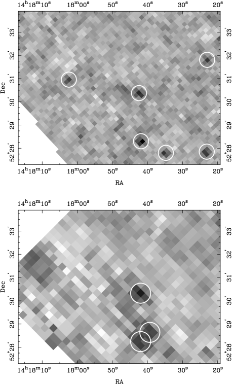
Figure 1: MIPS observations of the CUDSS 14h field at 70$\mu$m (top) and 160$\mu$m (bottom). Sources detected with $\geq 3\sigma$ significance are circled. Blank regions are masked areas of poor or no coverage.

The error images output by the current version of the SSC pipeline are only an estimate of the true error and do not accommodate for the full range of effects exhibited by the MIPS detectors. Also, the MIPS image data are covariant as a result of pixel interpolation and rebinning carried out during pipeline construction of the mosaics. This covariance must be quantified and incorporated into the stacking analysis that follows. For these reasons, we generated our own error data.

To obtain variance images, we made the assumption that the error in the flux of a given pixel is inversely proportional to the square root of the number of times the pixel has been scanned. Of course, pixels containing bright sources will have an additional contribution from Poisson noise, but since our data have very few bright sources and since we investigate their effect on the stacking by removing them, this is not a concern. The variance images are then the inverse of the coverage maps scaled to have a standard deviation of unity. Indeed, we recover a perfect Gaussian distribution of pixel signal to noise (apart from a few outliers due to bright sources) when the variance is calculated in this manner.

Pixel covariances were derived directly from the image data. We calculated the average covariance for all pixel pair configurations (up to a separation such that the covariance was negligible) over image areas away from bright sources. Avoiding areas with bright sources helps minimise the overestimation caused by the instrumental PSF. Nevertheless, as we discuss in Section 3, the covariance is still overestimated by a small amount, meaning that our quoted significances are conservative.

3 Analysis

Rather than follow the procedure of stacking small sections of the image centred on the source positions (see, for e.g., Dole et al., 2006), we opt for the method used in our earlier work (Dye et al., 2006) whereby flux is measured directly from the image at each source position. The catalogue of sources is offset by varying amounts on a 2D regular grid and the flux summed over all sources at each offset. The result is an ‘offset map’ that gives an indication of how well aligned the sources are with respect to the image and the significance of the stacked flux (see Figure 2). As we showed in Dye et al. (2006), if the sources are properly aligned with the image, then the correct stacked flux is that at the origin of the offset map, not necessarily at the peak which may be slightly offset from the origin.

The data stacked in Dye et al. (2006) were SCUBA maps with each pixel value representing the total flux a point source would have if located within that pixel. The stacking therefore simply took the sum of all map pixel values at the source positions. In the current work, the MIPS data output by the pipeline adhere to the usual optical convention whereby a pixel holds the flux received solely by that pixel. A source’s total flux is therefore the sum of flux in all pixels belonging to the source. To convert the MIPS data into the convention used by the SCUBA data in preparation for stacking, we convolved the images with a circular top-hat, then multiplied them by the aperture correction corresponding to the top-hat radius. The convolution was carried out at the original pixel scale of each image, so to prevent aliasing effects, pixels around the top-hat circumference were weighted by their interior fractional area.

Our choice of a circular top-hat instead of the more conventional instrument PSF was based on the fact that the MIPS PSF varies between sources and between images. We created simulated MIPS images of a point source, varying the asymmetry and size of the image PSF compared to the fiducial model PSF in each case. We found that the error in the total source flux measured by convolving with the fiducial PSF rises more quickly with increasing PSF asymmetry and size than measured by convolving with a circular top-hat having an aperture correction matched to the fiducial PSF. The MIPS data handbook recommends that the PSF should be determined directly from bright sources in the image, but since our image has no sufficiently bright sources, this was not possible.

With this in mind, we chose top-hat radii of $r=18^{\prime\prime}$ and $r=40^{\prime\prime}$ for the 70 and 160$\mu$m images respectively. Instead of using the corresponding aperture corrections from the MIPS data handbook, we computed our own to ensure consistency with our top-hat convolution. For each wavelength, we took the in-orbit PSF, binned it to the relevant image pixel scale, then computed its product with the edge-weighted top-hat to give the fraction of flux contained within the top-hat and hence the aperture correction. For the 70$\mu$m data, we measured an aperture correction of 1.63 for the $r=18^{\prime\prime}$ top-hat and for the 160$\mu$m data with the $r=40^{\prime\prime}$ top-hat, an aperture correction of 1.53. These are $\sim 5\%$ smaller than the low temperature aperture corrections given in the MIPS handbook.

In this paper, we quote an average stacked flux per source, $\overline{f}=\Sigma_{i=1}^{N}f_{i}/N$ and an average inverse variance weighted flux per source, $\overline{f}_{w}=\Sigma_{i}(f_{i}\sigma_{i}^{-2})/\Sigma_{i}\sigma_{i}^{-2}$. Here, $f_{i}$ and $\sigma_{i}$ are respectively the flux and $1\sigma$ uncertainty on the top-hat convolved image pixel populated by source $i$. Comparison of the average flux with the weighted average flux gives an indication of whether the stacked signal is dominated by a minority of high significance sources. Simple error propagation shows that $\sigma_{i}$ is given by

$$\sigma_{i}^{2}=\sum_{j,k}t_{j-i}t_{k-i}c_{jk}$$ (1)

where $t_{i}$ is the value of the top-hat function in pixel $i$ and $c_{jk}$ is the covariance in the original, unconvolved image between pixels $j$ and $k$. As explained in Section 2.2, the variances, i.e., diagonal terms of $c_{jk}$, come from the variance image, computed for each image pixel from the coverage map. However, the off-diagonal terms are the covariances averaged over the whole image, so that any pixel pair $jk$ with the same separation vector are assigned the same covariance.

To verify our treatment of errors, for each of the 70 and 160$\mu$m data, we fitted a Gaussian to the distribution of flux significance in the original unconvolved images, and to the distribution of the significance, $f_{i}/\sigma_{i}$, for the convolved images. In the latter case, we first included, then omitted the off-diagonal elements in the covariance matrix. With the original 70 and 160$\mu$m images, the Gaussian fit had unit standard deviation as expected. With the convolved images and the off-diagonal covariance terms included, the standard deviation for the 70$\mu$m image was approximately 0.95 and for the 160$\mu$m image, 0.90. However, including only the variance terms gave a standard deviation of 1.79 for the 70$\mu$m data and 2.78 for the 160$\mu$m data. This test confirms two facts: 1) If covariance is not allowed for, the stacked flux error is underestimated by $\sim 45\%$ at 70$\mu$m and $\sim 65\%$ at 160$\mu$m. 2) Our measurement of covariance is slightly overestimated, presumably due to the MIPS PSF, giving rise to a conservative 5-10% underestimate of the stacked flux significance.

Finally, source confusion due to the large 70 and 160$\mu$m MIPS PSF must also be accounted for in the stacking. With the nodded and chopped SCUBA data of Dye et al. (2006), this could be neglected because the beam and hence the map in these data had an average of zero. With the MIPS data, this is not so. The average stacked flux per source must therefore be corrected by subtracting off the average of the convolved image then dividing the result by the factor $(1-B_{e}/A)$, where $B_{e}$ is the effective area of the PSF of the convolved image and $A$ is the image area (see Appendix A).

4 Results

To investigate the contribution from bright, directly detectable sources in the MIPS images to the average stacked flux, we carried out two stacks per image, one leaving the image unaltered and a second with all $\geq 3\sigma$ sources removed. At 70$\mu$m, there are six $\geq 3\sigma$ sources, whereas at 160$\mu$m, there are three (see Figure 1). Sources were removed by subtracting the in-orbit PSFs from the images at the position of each source, scaled to match the integrated source brightness.

4.1 Stacking the full SCUBA, 24$\mu$m and 8$\mu$m catalogues

The results of stacking all (i.e., not selected by redshift) SCUBA, 24$\mu$m and 8$\mu$m sources onto the MIPS data are given in Table 1. Offset maps showing the average weighted flux per source for each combination of MIPS image and source list are also plotted in Figure 2. Errors in both the table and the maps include the uncertainty of the calibration on the 70 and 160$\mu$m data.

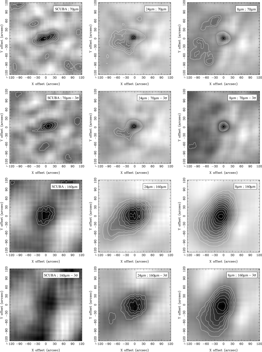
Figure 2: Offset maps of average weighted stacked flux per source ($\overline{f}_{w}$) for all combinations of MIPS image and sources stacked. Columns from left to right correspond to SCUBA sources, 24$\mu$m sources and 8$\mu$m sources. First and second rows correspond to 70$\mu$m MIPS data including then excluding $\geq 3\sigma$ sources respectively. Similarly, third and fourth rows correspond to 160$\mu$m MIPS data including then excluding the $\geq 3\sigma$ sources. Contours start at $2\sigma$ significance and increase by $0.5\sigma$ intervals. Average fluxes for each case are given in Table 1. Significances account for the MIPS 70 and 160$\mu$m calibration uncertainty. The number of sources stacked for each of the different combinations are: 20 (SCUBA/70), 22 (SCUBA/160), 177 (24/70), 171 (24/160), 801 (8/70) and 773 (8/160).

MIPS Data	850$\mu$m SCUBA Sources	24$\mu$m Sources	8$\mu$m Sources
70$\mu$m	3.63$\pm$0.77 (3.45$\pm$0.80)	2.04$\pm$0.25 (2.10$\pm$0.25)	0.95$\pm$0.12 (0.83$\pm$0.12)
70$\mu$m - 3$\sigma$ sources	2.51$\pm$0.77 (2.58$\pm$0.78)	1.64$\pm$0.24 (1.65$\pm$0.24)	0.64$\pm$0.12 (0.57$\pm$0.12)
160$\mu$m	19.9$\pm$6.4 (16.9$\pm$6.6)	15.0$\pm$2.4 (14.9$\pm$2.4)	8.5$\pm$1.1 (8.2$\pm$1.1)
160$\mu$m - 3$\sigma$ sources	9.5$\pm$6.6 (8.1$\pm$6.7)	8.8$\pm$2.2 (8.6$\pm$2.2)	5.6$\pm$1.0 (5.4$\pm$1.0)

Table 1: Average weighted flux per stacked source ($\overline{f}_{w}$) in mJy for the MIPS 70 and 160$\mu$m images, including and having subtracted $\geq 3\sigma$ sources. These correspond to the flux at $(0,0)$ in the offset maps shown in Figure 2. Quantities in parentheses are the average unweighted fluxes $\overline{f}$. All errors include the MIPS 70 and 160$\mu$m calibration uncertainty.

Apart from a single case, i.e., the instance in which SCUBA sources were stacked onto the 160$\mu$m MIPS image with $\geq 3\sigma$ sources removed, every stacking combination results in a significant detection of far-IR flux. All peaks in the offset maps are well aligned with the origin. This indicates that all data are properly aligned, as we expected since all Spitzer data are tied to 2MASS (Two Micron All Sky Survey; Cutri et al., 2003) and we showed in Dye et al. (2006) that the SCUBA data are well aligned with the Spitzer data. The more extended nature of the peaks in the 160$\mu$m offset maps is a reflection of the broader PSF at this wavelength (40″FWHM, compared to 18″at 70$\mu$m).

The differences between the $3\sigma$ source-subtracted and unmodified stacks show that at both 70 and 160$\mu$m, the $\geq 3\sigma$ sources account for approximately 50% of the average flux per source, across all three source populations. In every case, the average flux per SCUBA source is highest, followed by the average flux per 24$\mu$m source then per 8$\mu$m source. This is not surprising; the 70 and 160$\mu$m data are sensitive to the same dusty population of sources as SCUBA, whereas the 8$\mu$m data are also sensitive to distant older stellar populations. Also, the fact that there are more objects in the 24 and 8$\mu$m catalogues brings the average flux down because on average, these sources will sample more image noise than areas of significant 70 and 160$\mu$m emission.

Dole et al. (2006) stack 24$\mu$m sources with fluxes $\geq 60\mu$Jy onto MIPS data to measure a flux of $0.138\pm 0.024$ MJy/sr at 70$\mu$m and $0.571\pm 0.123$ MJy/sr at 160$\mu$m. Using our MIPS data with all $\geq 3\sigma$ sources removed, we find a lower contribution of 0.070$\pm$0.010 MJy/sr at 70$\mu$m and 0.36$\pm$0.09 MJy/sr at 160$\mu$m. However, a contribution of 0.103$\pm$0.019 MJy/sr at 70$\mu$m and 0.87$\pm$0.16 MJy/sr at 160$\mu$m is made by the $8\mu$m sources, again having removed the $\geq 3\sigma$ sources. Within the errors and including the fact that our data are more prone to cosmic variance (see below) being $\sim 80$ times smaller in areal coverage, our results are consistent with those of Dole et al. (2006).

To estimate of the effects of cosmic variance on our results, we divided the data into two approximately equal areas and then repeated the stacking with the halved data. This was performed twice, firstly splitting by the median source RA of each source catalogue, then by the median Declination. The $1\sigma$ variation in the spread of the resulting stacked 70$\mu$m flux was found to be $\sim 30\%$ and the variation in the 160$\mu$m flux, $\sim 20\%$. Since this is an estimate of the variance between fields half the size, the variance between fields of the full size, discounting clustering effects, will be a factor of $\sqrt{2}$ smaller, i.e., $\sim 20\%$ at 70$\mu$m and $\sim 15\%$ at 160$\mu$m. As this serves merely as an order-of-magnitude estimate of the cosmic variance, we do not include it in any of the errors quoted in this paper.

4.1.1 Contribution of sources to the CIB

The total contribution of the three different source populations to the CIB is given in Table 2. By extrapolation, Chapman et al. (2005) estimated an upper limit on the contribution of $>1$mJy SCUBA sources detected at 850$\mu$m to the CIB emission at 160$\mu$m of $\mathbin{\lower 3.0pt\hbox{$\hbox to0.0pt{\raise 5.0pt\hbox{$\char 60\relax$}\hss}\mathchar 29208\relax$}}0.04$ MJy/sr. Despite our CUDSS sources having a brighter sensitivity level of 3.5mJy, we measure a higher contribution at 160$\mu$m of 0.125$\pm$0.040 MJy/sr, without removing any bright MIPS sources, or 0.060$\pm$0.042 MJy/sr having removed all $\geq 3\sigma$ sources. Although these measurements have large uncertainties, they suggest the possibility of a somewhat larger SCUBA source contribution to the 200$\mu$m CIB peak than previously thought.

Table 2 shows that at both 70 and 160$\mu$m, the SCUBA sources make the lowest total contribution, followed by the 24$\mu$m sources and then the 8$\mu$m sources with the highest contribution. This is an important result; sources on the shorter wavelength side of the peak in the CIB resolve more of the CIB at 70 and 160$\mu$m, and therefore most likely at the 200$\mu$m peak itself, than the SCUBA sources on the longer wavelength side. This is almost entirely due to the differing sensitivities of the source populations used for stacking. In terms of the efficiency of resolving the bulk of the CIB emission, the 8 and 24$\mu$m source population are more favourable than the SCUBA sources. This is not surprising because SCUBA surveys typically find 0.4 sources per arcmin² for each hour of observation whereas Spitzer surveys find $\sim 130$ 8$\mu$m sources per arcmin² for each hour of observation. Of course, in the context of the present study, SCUBA’s time would be more efficiently used by computing the cross correlation of the 850$\mu$m maps with the Spitzer images, rather than merely stacking at the positions of significant SCUBA sources. We will carry out this cross correlation in future work.

MIPS Data	SCUBA	24$\mu$m	8$\mu$m
70$\mu$m	0.021$\pm$0.005	0.087$\pm$0.011	0.152$\pm$0.019
70$\mu$m - 3$\sigma$	0.014$\pm$0.004	0.070$\pm$0.010	0.103$\pm$0.019
160$\mu$m	0.125$\pm$0.040	0.62$\pm$0.10	1.31$\pm$0.17
160$\mu$m - 3$\sigma$	0.060$\pm$0.042	0.36$\pm$0.09	0.87$\pm$0.16

Table 2: Contribution of sources to the CIB at 70 and 160$\mu$m in units of MJy/sr, computed from the average weighted flux per source given in Table 1. The coverage for each source catalogue is as follows: 41 arcmin² for 850$\mu$m SCUBA sources, 49 arcmin² for the 24$\mu$m sources and 59 arcmin² for the 8$\mu$m sources.

Expressing the absolute contributions in Table 2 as a fraction of the CIB is somewhat difficult due to the uncertainty in the background flux at 70 and 160$\mu$m (primarily because of differing estimates of foreground contamination). In fact, there are no direct measurements at these specific wavelengths. The most reliable measurements close to 160$\mu$m are those at 140$\mu$m made by the Diffuse Infrared Background Experiment (DIRBE) on board the Cosmic Background Explorer. Depending on the calibration used, the DIRBE results give a flux of either $1.17\pm 0.32$ MJy/sr or 0.70 MJy/sr at 140$\mu$m (Hauser et al., 1998), although as noted by Dole et al. (2006), the zodiacal cloud colours of Kelsall et al. (1998) imply that a further 0.14 MJy/sr should be subtracted from these numbers. Taking the average of both calibrations and subtracting 0.14 MJy/sr gives a flux of 0.80 MJy/sr. This can be extrapolated to give an approximation of the flux at 160$\mu$m of 0.99 MJy/sr using the SED fit to the CIB by Fixsen et al. (1998). DIRBE also provided estimates of the CIB at 60$\mu$m which are a useful constraint on our measurement of the background at 70$\mu$m with MIPS. Finkbeiner, Davis & Schlegel (2000) placed an upper limit on the CIB at 60$\mu$m of $0.56\pm 0.14$ MJy/sr. More recently, this limit was reduced to 0.3 MJy/sr by Dwek & Krennrich (2005).

In terms of lower limits on the CIB at these wavelengths, stacking analyses are currently the most stringent. By effectively extrapolating their 24$\mu$m number counts, Dole et al. (2006) currently provide the highest lower limits on the CIB of 0.17$\pm$0.03 MJy/sr at 70$\mu$m and 0.71$\pm$0.09 MJy/sr at 160$\mu$m. Using these and taking the DIRBE measurements quoted above as upper limits, we can estimate the range in fractional contribution that our strongest contributors, the 8$\mu$m sources, make to the CIB. The upper limit to the CIB at 60$\mu$m imposed by Dwek & Krennrich (2005) and the extrapolated lower limit of Dole et al. (2006) at 70$\mu$m indicates that our 8$\mu$m sources resolve $\sim 35-75$% of the background at 70$\mu$m. Similarly, taking the DIRBE extrapolation to 160$\mu$m as an upper limit and the extrapolated lower limit of Dole et al. (2006) at 160$\mu$m implies that $\sim 90-100$% of the 160$\mu$m background is resolved by the 8$\mu$m sources.

To what extent do the additional 8$\mu$m sources not detected in the 24$\mu$m data emit at far-IR wavelengths? This can be very crudely estimated by calculating the number of 8$\mu$m sources that would be required to give the same measured CIB contribution but assuming each source has a constant flux equal to the corresponding average 24$\mu$m source flux. Here, the assumption is made that all the 24$\mu$m sources (95% of which are detected at 8$\mu$m) contribute to the far-IR flux. This simple calculation, shows that $\sim 20\%$ and $\sim 50\%$ of the additional 8$\mu$m sources at 70 and 160$\mu$m respectively would have to contribute in that case. This is a conservative estimate because in reality, the average far-IR flux of the additional 8$\mu$m sources will be lower than the average flux of the 24$\mu$m sources due to the increased sensitivity of IRAC at 8$\mu$m.

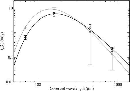
Figure 3: SED fits to the average 8$\mu$m (black line, open circles) and 24$\mu$m (grey line, filled circles) source fluxes for the median source redshift of $z=1$. Data points at 70 and 160$\mu$m are taken from the present study and those at 450 and 850$\mu$m from Dye et al. (2006). Both SEDs show that the average 8 and 24$\mu$m sources detected by Spitzer in this dataset are borderline ULIRGs.

4.1.2 Average 8 & 24$\mu$m source SEDs

In Dye et al. (2006) we measured the average 450 and 850$\mu$m flux per 24 and 8$\mu$m source. Combining these measurements with the average 70 and 160$\mu$m flux per 24 and 8$\mu$m source determined in the present work gives four data points each to which we can fit average SEDs. Figure 3 shows the results of fitting the grey-body function $A\nu^{\beta}{\rm B}(\nu,{\rm T})$ to these average fluxes, where $A$ is a normalisation constant and B is the Planck function. In the fit, the parameters $A$, $\beta$ and T were allowed to vary and we redshifted the function to the median redshift of our sample, $z=1.0$.

For the 24$\mu$m sources, the best fit is achieved with $\beta=2.05^{+1.03}_{-0.59}$ and T = $39.7^{+5.7}_{-5.4}$K and for the 8$\mu$m sources with $\beta=1.54^{+0.27}_{-0.28}$ and T = $38.8^{+3.2}_{-2.7}$K ($1\sigma$ errors quoted). The dependence of these fitted parameters on the median redshift is such that a change in redshift $\Delta z$ produces a change in T given by $\Delta{\rm T}\simeq 19\Delta z$ for both 24 and 8$\mu$m sources, while $\beta$ has absolutely no dependence. The temperature of our average sources is consistent with temperatures of submm galaxies found in the local universe, e.g., Dunne & Eales (2001) who measure T=$(36\pm 5)$K. Whether there is consistency with submm sources in the high redshift Universe is less clear. The sample of 73 SCUBA sources with a median redshift of 2.3 of Chapman et al. (2005) has a median temperature of T${}_{\rm med}\simeq(36\pm 7)$K, consistent with our values. However, the sample of 10 SCUBA sources with a median redshift of 1.7 of Pope et al. (2006) has a lower median temperature of T${}_{\rm med}\simeq 30$K. If a discrepancy exists, then it could be explained, at least in part, by the selection effect noted by Chapman et al. (2005); surveys like that of Pope et al. (2006) requiring a submm and radio detection are biased toward colder sources.

The normalisation of both SEDs confirms that the average 24 and 8$\mu$m source detected by Spitzer in the current sample is a borderline ultra-luminous infrared galaxy (ULIRG). To demonstrate this, we use the definition of Clements, Saunders & McMahon (1999) that stipulates a ULIRG must have a luminosity of at least $2.5\times 10^{11}$L_⊙ measured at 60$\mu$m by the Infra-Red Astronomical Satellite (IRAS). The rest-frame 60$\mu$m flux computed from our best fit SEDs is $2.3\times 10^{11}$L_⊙ for the average 24$\mu$m source and $1.2\times 10^{11}$L_⊙ for the average 8$\mu$m source, in good agreement with Dye et al. (2006).

An interesting question is how do our average 24 and 8$\mu$m sources compare to the average SCUBA source detected by other studies? Pope et al. (2006) define the quantity L_IR as the integral of flux in the wavelength range 8 - 1000$\mu$m. Their sample of 10 SCUBA sources has a median L_IR of $6.0\times 10^{12}$L_⊙. Similarly, the median value of L_IR for the sample of 73 SCUBA sources of Chapman et al. (2005) is $8\times 10^{12}$L_⊙. In comparison, our average 24$\mu$m SED gives L${}_{\rm IR}=5.8\times 10^{11}$L_⊙ and our average 8$\mu$m SED L${}_{\rm IR}=3.5\times 10^{11}$L_⊙. The average 24 and 8$\mu$m source in our sample is therefore $\sim 10$ times fainter than the average SCUBA source detected by the previous two studies.

4.2 Stacking the 24 and 8$\mu$m sources by redshift

In this section, we consider the contribution from the 24 and 8$\mu$m sources to the CIB at 70 and 160$\mu$m as a function of redshift. Using the photometric redshifts already determined in Dye et al. (2006), we divided the sources equally into redshift bins of varying width. The source redshifts extend up to $z\simeq 4$ (see Figure 3 of Dye et al., 2006). Bins were chosen to be large compared to the average redshift uncertainty but small enough to give reasonable resolution, hence the 24$\mu$m sources were divided into 5 redshift bins and the 8$\mu$m sources into 6. Approximately 10% of sources with undetermined redshifts (due to their sparse optical photometry) were omitted from the analysis of this section. This therefore gives $\sim 30$ objects per 24$\mu$m bin and $\sim 120$ objects per $8\mu$m bin.

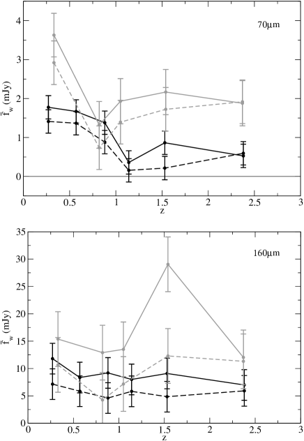
Figure 4: Variation of average weighted 70$\mu$m flux (top) and 160$\mu$m flux (bottom) of Spitzer 24 and 8$\mu$m objects binned by redshift. The median redshift in each bin is plotted. Redshifts extend up to $z\simeq 4$ (see Dye et al., 2006) and are divided equally between bins. In both plots, the continuous grey and black lines correspond to the 24 and 8$\mu$m sources respectively, stacked onto the MIPS images without any sources removed. The dashed lines show the average weighted flux having removed the $\geq 3\sigma$ sources from the MIPS images.

Figure 4 shows how the weighted average 70 and 160$\mu$m flux per source varies with redshift. The plots show this variation both having removed the $\geq 3\sigma$ sources in the MIPS images and with them left in place. At 70$\mu$m, the effect of removing the 3$\sigma$ sources has less effect than at 160$\mu$m. Also, at 70$\mu$m, the flux is dominated by 8$\mu$m sources lying at lower redshifts. Dividing the 8$\mu$m sources into two populations segregated by the median redshift, $z=1.0$, the low redshift population accounts for $(79\pm 10)\%$ of the total 70$\mu$m emission (having removed the $\geq 3\sigma$ sources) from the 8$\mu$m sources. In comparison, the 70$\mu$m emission per 24$\mu$m source is more evenly spread in redshift, the low redshift population accounting for $(51\pm 10)\%$. At 160$\mu$m, the low redshift 8$\mu$m sources contribute $(52\pm 14)\%$ of their total and the 24$\mu$m sources contribute $(42\pm 15)\%$, having removed all $\geq 3\sigma$ 160$\mu$m sources.

The differences between the 70 and 160$\mu$m plots in Figure 4 are very well explained by a single average source SED consistent with the fitted average SEDs derived in section 4.1.2. To demonstrate this, we took an SED from Dale & Helou (2002) corresponding to a dust temperature of T=40K to match our average SEDs. Since this SED extends into the optical and models typical mid-IR spectral features due to dust, a realistic prediction of the 70 and 160$\mu$m flux of a source given its redshift and 8 or 24$\mu$m flux can be made. In this way, using our 8 and 24$\mu$m source catalogues, we computed a prediction of the variation of 70 and 160$\mu$m flux with redshift.

The results of this analysis are shown in Figure 5. There is good agreement between our measured variation and the predicted variation. We reproduce the total flux (summed over all sources) within the errors and also the observed trends. Most notably, we reproduce the decline in the 70$\mu$m emission from the 8$\mu$m sources within $0<z<1$ as the peak of the SED is redshifted out of the 70$\mu$m band. This explains why the majority of 70$\mu$m emission is observed from the 8$\mu$m sources lying at $z\leq 1$. The prediction degrades quickly if a cooler or warmer SED is used; with a 35K or 45K SED, the total predicted flux is inconsistent with the total measured. The fact that a single SED can be used to fit the observed flux over such a wide range of redshifts implies that only a small amount of source evolution must have occured during that time.

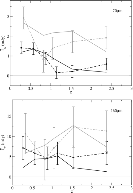
Figure 5: Comparison of the measured (dashed lines) and predicted (continuous lines) MIPS 70 and 160$\mu$m flux from the 8$\mu$m (black) and 24$\mu$m (grey) sources using a T=40K SED taken from Dale & Helou (2002). The measured data are the stacked fluxes in Figure 4 with $\geq 3\sigma$ sources removed.

To assess the effects of cosmic variance on the results of this section, we repeated the previous exercise of dividing the data into halves and re-stacking. We found that the major trends are robust, i.e., the decline in 70$\mu$m flux from the 8$\mu$m sources over the interval $0<z<1$ and that the other combinations remain consistent with little or no variation with redshift. However, the large spike in 160$\mu$m flux seen from the 24$\mu$m sources at $z\sim 1.5$ (without having removed the $\geq 3\sigma$ sources) is not robust and therefore presumably an effect of cosmic variance.

5 Summary and Discussion

In this paper, we have quantified the contribution of flux to the CIB at 70 and 160$\mu$m from SCUBA sources and 24 and 8$\mu$m Spitzer sources in the CUDSS 14hour field. By stacking flux at the position of the different sources, we have found that the SCUBA sources make the highest contribution per source and that the 8$\mu$m sources make the lowest. Conversely, the opposite is true of the total contribution from all sources, leading to the conclusion that the bulk of the CIB is most efficiently resolved by sources detected at wavelengths shorter than the peak of the CIB emission at $\sim 200\mu$m.

Our stacking suggests a somewhat larger contribution from the CUDSS SCUBA sources to the 200$\mu$m CIB peak than previously thought. Chapman et al. (2005) estimated an upper limit on the contribution of $>1$mJy SCUBA sources detected at 850$\mu$m to the CIB emission at 160$\mu$m of $\mathbin{\lower 3.0pt\hbox{$\hbox to0.0pt{\raise 5.0pt\hbox{$\char 60\relax$}\hss}\mathchar 29208\relax$}}0.04$ MJy/sr. Despite our SCUBA sources having a brighter sensitivity level of 3.5mJy, we measure a contribution at 160$\mu$m of 0.125$\pm$0.040 MJy/sr, without removing any bright MIPS sources, or 0.060$\pm$0.042 MJy/sr having removed all $\geq 3\sigma$ sources.

Since measurements of the CIB at 70 and 160$\mu$m are presently very uncertain, the fractional contribution to the CIB made by our sources can only be expressed within a range set by present upper and lower limits. Using the DIRBE estimates as upper limits and the lower limits set by Dole et al. (2006), our strongest contributors, the 8$\mu$m sources, resolve somewhere between $\sim 35-75$% of the background at 70$\mu$m and $\sim 90-100$% at 160$\mu$m.

By combining our results in the present work with our previous stacking of 450 and 850$\mu$m SCUBA flux (Dye et al., 2006), we have established that the 8 and 24$\mu$m sources detected by Spitzer are on average borderline ULIRGs. The average source we detect is $\sim 10$ times fainter than the average SCUBA source detected by Pope et al. (2006) and Chapman et al. (2005) integrating flux over the wavelength range 8 - 1000$\mu$m. Furthermore, the temperature of $\sim 40$K of our average source is consistent with temperatures of submm galaxies found in the local Universe (e.g., Dunne & Eales, 2001) and with the median temperature of $(36\pm 7)$K of SCUBA sources in the high redshift Universe found by Chapman et al. (2005). However, our average source is warmer than the median temperature of T${}_{\rm med}\simeq 30$K of 10 SCUBA sources measured by Pope et al. (2006).

Using photometric redshifts assigned to the 8 and 24$\mu$m sources, we have investigated how the contribution of 70 and 160$\mu$m flux to the CIB varies with redshift. We have found that the 8$\mu$m sources at low redshifts, $z<1$ (accounting for half of them), are the strongest contributors to the CIB at 70$\mu$m, their flux amounting to $\sim 4$ times that of the $z>1$ sources. The 70$\mu$m emission per 24$\mu$m source as well as the 160$\mu$m emission per 8 and 24$\mu$m source is consistent with an even distribution over redshift. This verifies the result of Dole et al. (2006) that the majority of the emission at 70 and 160$\mu$m from 24$\mu$m sources must come from a redshift of $z\sim 1$ where the redshift distribution of these sources peaks. We have shown how this distribution can be reproduced from our observed 8 and 24$\mu$m catalogue of fluxes and redshifts using a single non-evolving source SED with a dust temperature of 40K.

As a concluding remark, this study and similar recent studies (e.g., Serjeant et al., 2004; Knudsen et al., 2005; Dye et al., 2006; Wang, Cowie & Barger, 2006) indicate that the CIB is not predominantly due to a rare population of exceptionally luminous submillimeter sources as hinted at by early SCUBA observations, but that a much more numerous galaxy population of modest average luminosity is responsible instead. However, we have shown here that the SCUBA galaxies probably do make a larger contribution than previously thought, although much larger numbers of SCUBA sources such as those of the SCUBA half degree extragalactic survey (SHADES; Mortier et al., 2005) or those resulting from future SCUBA2 surveys will be required to improve the precision of these measurements.

Appendix A Flux boosting correction

In the following, it is assumed that the MIPS image has been prepared such that the value of any one pixel gives the total flux a point source would have if located within that pixel. Since this preparation inevitably involves convolution of the raw MIPS image with some kind of kernel, the profile of a point source will be the convolution of this kernel with the original image PSF. This resulting profile is referred to as the image ‘beam’ hereafter.

Suppose that $T$ is the total number of sources being stacked onto the MIPS image and that a subset $N$ of these are ‘genuine’ sources. A source is defined as ‘genuine’ if it has associated MIPS emission that makes a non-negligible contribution to the stacked flux. (In practice, one would derive a threshold flux that depends on the number of sources). The actual average flux per source is then simply the summed flux from the genuine sources divided by the total number of sources,

$$\overline{f}_{\rm actual}=\frac{1}{T}\sum_{i}^{N}f_{i}\,\,,$$ (A1)

where $f_{i}$ is the flux in the MIPS image pixel at the position of the genuine source $i$.

However, this quantity is overestimated if one naively adds the flux in the MIPS image at the positions of all $T$ sources for two reasons. Firstly, the $T-N$ sources without associated MIPS emission (the ‘contaminating’ sources) sample flux from the genuine sources since some will happen to lie within genuine source beams. The extra flux sampled on average from a genuine source with flux $f_{i}$ by the contaminating sources is

$$f^{c}_{i}=2\pi n_{c}f_{i}\int rb(r){\rm d}r=n_{c}B_{e}f_{i},$$ (A2)

where $b(r)$ is the radial beam profile scaled to have a peak height of unity, $n_{c}$ is the number density of contaminating sources and $B_{e}$ defines the effective beam area. Secondly, the genuine sources themselves sample emission from neighbouring genuine sources when their beams overlap. Similar to the contaminating sources, the extra flux sampled on average from a genuine source with flux $f_{i}$ by its neighbouring genuine sources is

$$f^{g}_{i}=n^{\prime}_{g}B_{e}f_{i}\,\,,$$ (A3)

where $n^{\prime}_{g}$ is the number density of the neighbouring $N-1$ genuine sources. The average MIPS flux per source that is measured by summing the flux at all $T$ source positions is therefore

$$\overline{f}_{\rm measured} = \frac{1}{T}\sum_{i}^{N}(f_{i}+f^{c}_{i}+f^{g}_{i})=\frac{1+n^{\prime}_{t}B_{e}}{T}\sum_{i}^{N}f_{i}$$ (A4)

$$= (1+n^{\prime}_{t}B_{e})\overline{f}_{\rm actual}\,\,,$$

where $n^{\prime}_{t}=n^{\prime}_{g}+n_{c}$ is the number density of $T-1$ sources. The measured average flux is therefore the actual average flux boosted by a factor of $(1+n^{\prime}_{t}B_{e})$.

If the MIPS data are properly normalised, (so that there is no net positive emission from artifacts, systematic effects, etc.) then the average of the image over its area $A$ is

$$\overline{f}_{\rm image}=\frac{B_{e}}{A}\sum_{i}^{N}f_{i}=\frac{n_{t}B_{e}}{T}\sum_{i}^{N}f_{i}=n_{t}B_{e}\overline{f}_{\rm actual}\,\,,$$ (A5)

having used the fact that the number density of all $T$ sources is $n_{t}=T/A$. Subtracting equation (A5) from equation (A4) and rearranging gives

$$\overline{f}_{\rm actual}=(\overline{f}_{\rm measured}-\overline{f}_{\rm image})(1-B_{e}/A)^{-1}\,\,,$$ (A6)

hence the actual average flux per source can be obtained by subtracting the image average and dividing by the factor $(1-B_{e}/A)$.

In the above, it has been assumed that source positions are a random sampling of a uniform distribution. In reality, the sources will exhibit a degree of clustering. Clustering of the genuine sources causes a positive bias of the average flux compared to the non-clustered assumption, whereas clustering of the contaminating sources on average has no effect.

Acknowledgements

SD is supported by the U.K. Particle Physics and Astronomy Research Council. Part of the research described in this paper was carried out at the Jet Propulsion Laboratory, California Institute of Technology, under a contract with the National Aeronautics and Space Administration. The Spitzer Space Telescope is operated by the Jet Propulsion Laboratory, California Institute of Technology under NASA contract 1407. Support for this work was provided by NASA through contract 1256790 issued by JPL/Caltech. We thank Herve Dole for refereeing this work and providing several helpful suggestions which have enhanced this paper.

References

- Ashby et al. (2006) Ashby, M. L. N., Dye, S., Huang, J.-S., Eales, S., Webb, T. M. A., Barmby, Willner S. P., Rigopoulou D., Egami E., McCracken H. Lilly S., Miyazaki S., Brodwin M., Blaylock M., Cadien J., Fazio G. G., 2006, ApJ, 644, 778
- Chapman et al. (2005) Chapman, S. C., Blain, A. W., Smail, I., Ivison, R. J., 2005, ApJ, 622, 772
- Clements, Saunders & McMahon (1999) Clements, D.L., Saunders, W.J. & McMahon, R.G., 1999, MNRAS, 302, 391
- Cutri et al. (2003) Cutri, R.M., et al. 2003, Explanatory Supplement to the 2MASS Second Incremental Data Release, IPAC
- Dale & Helou (2002) Dale, D. & Helou, G., 2002, ApJ, 576, 159
- Dole et al. (2004) Dole, H. et al, 2004, ApJS, 154, 87
- Dole et al. (2006) Dole, H., Lagache, G., Puget, J.-L., Caputi, K. I., Fernández-Conde, N., Le Floc’h, E., Papovich, C., Pérez-González, P. G., Rieke, G. H., Blaylock, M., 2006, A&A, 451, 417
- Dunne & Eales (2001) Dunne, L., & Eales, S.A., 2001, MNRAS, 327, 697
- Dwek & Krennrich (2005) Dwek, E. & Krennrich, F., 2005, ApJ, 618, 657
- Dye et al. (2006) Dye, S., et al., 2006, ApJ, 644, 769
- Eales et al. (2000) Eales, S., Lilly, S., Webb, T., Dunne, L., Gear, W., Clements, D., Yun, M., 2000, AJ, 120, 2244
- Fazio et al. (2004) Fazio, G.G., et al., 2004, ApJS, 154,10
- Finkbeiner, Davis & Schlegel (2000) Finkbeiner, D. P., Davis, M. & Schlegel, D. J., 2000, ApJ, 544, 81
- Fixsen et al. (1998) Fixsen, D.J., Dwek, E., Mather, J.C., Bennet, C.L., Shafer, R.A., 1998, ApJ, 508, 123
- Gordon et al. (2005) Gordon, K. D., et al., 2005, PASP, 117, 503
- Hauser et al. (1998) Hauser, M. G., et al., 1998, ApJ, 508, 25
- Hauser & Dwek (2001) Hauser, M. G. & Dwek E., 2001, ARA&A, 39, 249
- Knudsen et al. (2005) Knudsen, K. K., van der Werf, P., Franx, M., Förster Schreiber, N. M., van Dokkum, P. G., Illingworth, G. D., Labbé, I., Moorwood, A., Rix, H. -W., Rudnick, G., 2005, ApJ, 632, 9
- Kelsall et al. (1998) Kelsall, T., Weiland, J. L., Franz, B. A., Reach, W. T., Arendt, R. G., Dwek, E., Freudenreich, H. T., Hauser, M. G., Moseley, S. H., Odegard, N. P., Silverberg, R. F., Wright, E. L., 1998, ApJ, 508, 44
- Lagache, Puget & Dole (2005) Lagache, G., Puget, J.-L. & Dole H., 2005, ARAA, 43, 727
- Mortier et al. (2005) Mortier, A. M. J., et al., 2005, MNRAS, 363, 563
- Papovich et al. (2004) Papovich, C., et al., 2004, ApJS, 154, 70
- Peacock et al. (2000) Peacock, J. A., et al., 2000, MNRAS, 351, 535
- Pope et al. (2006) Pope, A., et al., 2006, MNRAS, 370, 1185
- Rieke et al. (2004) Rieke, G., et al., 2004, ApJS, 154, 25
- Serjeant et al. (2004) Serjeant, S. et al., 2004, ApJS, 154, 118
- Wang, Cowie & Barger (2006) Wang, W. -H., Cowie, L. L. & Barger A. J., 2006, ApJ in press, 647, 1 iss., astro-ph/0512347
- Webb et al. (2003) Webb, T. M. A., Lilly, S. J., Clements, D. L., Eales, S., Yun, M., Brodwin, M., Dunne, L., Gear, W. K., 2003, ApJ, 597, 680
- Werner et al. (2004) Werner, M., et al., 2004, ApJS, 154, 1