The signature of local cosmic structures on the ultra-high energy cosmic ray anisotropies

Abstract

Current experiments collecting high statistics in ultra-high energy cosmic rays (UHECRs) are opening a new window on the universe facing the possibility to perform UHECR astronomy. Here we discuss a large scale structure (LSS) model for the UHECR origin for which we evaluate the expected large scale anisotropy in the UHECR arrival distribution. Employing the IRAS PSCz catalogue as tracer of the LSS, we derive the minimum statistics needed to reject or assess the correlation of the UHECRs with the baryonic distribution in the universe, in particular providing a forecast for the Auger experiment.

1 Introduction

At energies above a few $\times 10^{19}\,$eV, which we will refer to as the ultra-high energy (UHE) regime, protons propagating in the Galaxy retain most of their initial direction. Provided that the extragalactic magnetic field (EGMF) is negligible, UHE protons will therefore allow us to probe into the nature and properties of their cosmic sources. However, due to quite steep CR power spectrum, UHECRs are extremely rare (a few particles km^-2 century^-1) and their detection calls for the prolonged use of instruments with huge collecting areas. One further constraint arises from an effect first pointed out by Greisen, Zatsepin and Kuzmin [1, 2] and since then known as GZK effect: at energies $E\;^{>}\!\!\!\!_{\sim}\;5\times 10^{19}$ eV the opacity of the interstellar space to protons drastically increases due to the photo-meson interaction process $p+\gamma_{\rm CMB}\to\pi^{0(+)}+p(n)$ which takes place on cosmic microwave background (CMB) photons. In other words, unless the sources are located within a sphere with radius of ${\cal O}$(100) Mpc, the proton flux at $E\;^{>}\!\!\!\!_{\sim}\;5\times 10^{19}$ eV should be greatly suppressed. However, due to the very limited statistics available in the UHE regime, the experimental detection of the GZK effect has not yet been firmly established.

A detailed knowledge of the UHECR framework is still missing. Only recently, for instance, magnetic fields were included in simulations of large scale structures (LSS) [3, 4]. Qualitatively the simulations agree in finding that EGMFs are mainly localized in galaxy clusters and filaments, while voids should contain only primordial fields. However, the conclusions of Refs. [3] and [4] are quantitatively rather different and it is at present unclear whether deflections in extragalactic magnetic fields will prevent astronomy even with UHE protons or not. Another large source of uncertainty is our ignorance on the chemical composition of UHECRs, mainly due to the need to extrapolate for decades in energy the models of hadronic interactions, though important progress are expected from new high quality data and deconvolution techniques (see e.g. [5]). Future accelerator measurements of hadronic cross sections in higher energy ranges will also ameliorate the situation, but this will take several years at least.

From now on, therefore, we shall work under the assumptions that UHE astronomy is possible, namely: i) proton primaries; ii) EGMF negligibly small; iii) extragalactic astrophysical sources are responsible for UHECRs acceleration. A possibility favoring these hypotheses is that relatively few, powerful nearby sources are responsible for the UHECRs, and the small scale clustering observed by AGASA [6] may be a hint in this direction. However, the above quoted clustering has not yet been confirmed by other experiments with comparable or larger statistics [7, 8], and probably a final answer will come when the Pierre Auger Observatory [9] will have collected enough data. Independently on the observation of small-scale clustering, one could still look for large scale anisotropies in the data, eventually correlating with some known configuration of astrophysical source candidates. In this context, the most natural scenario to be tested is that UHECRs correlate with the luminous matter in the “local” universe. This is particularly expected for candidates like gamma ray bursts (hosted more likely in star formation regions) or colliding galaxies, but it’s also a sufficiently generic hypothesis to deserve an interest of its own.

To this aim we use the IRAS PSCz [10] astronomical catalogue as tracer of Large Scale Structures from which, once that the related selection effects have been taken into account, we derive the related pattern of anisotropies; we then assess the minimum statistics needed to detect the model against the isotropic null hypothesis, in particular providing a forecast for the Auger experiment. Previous attempts to address a similar issue can be found in [11, 12, 13]. Further details of the analysis summarized here can be found in [14].

2 Data and Formalism

2.1 The Catalogue

The IRAS PSCz catalogue [10] contains about 15.000 galaxies and related redshifts with a well understood completeness function down to $z\sim 0.1$ (i.e. down to a redshift which is comparable to the attenuation length introduced by the GZK effect) and a sky coverage of about 84%. The incomplete sky coverage is mainly due to the so called zone of avoidance centered on the galactic plane and caused by galactic extinction and to a few, narrow stripes which were not observed with enough sensitivity by the IRAS satellite (see [10]). These regions are excluded from our analysis with the use of the binary mask available with the PSCz catalogue itself. The mask $\mu$ is defined so that $\mu(\hat{\Omega})=0,1$ if the direction $\hat{\Omega}$ falls respectively inside or outside the blind region.

To correctly employ the catalogue, selection and discreteness systematic effects have to be considered. For the flux selection correction the relevant quantity to be taken into account is the fraction of galaxies actually observed at the various redshifts, a quantity also known as the redshift selection function $\phi(z)$; given $\phi(z)$, the quantity $n(z)/\phi(z)$ represents the experimental distribution corrected for the selection effects, which must be used in the computations. The discreteness effects (or ”shot noise”) are, instead, minimized using the catalogue only until a maximum redshift of $z=0.06$ (corresponding to $180\,h^{-1}{\rm Mpc}$), a fair compromise for which we have still good statistics while keeping the intrinsic statistical fluctuations under control. In any case, due to GZK effect in the energy range $E\geq\,$5$\times 10^{19}\,$eV, the contribution from sources beyond $z\simeq 0.06$ is sub-dominant, thus allowing to assume for the objects beyond $z=0.06$ an effective isotropic source contribution. A detailed discussion of the various catalogue issues can be found in [14] and references therein.

2.2 Analysis

The goal of our analysis is to obtain the underlying probability distribution $f_{\rm LSS}(\hat{\Omega},E)$ to have a UHECR with energy higher than $E$ from the direction $\hat{\Omega}$.

For simplicity here we shall assume that each source of our catalogue has the same probability to emit a UHECR, according to a power law spectrum at the source $E^{-s}$; however, both assumpitions can be easily generalized within the same formalism [13].

A suitable expression for the distribution $f_{\rm LSS}(\hat{\Omega},E)$ can be easily obtained as

$$f_{\rm LSS}(\hat{\Omega},E_{\rm cut})\!\!\!\! \propto \!\!\!\!\sum_{k}\frac{1}{\phi(z_{k})}\frac{\delta(\hat{\Omega}-\hat{\Omega}_{k})}{4\pi d^{2}_{L}(z_{k})}\int_{E_{i}(E_{\rm cut},z_{k})}^{\infty}\!\!\!\!\!\!\!\!\!\!\!\!E^{-s}{\rm d}E$$ (1)

$$= \!\!\!\!\sum_{k}f_{\rm LSS}(k)\ \delta(\hat{\Omega}-\hat{\Omega}_{k}),$$

that can be effectively seen as if at every source $k$ of the catalogue it is assigned a weight $f_{\rm LSS}(k)$ that takes into account geometrical effects through the luminosity distance ($d_{L}^{-2}$), selection effects ($\phi^{-1}$), and physics of energy losses through the integral in d$E$; in this “GZK integral” the upper limit of integration is taken to be infinite, though the result is practically independent on the upper cut used provided it is much larger than 10²⁰ eV; the energy losses are taken into account through the code described in [14] and parameterized in the function $E_{i}(E_{f},z)$, the “initial energy function” giving the energy $E_{i}$ of particle that should be injected at a redshift $z$ to reach the Earth with an energy $E_{f}$.

We choose $E_{\rm cut}=5\times 10^{19}\,$eV that results in a fair compromise between the intensity of the anisotropies (that increases with energy) and the achievable statistics; for this $E_{\rm cut}$ the isotropic contribution to the flux is sub-dominant; however we can take it exactly into account and the weight of the isotropic part is given by $w_{\rm iso}\propto\int_{z_{\rm GZK}}^{\infty}{\rm d}z\,p(z,E_{\rm cut})$ .

Finally, to graphically represent the result, the spike-like map of Eq. (1) is effectively smoothed through a gaussian filter with beamwidth $\sigma=3^{\circ}$.

Given the extremely poor statistics available in UHECR astrophysics, we limit ourselves to address the basic issue of determining the minimum number of events needed to significatively reject “the null hypothesis”. To this purpose, it is well known that a $\chi^{2}$-test is an extremely good estimator and has no ambiguity due to the 2-dimensional nature of the problem respect to the K-S test or the Smirnov-Cramer-von Mises test. A criterion guiding in the choice of the bin size is the following: with $N$ UHECRs events available and $M$ bins, one would expect ${\cal O}(N/M)$ events per bin; to allow a reliable application of the $\chi^{2}$-test, one has to impose $N/M\geq 10$. Each cell should then cover at least a solid angle of $\Delta_{M}\sim 10\times\Delta_{\rm tot}/N$, $\Delta_{\rm tot}$ being the solid angle accessible to the experiment. For $\Delta_{\rm tot}\sim 2\pi$ (50% of full sky coverage), one estimates a square window of side $454^{\circ}/\sqrt{N}$, i.e. $45^{\circ}$ for 100 events, $14^{\circ}$ for 1000 events. Since the former number is of the order of present world statistics, and the latter is the achievement expected by Auger in a few years of operations, a binning in windows of size $15^{\circ}$ represents quite a reasonable choice for our forecast. This choice is also suggested by the typical size of the observable structures, as can be seen in the next section. Notice that the GMF, that induces at these energies typical deflections of about $4^{\circ}$ [15], can be safely neglected for this kind of analysis. The same remark holds for the angular resolution of the experiment.

Moreover, for a specific experimental set-up one must include the proper exposure $\omega_{\rm exp}$, that has to be convolved with the previously found $f_{\rm LSS}$. We properly parameterize and take into account the Auger exposure $\omega_{\rm exp}(\delta)$ as function of declination $\delta$ [14, 16]: contour plots in galactic coordinates are shown in Fig. 1.

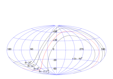
Figure 1: Galactic coordinate reference frame and contours enclosing 68%, 95% and 99% of the Auger exposure function, with the corresponding declinations. The celestial equator ($\delta=0^{\circ}$) and south pole ($\delta=0,-90^{\circ}$) are also shown.

For a given experiment and catalogue, the null hypothesis we want to test is that the events observed are sampled—apart from a trivial geometrical factor—according to the distribution $f_{\rm LSS}\,\omega_{\rm exp}\,\mu$. Since we are performing a forecast analysis, we will consider test realizations of $N$ events sampled according to a random distribution on the (accessible) sphere, i.e. according to $\omega_{\rm exp}\,\mu$, and determine the confidence level (C.L.) with which the hypothesis is rejected as a function of $N$. For each realization of $N$ events we calculate the two functions

$${\cal X}_{\rm iso}^{2}(N)=\frac{1}{M-1}\sum_{i=1}^{M}\frac{(o_{i}-\epsilon_{i}[f_{\rm iso}])^{2}}{\epsilon_{i}[f_{\rm iso}]},$$ (2)

$${\cal X}_{\rm LSS}^{2}(N)=\frac{1}{M-1}\sum_{i=1}^{M}\frac{(o_{i}-\epsilon_{i}[f_{\rm LSS}])^{2}}{\epsilon_{i}[f_{\rm LSS}]},$$ (3)

where $o_{i}$ is the number of “random” counts in the $i$-th bin $\Omega_{i}$, and $\epsilon_{i}[f_{\rm LSS}]$ and $\epsilon_{i}[f_{\rm iso}]$ are the theoretically expected number of events in $\Omega_{i}$ respectively for the LSS and isotropic distribution. The mock data set is then sampled ${\cal N}$ times in order to establish empirically the distributions of ${\cal X}_{\rm LSS}^{2}$ and ${\cal X}_{\rm iso}^{2}$, and the resulting distribution is studied as function of $N$ (plus eventually $s,E_{\rm cut}$, etc.).

3 Results

In Fig. 2 we plot the smoothed maps in galactic coordinates of the expected integrated flux of UHECRs above the energy threshold $E_{\rm cut}=3,5,7,9\times 10^{19}\,$eV and for slope parameter $s=2.0$; the isotropic part has been taken into account and the ratio of the isotropic to anisotropic part $w_{\rm iso}/\sum_{k}f_{\rm LSS}(k)$ is respectively $83\%,3.6\%,\ll 1\%,\ll 1\%$.

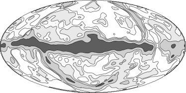
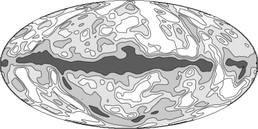
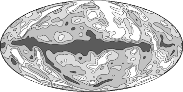
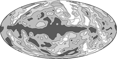
Figure 2: Equal area Hammer-Aitoff projections of the smoothed UHECRs arrival directions distribution (Eq. (1)) in galactic coordinates obtained for fixed $s=2.0$ and, from the upper to the lower panel, for $E_{\rm cut}=3,5,7,9\times 10^{19}$ eV. The smoothing angle is $\sigma=3^{\circ}$. The contours enclose 95%, 68%, 38%, 20% of the corresponding distribution. The dark central band corresponds to the avoidance zone of the galactic plane.

Only for $E_{\rm cut}=3\times 10^{19}\,$eV the isotropic background constitutes then a relevant fraction, since the GZK suppression of far sources is not yet present. For the case of interest $E_{\rm cut}=5\times 10^{19}\,$eV the contribution of $w_{\rm iso}$ is almost negligible, while it practically disappears for $E_{\rm cut}\raise 1.29167pt\hbox{$\;>$\kern-7.5pt\raise-4.73611pt\hbox{$\sim\;$}}7\times 10^{19}\,$eV. Varying the slope for $s=1.5,2.0,2.5,3.0$ while keeping $E_{\rm cut}=5\times 10^{19}\,$eV fixed produces respectively the relative weights $8.0\%,3.6\%,1.8\%,0.9\%$, so that only for very hard spectra $w_{\rm iso}$ would play a non-negligible role.

Due to the GZK-effect, as it was expected, the nearest structures are also the most prominent features in the maps. The most relevant structure present in every slide is the Local Supercluster. It extends along $l\simeq 140^{\circ}$ and $l\simeq 300^{\circ}$ and includes the Virgo cluster at $l=284^{\circ},b=+75^{\circ}$ and the Ursa Major cloud at $l=145^{\circ},b=+65^{\circ}$, both located at $z\simeq 0.01$. The lack of structures at latitudes from $l\simeq 0^{\circ}$ to $l\simeq 120^{\circ}$ corresponds to the Local Void. At higher redshifts the main contributions come from the Perseus-Pisces supercluster ($l=160^{\circ},b=-20^{\circ}$) and the Pavo-Indus supercluster ($l=340^{\circ},b=-40^{\circ}$), both at $z\sim 0.02$, and the very massive Shapley Concentration ($l=250^{\circ},b=+20^{\circ}$) at $z\sim 0.05$. For a more detailed list of features in the map, see the key in Fig. 3.

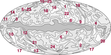
Figure 3: Detailed key of the structures visible in the UHECR maps; arbitrary contour levels. Labels correspond to: (1) Southern extension of Virgo and Local Supercluster; (2)Fornax-Eridani Cluster; (3) Cassiopea Cluster; (4) Puppis Cluster; (5) Ursa Major Cloud; (6-7) Pavo-Indus and ”Great Attractor” region; (8) Centaurus Super-Cluster; (9) Hydra Super-Cluster; (10) Perseus Super-Cluster; (11) Abell 569; (12) Pegasus Cluster; (13-17) Pisces Cluster; (14) Abell 634; (15) Coma Cluster; (16-18) Hercules Supercluster; (19) Leo Supercluster; (20) Columba Cluster; (21) Cetus Cluster; (22) Shapley Concentration; (23) Ursa Major Supercluster; (24) Sculptor Supercluster; (25) Bootes Supercluster.

The $E_{\rm cut}$-dependence is clearly evident in the maps: as expected, increasing $E_{\rm cut}$ results in a map that closely reflects the very local universe (up to $z\sim 0.03-0.04$) and its large anisotropy; conversely, for $E_{\rm cut}\simeq 3,4\times 10^{19}\,$eV, the resulting flux is quite isotropic and the structures emerge as fluctuations from a background, since the GZK suppression is not yet effective. This can be seen also comparing the near structures with the most distant ones in the catalogue: while the Local Supercluster is well visible in all slides, the signal from the Perseus-Pisces super-cluster and the Shapley concentration is of comparable intensity only in the two top panels, while becoming highly attenuated for $E_{\rm cut}=7\times 10^{19}\,$eV, and almost vanishing for $E_{\rm cut}=9\times 10^{19}\,$eV. A similar trend is observed for increasing $s$ at fixed $E_{\rm cut}$, though the dependence is almost one order of magnitude weaker.

Looking at the contour levels in the maps we can have a precise idea of the absolute intensity of the “fluctuations” induced by the LSS; in particular, for the case of interest of $E_{\rm cut}=5\times 10^{19}\,$eV the structures emerge only at the level of 20%-30% of the total flux, the 68% of the flux actually enclosing almost all the sky. For $E_{\rm cut}=7,9\times 10^{19}\,$eV, on the contrary, the local structures are significantly more pronounced, but in this case we have to face with the low statistics available at this energies. Then in a low-statistics regime it’s not an easy task to disentangle the LSS and the isotropic distributions.

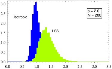
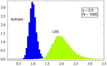
Figure 4: The distributions of the estimators ${\cal X}_{\rm iso}^{2}$ and ${\cal X}_{\rm LSS}^{2}$ for the cases $s=2.0$ and for $N=200,1000$ events. The distribution are the results of 10.000 monte-carlo simulation like described in the text.

In Figure 4 we show the distributions of the functions ${\cal X}_{\rm iso}^{2}$ and ${\cal X}_{\rm LSS}^{2}$ introduced in the previous section for $s=2.0$ and $N=200,1000$. It is clear that a few hundreds events are hardly enough to reliably distinguish the two models, while $N=\,$800–1000 should be more than enough to reject the hypothesis at 2-3$\,\sigma$, independently of the injection spectrum. Steeper spectra however slightly reduce the number of events needed for a given C.L. discrimination. Respect to the available data our results clearly show that AGASA statistics (only 32 data at $E\geq 5\times 10^{19}\,$eV in the published data set [17], some of which falling inside the mask) is too limited to draw any firm conclusion on the hypothesis considered.

4 Angular Power Spectrum

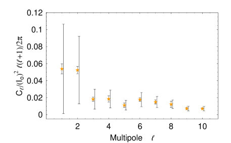
Figure 5: The first multipoles of the dimensionless angular power spectrum of the $5\times 10^{19}$ eV map from the fitting procedure; also showed, by comparison, the cosmic variance errors slightly shifted for clarity.

The previous forecast analysis is completely independent from an harmonic analysis of the anisotropies; however, a multipole decomposition and the related power spectrum calculation greatly helps in the understanding of the UHECRs anisotropies and, indeed, a dipole anisotropy study has been the aim of various works [18, 19, 20]; we cover the gap in this section.

In the following we will concentrate on the $E_{\rm cut}=5\times 10^{19}$ eV map; moreover, Auger is not expected to be very sensitive to multipoles higher than 10, even after ten years of operations, so we limit the analysis to the first few $l$.

The main problem in calculating the Spherical Harmonics expansion of the UHECRs map is the presence of the galactic avoidance zone; however, in the first few $l$’s the typical angular scale associated to the given multipole (of the order of $\sim\pi/l$) is larger of the average angular extension of the galactic cut so that an extrapolation in this zone is justified. We implement this method fitting to the UHECRs map the sum of the first harmonics till $l_{\rm max}$. The corresponding reconstructed map adding up to the first $l$=10 and $l$=2 harmonics is showed in Fig. 6 together with the original masked map.

Of course, filling the mask requires an extrapolation from the near regions and this is somewhat questionable in relation to the fact that some unknown cluster can be hidden behind our galaxy changing in principle all the multipoles pattern; a not well quantifiable error is indeed related to this ignorance though some more sophisticated astronomical analysis indicate that it is unlikely that relevant structures hide behind the galactic plane [21, 22, 23] so that at this angular resolution ($l=10$ corresponds to $180/10\approx 20^{\circ}$ resolution) an extrapolation is quite justified.

In this respect the situation is quite different from the CMB case where the anisotropies are isotropic and gaussian so that even a limited region of sky represents a fair statistical sample of the whole CMB sky, while the various multipoles are independent realization of the underlying random field. The UHECRs field is instead related to local and non-linear structures and it is then far from being gaussian; moreover the presence of possible unknown clusters in the avoidance zone introduces a correlation among the various mutipoles so that the naive error bars derived from the fit are not really trustable. We instead quantify the error looking at the spread of the best fit values obtained varying the degrees of freedom involved into the fit, related in its turn to the chosen $l_{\rm max}$. We varied $l_{\rm max}$ in the range 1-12 that we found to be optimal.

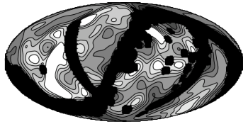
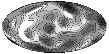
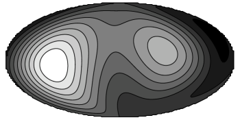
Figure 6: (a) The starting UHECRs map and mask in equatorial coordinates. (b) The reconstructed map from the first 10 multipoles. (c) As above for dipole+quadrupole.

The resulting angular power spectrum for the first 10 multipoles of the adimensional map $f_{\rm LSS}(\hat{\Omega},E_{\rm cut})/<\!\!{f}_{\rm LSS}\!\!>$ is shown in Fig. 5; note that the true errors are not affected by the cosmic variance given that we know the complete pattern of the angular anisotropies and not only their statistical properties. The hypothetical errors from the cosmic variance are, however, showed by comparison: as expected the true errors on the very wide structures of the dipole and quadrupole are quite small compared to cosmic variance; the errors, then, rapidly degrade when the scale related to the given $l$ approaches the size of the galactic cut so that already for $l=8-10$ the errors are almost comparable to the cosmic variance. As expected the dipole gives a prominent contribution though a similar power is predicted for the quadrupole; this is easily explained in terms of the original map where besides the Super-Galactic plane there is an important contribution from the P-P cluster, which induces a mixed dipolar-quadrupolar pattern. This contribution is almost an order of magnitude greater respect to the other multipoles so that, likely, it is also the dominant contribution in assessing the minimum statistics needed to detect the anisotropies like determined in the previous paragraphs. Since the dipole and quadrupole are the easiest anisotropies to look for in UHECR analyses, this result suggests that the $l$=1+$l$=2 pattern should slowly emerge from the cosmic rays data as the first detectable large scale anisotropy. Given the relevant role represented by the quadrupole and dipole we give in table 1 the expression of the $a_{lm}$ and the related errors, in equatorial coordinates. Finally, it is worth to notice the scale of the multipole anisotropies of the order $\sim 0.06$ that translates into an overall anisotropy of the order $\sim\sqrt{0.06}\approx 25\%$ in good agreement with what found with analysis of the full map.

$a_{lm}$	Re	Im
$a_{10}$	0.008 $\pm$ 0.027	…
$a_{11}$	0.230 $\pm$ 0.014	0.148 $\pm$ 0.039
$a_{20}$	-0.226 $\pm$ 0.049	…
$a_{21}$	-0.072 $\pm$ 0.035	0.093 $\pm$ 0.044
$a_{22}$	0.251 $\pm$ 0.042	-0.136 $\pm$ 0.021

Table 1: Low $l$ multipole moments in equatorial coordinates. $a_{l-m}$ moments are obtained through the reality condition $a_{l-m}=a_{lm}^{*}$.

As check of the method we perform an independent estimate of the power spectrum using the Master algorithm [24], a method typically employed in similar CMB analysis. This method is well suited for small scale anisotropies and is quite complementary to the fitting procedure; we verified that the two spectra superimpose and join smoothly making us confident on the reliability of the result.

5 Summary and conclusion

UHECRs offer the fascinating possibility to make astronomy with high energy charged particles; in particular, besides small scale clustering, a large scale anisotropy is expected correlating with the local cosmological LSS. However, we showed with a $\chi^{2}$ approach that a huge statistics of several hundreds data is required to start testing the model at Auger South.

Untill now, the lack of UHECR statistics has seriously limited the usefulness of such a kind of analysis. However, progresses are expected in forthcoming years. The Southern site of Auger is already taking data and, once completed, the total area covered will be of 3000 km², thus improving by one order of magnitude present statistics in a couple of years [25]. The idea to build a Northern Auger site strongly depends on the possibility to perform UHECR astronomy, for which full sky coverage is of primary importance. To this aim, the Japanese-American Telescope Array in the desert of Utah is expected to become operational by 2007 [26] offering almost an order of magnitude larger aperture per year than AGASA in the Northern sky.

References

- [1] K. Greisen, Phys. Rev. Lett. 16, 748 (1966).
- [2] G. T. Zatsepin and V. A. Kuzmin, JETP Lett. 4, 78 (1966) [Pisma Zh. Eksp. Teor. Fiz. 4, 114 (1966)].
- [3] K. Dolag, D. Grasso, V. Springel and I. Tkachev, JETP Lett. 79, 583 (2004) [Pisma Zh. Eksp. Teor. Fiz. 79, 719 (2004)] [astro-ph/0310902]; See also astro-ph/0410419.
- [4] G. Sigl, F. Miniati and T. Enßlin, Phys. Rev. D 70, 043007 (2004) [astro-ph/0401084]; see also astro-ph/0409098.
- [5] T. Antoni et al. [The KASCADE Collaboration], Astropart. Phys. 24, 1 (2005) [astro-ph/0505413].
- [6] M. Takeda et al. [AGASA collaboration], Astrophys. J. 522 225 (1999); [astro-ph/9902239]; See also M. Takeda et al., Proc. 27th ICRC, Hamburg, 2001.
- [7] R. U. Abbasi et al. [The HiRes Collaboration], Astrophys. J. 623, 164 (2005) [astro-ph/0412617].
- [8] B. Revenu [Pierre Auger Collaboration], in Proceedings of the 29th ICRC, (2005) Pune India.
- [9] J. W. Cronin, Nucl. Phys. Proc. Suppl. 28B, 213 (1992); see also http://www.auger.org/.
- [10] W. Saunders et al., Mon. Not. Roy. Astron. Soc. 317, 55 (2000) [astro-ph/0001117].
- [11] E. Waxman, K. B. Fisher and T. Piran, Astrophys. J. 483, 1 (1997) [astro-ph/9604005].
- [12] A. Smialkowski, M. Giller and W. Michalak, J. Phys. G 28, 1359 (2002) [astro-ph/0203337].
- [13] S. Singh, C. P. Ma and J. Arons, Phys. Rev. D 69, 063003 (2004) [astro-ph/0308257].
- [14] A. Cuoco, R. D. Abrusco, G. Longo, G. Miele and P. D. Serpico, JCAP 0601 (2006) 009 [astro-ph/0510765].
- [15] M. Kachelrieß P.D. Serpico, and M. Teshima, astro-ph/0510444.
- [16] P. Sommers, Astropart. Phys. 14, 271 (2001) [astro-ph/0004016].
- [17] N. Hayashida et al., Astron. J. 120, 2190 (2000) [astro-ph/0008102].
- [18] S. Mollerach and E. Roulet, JCAP 0508 (2005) 004 [astro-ph/0504630].
- [19] O. Deligny et al., JCAP 0410 (2004) 008 [astro-ph/0404253].
- [20] M. Kachelrieß and P. D. Serpico, astro-ph/0605462.
- [21] M. Rowan-Robinson et al., Mon. Not. Roy. Astron. Soc. 314, 375-397 (2000) [astro-ph/9912223].
- [22] O. Lahav, K. B. Fisher, Y. Hoffman, C. A. Scharf and S. Zaroubi, Astrophys. J. 423 (1994) L93 [astro-ph/9311059].
- [23] C. A. Scharf, Y. Hoffman, O. Lahav and Donald Lynden-Bell, Mon. Not. Roy. Astron. Soc. 256, 229-237 (1992).
- [24] E. Hivon et al. astro-ph/0105302.
- [25] X. Bertou [Pierre Auger Collaboration], astro-ph/0508466, in the Proceedings of the 29th ICRC, (2005) Pune India.
- [26] Y. Arai et al., Proceedings of 28th ICRC (2003), Tsukuba.