Dark Matter, Dark Energy and the solution of the strong CP problem

Abstract

The strong CP problem was solved by Peccei & Quinn by introducing axions, which are a viable candidate for Dark Matter (DM). Here the PQ approach is modified so to yield also Dark Energy (DE), which arises in fair proportions, without tuning any extra parameter. DM and DE arise from a single scalar field and, in the present ecpoch, are weakly coupled. Fluctuations have a fair evolution. The model is also fitted to WMAP first–year release, using a Markov Chain Monte Carlo technique, and performs as well as $\Lambda$CDM, coupled or uncoupled DE. Best–fit cosmological parameters for different models are mostly within 2–$\sigma$ level. The main peculiarity of the model is to favor high values of the Hubble parameter.

1 Introduction

Most cosmological data, including Cosmic Microwave Background (CMB) anisotropies, Large Scale Structure (LSS), as well as data on SNIa 1 , are fitted by a $\Lambda$CDM model with density parameters $\Omega_{DE}\simeq 0.7$, $\Omega_{m}\simeq 0.3$, $\Omega_{b}\simeq 0.04$ (for DE, non–relativistic matter and baryons), Hubble parameter $h\simeq 0.7$ (in units of 100 km/s/Mpc) and primeval spectral index $n_{s}\simeq 1$. However, the success of such $\Lambda$CDM does not hide its uneasiness. The parameters of standard CDM are still to be increased by one, in order to tune DE. Furthermore, if DE is ascribed to vacuum, this turns out to be quite a fine tuning. This conceptual problem was eased by dynamical DE models 2 ; 2a . They postulate the existence of an ad–hoc scalar field, self–interacting through a suitable effective potential, which depends, at least, on a further parameter (for SUGRA potential 2a here considered, this is an energy scale $\Lambda$ or an exponent $\alpha$).

Within the frame of dynamical DE models, we tried to take a step forward 3 . Instead of invoking an ad–hoc interaction, we refer to the field introduced by Peccei & Quinn (PQ) 4 to solve the strong–CP problem. Such scheme was already shown to yield DM 5 . In 3 we slightly modify the PQ scheme, replacing the Nambu–Goldstone (NG) potential introduced ad–hoc, by a tracker potential 2a so to yield also DE. This scheme solves the strong–CP problem even more efficiently than the original PQ model. We shall call this cosmology dual–axion model.

Its main peculiarity is naturally predicting DM–DE coupling. A number of authors discussed coupled DE models 6 , where a parameter $\beta$ fixes the coupling strength. Limits on $\beta$ arise from linear analysis, comparing predictions with CMB 9 or, more efficiently, from non–linear analysis. Non linearity boosts the effects of coupling 87 ; 88 .

Dual–axion model has several advantages both in respect to $\Lambda$CDM and ordinary or coupled dynamical DE: (i) it requires no fine tuning; (ii) it adds no parameter to the standard PQ scheme. DM and DE arise in fair proportions by fixing the energy scale $\Lambda$ of the tracker potential. Further, the model has no extra coupling parameter being the strength of the coupling set by the theory; (iii) it introduces no field or interaction, besides those required by particle physics. This scheme, however, leads to predictions (slightly) different from $\Lambda$CDM, for a number of observables. In principle, therefore, it can be falsified by data.

The only degree of freedom still allowed is the choice of the tracker potential. Up to now, the dual–axion scheme has been explored just in association with a SUGRA potential. In this case, it predicts a fair growth of density fluctuations, so granting a viable picture for the LSS.

The WMAP data on CMB anisotropies allow to submit the dual–axion model to further stringent tests, by comparing it with other cosmologies as $\Lambda$CDM, standard and interacting dynamical DE. None of the above models performs neatly better than the others. Apparently, the best fit is obtained by uncoupled DE with SUGRA potential.

2 A single scalar field to account for DM and DE

The solutions of the strong $CP$ problem proposed by PQ leads to one of the accepted models of DM. PQ suggested that $\theta$ parameter, in the effective lagrangian term

$${\cal L}_{\theta}={\alpha_{s}\over 2\pi}\theta\,G\cdot{\tilde{G}}$$ (1)

($\alpha_{s}$: strong coupling constant, $G$: gluon field tensor), causing $CP$ violations in strong interactions, is a dynamical variable. Under suitable conditions $\theta$ approaches zero in our epoch, so that the term (1) is suppressed, while residual $\theta$ oscillations yield DM 5 .

By adding to the Standard Model a global U(1) symmetry which is spontaneously broken at a scale $F_{PQ}$, $\theta$ is then the phase of a complex field $\Phi=\phi e^{i\theta}/\sqrt{2}$ which, falling into one of the degenerated minima of an NG potential

$$V(|\Phi|)=\lambda\,[\,|\Phi|^{2}-F_{PQ}^{2}\,]^{2}~{},$$ (2)

develops a vacuum expectation value $<\phi>=F_{PQ}$. The $CP$-violating term, arising around quark-hadron transition when $\bar{q}q$ condensates break the chiral symmetry, reads

$$V_{1}=\left[\sum_{q}\langle 0(T)|{\bar{q}}q|0(T)\rangle m_{q}\right]~{}(1-\cos\theta)$$ (3)

($\sum_{q}$ extends over all quarks), so that $\theta$ is no longer arbitrary, but shall be ruled by a suitable equation of motion. The term in square brackets, at $T\simeq 0$, approaches $m_{\pi}^{2}f_{\pi}^{2}$ ($m_{\pi}$ and $f_{\pi}$: $\pi$–meson mass and decay constant).

In the next Sections, we will discuss the work in 3 , where the NG potential (2) is replaced by a tracker potential. Then, instead of settling on a value $F_{PQ}$, $\phi$ continues to evolve over cosmological times, at any $T$. As in the PQ case, the potential involves a complex field $\Phi$ and is $U(1)$ invariant.

At variance from the PQ case, however, the $\theta$ evolution starts and continues while also $\phi$ is still evolving. This goes on until our epoch, when $\phi$ is expected to account for DE, while, superimposed to such slow evolution, faster transversal $\theta$ oscillations occur, accounting for DM. As it can be expected, however, DM and DE are dynamically coupled, although this coupling weakens as we approach the present era.

2.1 Lagrangian theory

In the dual–axion model we start from the lagrangian ${\cal L}=\sqrt{-g}\{g_{\mu\nu}\partial_{\mu}\Phi\partial_{\nu}\Phi-V(|\Phi|)\}$ which can be rewritten in terms of $\phi$ and $\theta$, adding also the term breaking the $U(1)$ symmetry, as follows:

$${\cal L}=\sqrt{-g}\big{\{}(1/2)\,g_{\mu\nu}\big{[}\,\partial_{\mu}\phi\partial_{\nu}\phi+\phi^{2}\partial_{\mu}\theta\partial_{\nu}\theta\,\big{]}-V(\phi)-m^{2}(T,\phi)\phi^{2}(1-\cos\theta)\big{\}}~{}.$$ (4)

Here $g_{\mu\nu}$ is the metric tensor. We shall assume that $ds^{2}=g_{\mu\nu}dx^{\mu}dx^{\nu}=a^{2}(d\tau^{2}-\eta_{ij}dx_{i}dx_{j})$, so that $a$ is the scale factor, $\tau$ is the conformal time; greek (latin) indeces run from 0 to 3 (1 to 3); dots indicate differentiation with respect to $\tau$. The mass behavior for $T\sim\Lambda_{QCD}$ will be detailed in the next Section. The equations of motion read

$$\ddot{\theta}+2(\dot{a}/a+\dot{\phi}/\phi)~{}\dot{\theta}+m^{2}a^{2}\sin\theta=0~{},$$ (5)

$$\ddot{\phi}+2(\dot{a}/a)\,\dot{\phi}+a^{2}V^{\prime}(\phi)=\phi\,\dot{\theta}^{2},$$ (6)

while the energy densities $\rho_{\theta,\phi}=\rho_{\theta,\phi;kin}+\rho_{\theta,\phi;pot}$ and pressures $p_{\theta,\phi}=\rho_{\theta,\phi;kin}-\rho_{\theta,\phi;pot}$, under the condition $\theta\ll 1$, are obtainable from

$$\rho_{\theta,kin}={\phi^{2}\dot{\theta}^{2}/2a^{2}}~{},~{}~{}\rho_{\theta,pot}=m^{2}(T,\phi)\phi^{2}\theta^{2}/2~{},~{}~{}$$

$$\rho_{\phi,kin}={\dot{\phi}^{2}/2a^{2}}~{},~{}~{}\rho_{\phi,pot}=V(\phi)~{}.~{}~{}~{}~{}~{}~{}~{}~{}~{}~{}~{}$$ (7)

2.2 Axion mass

According to eq. (5), the axion field begins to oscillate when $m(T,\phi)a\simeq 2(\,{\dot{a}/a}+{\dot{\phi}/\phi}\,)$. In the dual–axion model, just as for PQ, axions become massive when the chiral symmetry is broken by the formation of the $\bar{q}q$ condensate at $T\sim\Lambda_{QCD}$. Around such $T$, therefore, the axion mass grows rapidly. In the dual–axion model, however, a slower growth takes place also later, because of the evolution of $\phi$. Then $m(T,\phi)$ is

$$m_{o}(\phi)={m_{\pi}f_{\pi}/\phi}=(0.0062/\phi)~{}{\rm GeV}~{}.$$ (8)

Since $\phi\sim m_{p}$ today, the axion mass is now $m_{o}\sim 5\cdot 10^{-13}$eV, while, according to 8 , at high $T:$

$$m(T,\phi)\simeq 0.1\,m_{o}(\phi)(\Lambda_{QCD}/T)^{3.8}~{}~{}.$$ (9)

This expression must be interpolated with eq. (8), to study the fluctuation onset for $T\sim\Lambda_{QCD}$. Details on interpolation can be found in 3 .

2.3 The case of SUGRA potential

When $\theta$ performs many oscillations within a Hubble time, then $\langle\rho_{\theta,kin}\rangle\simeq\langle\rho_{\theta,pot}\rangle$ and $\langle p_{\theta}\rangle\simeq 0$. By using eqs. (5),(6),(7), it is easy to see that

$$\dot{\rho}_{\theta}+3H\rho_{\theta}={\dot{m}\over m}\,\rho_{\theta}~{},~{}\dot{\rho}_{\phi}+3H(\rho_{\phi}+p_{\phi})=-{\dot{m}\over m}\rho_{\theta}~{}.$$ (10)

When $m$ is given by Eq (9) , $\dot{m}/m=-\dot{\phi}/\phi-3.8\,\dot{T}/T$. At $T\simeq 0$, instead, $\dot{m}/m\simeq-\dot{\phi}/\phi$. Here below, the indices _θ, _ϕ will be replaced by ${}_{DM},_{DE}$. Eqs. (10) show an energy exchange between DM and DE. The former eq. (10) can then be integrated, yielding $\rho_{DM}\propto m/a^{3}$. This law holds also when $T\ll\Lambda_{QCD}$, and then the usual behavior $\rho_{DM}\propto a^{-3}$ is modified, becoming $\rho_{DM}a^{3}\phi\simeq{\rm const}.$ Let us now assume that the potential reads

$$V(\phi)=(\Lambda^{\alpha+4}/\phi^{\alpha})\exp(4\pi\phi^{2}/m_{p}^{2})$$ (11)

(no $\theta$ dependence); in the radiative era, it will then be $\phi^{\alpha+2}=g_{\alpha}\Lambda^{\alpha+4}a^{2}\tau^{2}~{},$ with $g_{\alpha}=\alpha(\alpha+2)^{2}/4(\alpha+6)$. This tracker solution holds until we approach the quark–hadron transition. Then, in Eq. (6), the DE–DM coupling term, $\phi\dot{\theta}^{2}$, exceeds $a^{2}V^{\prime}$ and we enter a different (tracking) regime.

Figure 1: Left and centre: energy densities $\rho_{i}$ and density parameters $\Omega_{i}$ vs. scale factor a.

This is shown in detail in the left plot (panel (a)) of Fig.(1) obtained for $\Omega_{m}=0.3$, $\Omega_{b}=0.03$ and Hubble constant $h=0.7$ (in units of 100 km/s/Mpc). Panel (b) then shows the low–$z$ behavior, since DE energy density exceeds radiation ($z\simeq 100$) and then overcomes baryons ($z\simeq 10$) and DM ($z\simeq 3$). In the central plot of Fig.(1) a landscape picture for all energy densities $\rho_{i}$ ($i=r,~{}b,~{}\theta,~{}\phi$, i.e. radiation, baryons, DM, DE), down to $a=1$ (top panel) and the related behaviors of the density parameters $\Omega_{i}$ (bottom panel) are shown.

In general, once $\Omega_{DE}$ (at $z=0$) is assigned, a model with dynamical (coupled or uncoupled) DE is not yet univocally determined. For instance, the potential (11) depends on the parameters $\alpha$ and $\Lambda$ and one of them can still be arbitrarily fixed. In dual–axion model such arbitrariness no longer exists. The observational value of the densities in the world forces the scale factor $a_{h}$ when oscillations start to lay about the quark–hadron transition, while also $\Lambda$ is substantially fixed. For $\Omega_{DM}=0.27$ we obtain $\Lambda\simeq 1.5\cdot 10^{10}$GeV and $a_{h}\sim 10^{-13}$. But, when $\Omega_{DM}$ goes from 0.2 to 0.4, $\log_{10}(\Lambda/{\rm GeV})$ (almost) linearly runs in the narrow interval 10.05–10.39 , while $a_{h}$ steadily lays at the eve of the quark–hadron transition. For more details on this point see 3 .

2.4 Evolution of inhomogeneities

Besides of predicting fair ratios between the world components, a viable model should also allow the formation of structures in the world.

The dual–axion model belongs to the class of coupled DE models treated by Amendola 10 , with a time dependent coupling $C(\phi)=1/\phi$. Fluctuations evolution is then obtained by solving the equations in 10 , with the above $C(\phi)$. The behavior shown in the right plot of Fig.(1) is then found. The bottom panel compares DM fluctuation evolutions in the the dual–axion model (solid curves), with those in an analogous $\Lambda$CDM model (long–dashed curves) and in a coupled DE model with constant coupling $C\simeq\langle C(\phi)\rangle$ (short–dashed curves). As shown by the plots, the overall growth, from recombination to now is similar in dual–axion and $\Lambda$CDM models, being quite smaller than in DE models with constant coupling. The differences of dual–axion from $\Lambda$CDM are: (i) objects form earlier and (ii) baryon fluctuations keep below DM fluctuations until very recently.

3 Comparison with WMAP data

Table 1: SUGRA parameters for uncoupled DE (left), constant coupling (center) and $\phi^{-1}$ model (right).

uncoupled SUGRA
$x$	$\langle x\rangle$	$\sigma_{x}$
$\Omega_{b}h^{2}$	0.025	0.001
$\Omega_{DM}h^{2}$	0.12	0.02
$h$	0.63	0.06
$\tau$	0.21	0.07
$n_{s}$	1.04	0.04
$A$	0.97	0.13
$\lambda$	3.0	7.7

SUGRA with C=const
$x$	$\langle x\rangle$	$\sigma_{x}$
$\Omega_{b}h^{2}$	0.024	0.001
$\Omega_{DM}h^{2}$	0.11	0.02
$h$	0.74	0.11
$\tau$	0.18	0.07
$n_{s}$	1.03	0.04
$A$	0.92	0.14
$\lambda$	-0.5	7.6
$\beta$	0.10	0.07

SUGRA with C=$\phi^{-1}$
$x$	$\langle x\rangle$	$\sigma_{x}$
$\Omega_{b}h^{2}$	0.025	0.001
$\Omega_{DM}h^{2}$	0.11	0.02
$h$	0.93	0.05
$\tau$	0.26	0.04
$n_{s}$	1.23	0.04
$A$	1.17	0.10
$\lambda$	4.8	2.4

We have tested the dual–axion model against CMB data, together with other dynamical DE cosmologies. We used the Markov Chain Monte Carlo program 11 also used in the original analysis of WMAP first–year data 12 to constrain a flat $\Lambda$CDM in respect to six parameters: $\Omega_{b}h^{2}$, $\Omega_{m}h^{2}$, $h$, $n_{s}$, the fluctuation amplitude $A$ and the optical depth $\tau$.

In our analysis, three classes of DE were considered: (i) uncoupled SUGRA DE, requiring an extra parameter $\lambda=\log_{10}(\Lambda/{\rm GeV})$, the energy scale in the potential (12). (ii) Constant coupling SUGRA DE, with a further parameter $\beta\propto C$. (iii) Coupled models with $C=\phi^{-1}$, keeping just $\lambda$ as a free parameter. The (iii) class of model includes the dual–axion case, for which, however $\lambda$ is set by the requirement that $\Omega_{DE}$ lays in a fair range so that $\lambda$ and $\Omega_{DE}$, are no longer independent. Then, we tested whether data constrain $\lambda$ into a fair region, turning a generic $\phi^{-1}$ model into a dual–axion model.

The basic results are summarized in the Table 1. For each model we list the expectation values $\langle x\rangle$ of each parameter $x$ and the related variance $\sigma_{x}$.

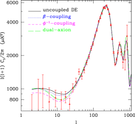
Figure 2: $C_{l}^{T}$ spectra for the best fit SUGRA (solid line), constant coupling (dotted line), $\phi^{-1}$–coupling (dashed) and dual–axion (dot–dashed) models.

A first point worth outlining is that SUGRA (uncoupled) models, bearing precise advantages in respect to $\Lambda$CDM, are consistent with WMAP data.

In uncoupled or costant coupling SUGRA models opacity ($\tau$) is pushed to values even greater than in $\Lambda$CDM 13 . Greater $\tau$’s have an indirect impact also on $\Omega_{b}h^{2}$ whose best–fit value becomes greater, although consistent with $\Lambda$CDM within 1–$\sigma$.

Parameters are more strongly constrained in $\phi^{-1}$ models. In particular, WMAP data yield constraints on $\lambda$ for $\phi^{-1}$ models and the 2–$\sigma$ $\Lambda$–interval ranges from $\sim 10$ to $\sim 3\cdot 10^{10}$GeV, so including the dual–axion model. The main puzzling feature of $\phi^{-1}$ models is that large $h$ is favored: the best–fit 2–$\sigma$ interval does not extend below 0.85 . The problem is more severe for dual–axion $\lambda$’s values. This model tends to displace the first $C_{l}^{T}$ peak to greater $l$ (smaller angular scales) as coupling does in any case does. The model, however, has no extra coupling parameter and the intensity of coupling is controlled by the scale $\Lambda$. Increasing this scale requires a more effective compensation and greater values of $h$ are favored. This effect appears related to the choice of SUGRA potentials, which is just meant to provide a concrete framework for the dual axion model.

The fits to WMAP data yield similar $\chi^{2}$ for all models ranging from 1.064 (no coupling) to 1.074 ($\phi^{-1}$ coupling) 3 . Fig. (2) compares the $C_{l}^{T}$ spectra for all best–fit models (apart of $\Lambda$CDM). At large $l$ all models yield similar behaviors and this is why no model category prevails.

4 Conclusions

Axions have been a good candidate for DM since the late Seventies. They arise from the solution of the strong CP problem proposed by PQ. Here we showed that their model has a simple and natural generalization that also yields DE adding no parameter to the standard PQ scheme. A complex scalar fields $\Phi$, arising in the solution of the strong CP problem, accounts for both DE and DM: as in the PQ model, in eq. (1) $\theta$ is turned into a dynamical variable, the phase of $\Phi$. Here, however, instead of taking a constant value, $|\Phi|$ increases in time, approaching $m_{p}$ by our cosmic epoch, when it is DE; meanwhile, $\theta$ is driven to approach zero, still performing harmonic oscillations which are axion DM. The critical scale factor $a_{h}$ when oscillations start, lays at the eve of the quark–hadron transition, because of the rapid increase of the axion mass $m(T,\phi)$. The scale $a_{h}$ is essentially model independent and no appreciable displacement can be expected just varying $\Omega_{DM}$ while rather high values of $h$ tend to be preferred. This implies that the scale $\Lambda$ in the SUGRA potential is almost model independent 3 . Therefore, the unique setting of $\Omega_{DM}$ fixes $\Lambda$ also providing DM and DE in fair proportions and simultaneously solving the strong $CP$ problem.

The fits to WMAP first–year data of uncoupled, constant–coupling and $\phi^{-1}$ SUGRA models yield similar $\chi^{2}$’s. At variance from other models, in $\phi^{-1}$ models, CMB data constrain $\Lambda$ and it is significant that the allowed range includes values consistent with the dual–axion model.

References

- (1) Tegmark M., et al. 2004, Phys.Rev. D69, 10350; De Bernardis et al., 2000 Nature 404, 955; Hanany S. et al, 2000, ApJ 545, L5; Halverson N.W. et al. 2002, ApJ 568, 38; Percival W.J. et al., 2002, MNRAS, 337, 1068 , Riess, A.G. et al., 1998, Aj 116, 1009; Perlmutter S. et al., 1999, Apj, 517, 565
- (2) Wetterich C., 1995 A&A 301, 32; Ratra B. & Peebles P.J.E., 1988, Phys.Rev.D, 37, 3406; Ferreira G.P. & Joyce M. 1998 Phys.Rev.D 58, 023503
- (3) Brax, P. & Martin, J., 1999, Ph.Lett. B468, 40; Brax P., Martin J., Riazuelo A., 2000, P.R. D62, 103505
- (4) Mainini R. & Bonometto S.A, 2004, Phys.Rev.Lett. 93, 121301; Mainini R., Colombo L.P.L., & Bonometto S.A, 2005, AJ 632, 691
- (5) Peccei R.D. & Quinn H.R. 1977, Phys.Rev.Lett. 38, 1440; Kim J.E. 1979, Phys.Rev.Lett. 43, 103.
- (6) Weinberg S. 1978, Phys.Rev.Lett. 40, 223; Wilczek F. 1978, Phys.Rev.Lett. 40, 279; Preskill J. et al 1983, Phys.Lett B120, 225; Abbott L. & Sikivie P. 1983 Phys.Lett B120, 133; Dine M. & Fischler 1983 Phys.Lett B120, 137; Turner M.S. 1986 Phys.Rev.D 33, 889
- (7) Amendola L. 2000, Phys.Rev D62, 043511; Gasperini M., Piazza F. & Veneziano G., 2002, Phys. Rev. D65, 023508; Perrotta F. & Baccigalupi C., 2002, Phys. Rev. D65, 123505
- (8) Amendola L. & Quercellini C., 2003, Phys. Rev. D68, 023514
- (9) Macciò A., Quercellini C., Mainini R., Amendola L., Bonometto S.A. 2004, Phys. Rev. D69, 123516
- (10) Mainini R., 2005, Phys.Rev.D 72, 083514; Mainini R. & Bonometto S., 2006, Phys.Rev. D74, 043504
- (11) Kolb R.W. & Turner M.S. 1990 The Early Universe, Addison Wesley, and references therein
- (12) Amendola L., 2004, Phys.Rev. D69, 103524
- (13) Knox L., Christensen, N. & Skordis C. 2001, ApJ 63, L95; Lewis, A. & Bridle, S. 2002, Phys.Rev. D 66, 103511; Kosowsky A., Milosavljevic M. & Jimenez R. 2002, Phys.Rev.D 66, 63007
- (14) Spergel D.N. et al., 2003, ApJ Suppl. 148, 175
- (15) Corasaniti P.S., et al. 2004, Phys. Rev. D70, 083006 astro–ph/0406608
- (16) Weller J. & Lewis A.M. 2003, MNRAS, 346, 987
- (17) Colombo L.P.L., Mainini R. & Bonometto S.A. 2003, in proceedings of Marseille 2003 Meeting, ’When Cosmology and Fundamental Physics meet’