Type Ia Supernova Light Curves

Abstract

The diversity of Type Ia supernova (SN Ia) photometry is explored using a grid of 130 one-dimensional models. It is shown that the observable properties of SNe Ia resulting from Chandrasekhar-mass explosions are chiefly determined by their final composition and some measure of “mixing” in the explosion. A grid of final compositions is explored including essentially all combinations of ⁵⁶Ni, stable “iron”, and intermediate mass elements that result in an unbound white dwarf. Light curves (and in some cases spectra) are calculated for each model using two different approaches to the radiation transport problem. Within the resulting templates are models that provide good photometric matches to essentially the entire range of observed SNe Ia. On the whole, the grid of models spans a wide range in $B$-band peak magnitudes and decline rates, and does not obey a Phillips relation. In particular, models with the same mass of ⁵⁶Ni show large variations in their light curve decline rates. We identify and quantify the additional physical parameters responsible for this dispersion, and consider physically motivated “cuts” of the models that agree better with the Phillips relation, discussing why nature may have preferred these solutions. For example, models that produce a constant total mass of burned material of 1.1 $\pm 0.1$ $\mathrm{M}_{\odot}$ do give a crude Phillips relation, albeit with much scatter. If one further restricts that set to models that make 0.1 to 0.3 $\mathrm{M}_{\odot}$ of stable iron and nickel isotopes, and then mix the ejecta strongly between the center and 0.8 $\mathrm{M}_{\odot}$, reasonable agreement with the Phillips relation results, though still with considerable spread. We conclude that the supernovae that occur most frequently in nature are highly constrained by the Phillips relation and that a large part of the currently observed scatter in the relation is likely a consequence of the intrinsic diversity of these objects.

1. INTRODUCTION

The application of Type Ia supernovae (SNe Ia) to cosmological distance determination has yielded revolutionary insights into the structure and composition of the universe (Perlmutter et al., 1999; Riess et al., 1998). The utility of such explosions is based upon two empirical observations. First, that Type Ia supernovae are, for the most part, approximate standard candles, even without any corrections being applied. This probably reflects their common origin in the explosion of a white dwarf of standard mass (see review by Hillebrandt & Niemeyer, 1999). Second, a large part of the residual diversity in peak brightness can be corrected for by use of either light curve template fitting or observed correlations between light curve decline rate and peak brightness - the so called “Phillips Relation”(Phillips, 1993), or “width-luminosity relation” (henceforth WLR).

While the empirical relation between brightness and width has worked well for most purposes, as we move into an era of “precision cosmology”, one must feel increasing unease at the lack of an agreed upon standard model for how Type Ia supernovae explode and the possibility that evolutionary or environmental factors may erode accuracy at large distances. If the mass of ⁵⁶Ni made in a supernova is the dominant physical parameter affecting both brightness and light curve shape, what are the magnitude and direction of other possible parameters of the explosion such as kinetic energy, intermediate mass element production, stable iron production and mixing? And if, as we shall find, not all physically plausible models obey a WLR, why has nature chosen to realize frequently a particular subset? That is, what does the WLR tell us, not just about cosmology, but about supernova models? If one can make progress on both these questions, then it may be possible to derive more rigorous and quantitative tools for using Type Ia supernovae for distance determination. That is the long term goal of our investigation.

In this paper, we introduce a simple parameterized approach to computing SN Ia explosions and use it to generate a large grid of one-dimensional models. For each model, we calculate synthetic broadband light curves and examine the relationship between peak $B$ magnitude and $B$-band decline rate. Such an approach allows us to study the physical parameters affecting the light curves of SNe Ia and the WLR. Several previous theoretical studies have performed similar investigations for a given set of models (Khokhlov et al., 1993; Höflich et al., 1996, 1998; Pinto & Eastman, 2001; Höflich et al., 2002; Mazzali et al., 2001). These studies, however, were typically confined to a certain class (or classes) of theoretical explosion paradigms. In this study, rather than adopt a specific theoretical framework, we take a general and exhaustive approach by simulating the full range of final ejecta structures conceivably arising from the disruption of a Chandrasekhar-mass carbon-oxygen white dwarf.

2. A SIMPLE MODEL FOR THE EXPLOSION

2.1. Construction and Parameters of the Model

Here a simple ansatz for the explosion model is introduced that turns out to work surprisingly well. It is assumed that all SNe Ia start from a common point, a 1.38 $\mathrm{M}_{\odot}$ carbon oxygen white dwarf with a central density $2-3\times 10^{9}$ g cm^-3. Burning, which may be quite complicated, turns some part of that fuel into ash and deposits an internal energy in the dwarf equal to the difference in nuclear binding energy between the initial and final compositions. This composition is imprinted on the white dwarf and, in our calculations, the corresponding change in nuclear binding energy is deposited uniformly throughout its mass. The white dwarf expands to infinity with a velocity distribution determined by that energy. The ⁵⁶Ni and ⁵⁶Co decay, and the time-dependent radiation transport is calculated.

The major assumption that facilitates the calculation is that the energy deposition is shared globally. This is clearly true in spherically symmetric deflagration models, since sound waves move much faster than the flame and share the overpressure created by the burning with the rest of the star. It is also true in detonations except for a thin layer near the surface. Throughout most of the star, the passage of a detonation wave changes the composition and internal energy. Most acceleration occurs afterwards. After expansion of a factor of one million (before it can be seen), and the development of a velocity field that must increase with Lagrangian mass, the results are the same as achieved by a simple composition swap and artificial energy deposition. Perhaps the best validation of the model is that it works. Calculations given in § 4.2 and § 4.3 show that the multi-band photometry of models calculated this way agrees, both with previous detailed numerical simulations of the explosion, like the well-studied Model W7, and with a diverse set of observed supernovae.

However, the simple model has one basic shortcoming. It will turn out that “mixing” - just how a given composition is distributed in velocity - is an important parameter of the problem. It is this information that must eventually be provided by a full, first-principle’s calculation. Buried within this mixing parameter is also information about the possible asymmetry of the explosion. Such simulations must ultimately be three dimensional. However, the present models are as “physical” as most other one-dimensional approximations that make assumptions about flame speeds, transitions to detonation, metallicity, etc.

The dominant products of burning are assumed to be: i) ⁵⁶Ni; ii) “stable iron”, that is all the other nuclei in the iron group, chiefly ⁵⁴Fe and ⁵⁸Ni; and iii) intermediate mass elements - Si, S, Ar, Ca, henceforth referred to as “IME”. In the latter group Si and S are most abundant and, for making energy, most important, but Ca is important for the spectrum. These are the parameters of the solution. Here IME ratios are adopted from Model DD4 of Woosley & Weaver (1994): by mass Si (53%), S (32%), Ar (6.2 %) and Ca (8.3%). Solar ratios (Lodders, 2003) would not have been much different: Si (58%), S (29%), Ar (7.7%), and Ca (5.2%). There is some physical motivation for this as well. At the temperatures where carbon and oxygen burn to silicon, 3 - 5 $\times 10^{9}$ K, quasi-equilibrium favors an approximately solar abundance set (Woosley et al., 1973). Stable iron is taken in the calculation to be ⁵⁴Fe. A further refinement in which stable iron is split into ⁵⁴Fe and ⁵⁸Ni could easily be done, but would add an additional parameter without greatly affecting the light curve.

The relative amounts of these three sets of burning products reflect specific physical processes in the star and play a unique role in making the light curve and spectrum. “Stable iron” is a measure of burning at temperatures and densities so high (T $\lower 0.43057pt\hbox{\hbox to0.0pt{\raise 2.58334pt\hbox{\hskip 1.29167pt{{$\scriptscriptstyle>$}}}\hss} \kern-1.72218pt{{$\scriptscriptstyle\sim$}}}5\times 10^{9}$ K; $\rho\lower 0.43057pt\hbox{\hbox to0.0pt{\raise 2.58334pt\hbox{\hskip 1.29167pt{{$\scriptscriptstyle>$}}}\hss} \kern-1.72218pt{{$\scriptscriptstyle\sim$}}}10^{8}$ g cm^-3) that nuclear statistical equilibrium is attained and accompanied by electron capture. To some extent, stable iron is also a function of the initial metallicity of the star (Timmes et al., 2003). Stable iron-group isotopes contribute to the opacity and explosion energy, but not to the later energy generation that makes the light curve. A higher ignition density, which might reflect a lower accretion rate, increases the production of stable iron. The most natural location for stable iron is in the center of the supernova where the density was the highest, but iron will also exist at a level of about 5% (Z/$Z_{\odot}$) by mass in the ⁵⁶Ni layer. This is a consequence of the ²²Ne present in the initial composition from helium burning, and the number is sensitive (linearly) to the metallicity.

The double magic nucleus ⁵⁶Ni is always the dominant product of nucleosynthesis starting from a fuel with equal numbers of neutrons and protons (like ¹²C and ¹⁶O) when nuclear statistical equilibrium is attained. Its abundance therefore reflects the extent of nuclear burning above $5\times 10^{9}$ K at densities low enough that electron capture is negligible. Without doubt, it is the key player in the SN Ia light curve. Along with its decay product ⁵⁶Co, it powers the light curve and also contributes to the opacity and explosion energy. The most natural location for the ⁵⁶Ni is also deep inside the star just outside the stable iron. However, turbulence, instabilities in the explosion, and perhaps delayed detonation may lead to some of the ⁵⁶Ni (and to some extent, stable iron) being “mixed” far out, perhaps even to the surface.

IME are made when the density in the burning region declines to about 10⁷ g cm^-3. There, the heat capacity of the radiation field keeps the burning from going all the way to equilibrium. While these elements cause prominent line features in the SN Ia spectrum, their opacities and emissivities are not as important to the light curve as are those of nickel, cobalt and iron. Their production does, however, contribute to the explosion energy. The most natural location of IME is in the outer layers of the supernova, although instabilities and delayed detonation can lead to mixing among the layers in velocity space.

Given an initial white dwarf, the free parameters of the calculation are thus $M_{\mathrm{Ni}}$, $M_{\mathrm{Fe}}$, and $M_{\mathrm{IME}}$. To this list one must also add “mixing”, which is harder to quantify. The carbon-to-oxygen ratio and the white dwarf binding energy (or equivalently ignition density) also affect the overall energetics of the explosion. Burning carbon releases a little more energy than burning oxygen and a more tightly bound white dwarf requires more energy to give a certain expansion speed. Here we assume a standard, near Chandrasekhar-mass white dwarf (1.38 $\mathrm{M}_{\odot}$) composed of equal amounts of carbon and oxygen (50% by mass fraction of each) with an ignition density of $2.9\times 10^{9}$ g cm^-3. This corresponds to a net binding energy (internal energy plus gravitational binding energy) of $4.62\times 10^{50}$ erg (Coulomb corrections are neglected in this study). The ignition density cannot be much greater than this or the production of rare neutron-rich species will exceed the Galactic inventory as represented by the sun (Woosley, 1997). The runaway will not ignite at densities below about $2.5\times 10^{9}$ g cm^-3 for reasonable choices of the electron screening function.

The energy of the explosion is determined by the energy released in the nuclear burning. The asymptotic kinetic energy of the SN Ia explosion is directly related to the amount of material burned in the explosion, in particular, for a starting composition of 50% C and 50% O,

$$E_{K}=1.56M_{\mathrm{Ni}}+1.74M_{\mathrm{Fe}}+1.24M_{\mathrm{IME}}-E_{g}+E_{int}$$ (1)

where $E_{g}=3.35$ B (here 1 B = 1 Bethe = 10⁵¹ erg) is the gravitational binding energy and $E_{int}=2.89$ B, the internal energy of the progenitor white dwarf. If the composition were 30% C and 70% O, the yields would be about 7% less for Ni and Fe and 9% less for Si - Ca. A similar change in the opposite direction occurs for an oxygen-rich initial composition - 70% O and 30% C.

This energy is deposited uniformly (as a certain number of erg g^-1) throughout the entire mass of the initial white dwarf and the composition of the layers changed appropriately (e.g., Fig. 1 for an explosion that made 0.7 $\mathrm{M}_{\odot}$ of ⁵⁶Ni, 0.1 $\mathrm{M}_{\odot}$ of ⁵⁴Fe and 0.3 $\mathrm{M}_{\odot}$ of Si-Ca), The ensuing evolution is followed using the kepler implicit hydrodynamics code (Weaver, Zimmerman, & Woosley, 1978; Woosley et al., 2002). After less than a minute (star time), the explosion is homologously coasting and can be mapped into either of the radiation codes discussed in § 3.1 or § 3.2. The hydrodynamical calculation also takes less than one minute on a desktop processor, thus allowing a large number of models with carefully controlled properties to be generated.

2.2. Mixing

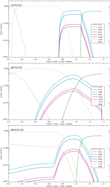
Figure 1.— Various parameterized mixing prescriptions applied to the model with 0.7 $\mathrm{M}_{\odot}$ of ${}^{56}\mathrm{Ni}$, 0.1 $\mathrm{M}_{\odot}$ of stable iron, and 0.3 $\mathrm{M}_{\odot}$ of IME. The remainder is carbon and oxygen in equal (50%) amounts by mass. The lines for C and O lie on top of each other in the figure. Model C070101 is very mildly mixed corresponding to moving boxcar average with a window of 0.02 $\mathrm{M}_{\odot}$ applied three times. In Model M070103, the same star and composition has been mixed with the same 0.02 $\mathrm{M}_{\odot}$ interval 50 times. Model MC070103 is extensively mixed inside 0.8 $\mathrm{M}_{\odot}$ and mildly mixed outside (see text).

“Mixing” is a general term referring to the fact that the ejected composition is not stratified into shells of pure ashes from a given burning process - here ⁵⁴Fe, ⁵⁶Ni, Si-Ca, and CO - but has somehow become blended in velocity space. Mixing occurs at some level simply because the burning temperature is continuous. Carbon and oxygen don’t burn only to Si-Ca or ⁵⁶Ni, but, at some temperatures, to a mixture of both. Stable iron may be present in the ⁵⁶Ni layer if the star had an appreciable (especially super-solar) metallicity. The most difficult mixing to quantify however, is a consequence of the inherently multi-dimensional nature of the burning which, from start to finish, is Rayleigh-Taylor unstable and turbulent. Particular models like gravitationally confined detonation (Plewa et al., 2004; Röpke, Woosley, & Hillebrandt, 2006) even have most of the burning starting at the surface and moving inwards.

A great variety of mixing is, in principle, possible and to the extent that our results turn out to be sensitive to mixing, the simple ansatz employed for the explosion is questionable. However, there are some general rules that mixing should obey. First, mass and energy are conserved, so the dynamics of the explosion, including the density profile in the coasting configuration is probably not affected very much. Second, the angle-averaged atomic weight of the ejecta probably decreases from the middle outwards. That is ⁵⁶Ni and stable iron are concentrated more towards the center, carbon and oxygen on the outside, and Si-Ca, in between. Third, the neutron excess, $\eta=\Sigma(N-Z)X/A$, also decreases from the center to the surface.

A one-dimensional treatment of mixing may not be so bad, as far as the radiative transfer is concerned. The observed light curve is the emission integrated over the entire star. Angle-dependent mixing can certainly have consequences for individual spectral lines, but has a smaller effect on the photometry. This motivates the treatment of mixing as a parameterized one-dimensional process that stirs, but does not homogenize the composition. Here, that is accomplished by a running boxcar average of abundances in a certain mass interval moved from the center to surface of the star. In a typical mixing operation, starting with zone 1, the composition in the next 0.02 $\mathrm{M}_{\odot}$ outwards is homogenized. One then moves to zone 2 and does the same operation, and so on until the stellar surface is reached. If more mixing is desired, then either the mass interval is widened or the operation repeated, from center to surface, multiple times. The latter approach was adopted here. Mildly and moderately mixed versions of a sample model are shown in Fig. 1.

2.3. Model Nomenclature

Models are named here according to their composition and the mixing prescription employed. Model Cxxyyzz is a “mildly mixed” model with xx/10 solar masses of ⁵⁶Ni, yy/10 solar masses of stable iron, zz/10 solar masses of IME (Si-Ca), and 1.38 - (xx+yy+zz)/10 solar masses of carbon and oxygen. Prior to mixing, unless otherwise mentioned, the ordering of the composition is stable iron (center), ⁵⁶Ni next, and (Si-Ca) farthest out, followed by unburned carbon and oxygen. By mild mixing (Fig. 1) we mean specifically that a moving interval of mass of 0.02 $\mathrm{M}_{\odot}$ was mixed from center to surface three times. “Moderately mixed” models, Mxxyyzz, which are most frequently employed in this paper, apply the same moving boxcar average 50 times. “Highly mixed” models, MMxxyyzz, apply the same moving boxcar average 200 times.

A finer grid of the M-series models was also prepared for highlighting a restricted range of burned mass (§ 7.2), 1.0 and 1.1 $\mathrm{M}_{\odot}$; ${}^{56}\mathrm{Ni}$ masses, 0.4 to 0.9 $\mathrm{M}_{\odot}$  and stable iron masses, 0 - 0.3 $\mathrm{M}_{\odot}$ and a finer sampling of the intervals was also used. Additional models were also constructed to explore different mixing prescriptions described in § 6.2.2 and § 7.5. Figure 1 shows the compositional structure of a representative model with several mixing prescriptions.

3. RADIATION TRANSPORT CALCULATIONS

The radiative transfer calculations, which by far consumed most of the computer time, were performed using two independent radiative transfer codes which employ very different numerical methods and atomic data. Both start with a supernova that has already expanded to the “coasting” or “homologous expansion” phase. Operationally, that means the explosion model from kepler was linked into the radiation transport code at an age of 10,000 s.

3.1. Monte Carlo - Sedona

The sedona code (Kasen et al., 2006) is a time-dependent multi-dimensional Monte Carlo radiative transfer code, designed to calculate the light curves, spectra and polarization of supernova explosion models. Given a homologously expanding SN ejecta structure, sedona calculates the full time series of emergent spectra at high wavelength resolution. Broadband light curves are then constructed by convolving the synthetic spectrum at each time with the appropriate Bessel filter transmission functions (Bessell, 1990). sedona includes a detailed treatment of gamma-ray transfer to determine the instantaneous energy deposition rate from radioactive ${}^{56}\mathrm{Ni}$ and ${}^{56}\mathrm{Co}$ decay. Radiative heating and cooling rates are evaluated from Monte Carlo estimators, and the temperature structure of the ejecta determined by iterating the model to thermal equilibrium. See Kasen et al. (2006) for a detailed code description and verification.

Several significant approximations are made in sedona, notably the assumption of local thermodynamic equilibrium (LTE) in computing the atomic level populations. In addition, bound-bound line transitions are treated using the expansion opacity formalism (implying the Sobolev approximation). Although the sedona code is capable of a direct Monte Carlo treatment of NLTE line processes, due to computational constraints this functionality is not exploited here. Instead, the line source functions are treated using an approximate two-level atom approach (see Eq. 2, next section). In the present calculations, we assume for simplicity that all lines are “purely absorptive”, i.e., in the two-level atom formalism the ratio of the probability of redistribution to pure scattering is taken to be $\epsilon_{\rm th}=1$ for all lines. In this case, the line source functions are given by the Planck function, consistent with our adoption LTE level populations. The one exception is the calcium lines, which are assumed to be pure scattering ($\epsilon_{\rm th}=0$) for the reasons discussed in Kasen (2006).

The assumption of purely absorbing lines has been common in previous SN transfer calculations (Pinto & Eastman, 2001; Blinnikov et al., 2006). Kasen et al. (2006) demonstrate that the ${\epsilon_{\rm th}}=1$ approach does in fact capture the true NLTE line fluorescence processes operative in SNe Ia light curves, however quantitative errors in the broadband magnitudes are expected on the order of 0.1 to 0.3 mag. A refined calibration would better represent the true NLTE redistribution probabilities and may provide more accurate results (e.g., Höflich, 1995). In particular, Kasen et al. (2006) shows that for SN Ia models assuming ${\epsilon_{\rm th}}<1$ leads to more accurate model colors in the maximum light spectrum. For this reason, our model peak magnitudes, colors and decline rates should be considered uncertain by this moderate amount. The adoption of an alternative value ${\epsilon_{\rm th}}\neq 1$ would lead to a shift in the location of the models in the WLR and color plots discussed below, however this shift is most likely in a uncorrelated way that does not significantly change the slope of the model relation or the level of dispersion. On the other hand, if $\epsilon_{\rm th}$ depends in a systematic way on temperature or density (as to some extent it must) this could in principle lead to correlated errors that affect the slope of the model relation. The issue will be the subject of future investigations.

The two-level atom framework applied here is just one of several uncertainties that affect the radiative transfer calculations. In addition, inaccuracy or incompleteness in the atomic line data can be a source of significant error (see § 4.1). The inaccuracy of the LTE ionization assumption may also have significant consequences for the B-band light curves (Kasen & Woosley, 2006). At later times ($\gtrsim 30$ days after $B$-band maximum) the NLTE effects become increasingly significant and the model calculations become unreliable. One should keep in mind all the sources of uncertainty when considering the model relations discussed below.

The numerical griding in the present calculations was as follows: spatial: 120 equally spaced radial zones with a maximum velocity of 30,000 $\mathrm{km~{}s}^{-1}$; temporal: 100 time points beginning at day 2 and extending to day 80 with logarithmic spacing $\Delta\ log\,t=0.175$; wavelength: covering the range 100-30000 Å with resolution of 10 Å. Extensive testing confirms the adequacy of this griding for the problem at hand. Atomic line list data was taken from the Kurucz CD 1 line list (Kurucz, 1994), which contains nearly 42 million lines.

A total of $10^{7}$ photon packets were used for each calculation, which allowed for acceptable signal-to-noise (S/N) in the synthetic broadband light curves. For a few models, further time-independent calculations were performed using additional photon packets in order to calculate high S/N synthetic spectra at select epochs.

3.2. Multi-energy group diffusion - Stella

Figure 2.— Logarithm of the density profile of unmixed Model C070203 computed by stella at $t=90$ days (red lines) compared to the structure obtained by homologous expansion from the initial model (black lines).

The photometry of most of the models, including all of them with the standard “M-mixing”, was also independently verified using an older multi-energy group radiation hydro code stella (Blinnikov et al. 1998; Blinnikov & Sorokina 2000). stella was developed primarily for Type II supernovae, where the effects of coupling of radiation transfer to the hydrodynamics are more important, e.g., during shock propagation (Blinnikov et al., 2003; Chugai et al., 2004). stella is not a Monte Carlo code, but employs a direct numerical solution of radiative transfer equation in the moment approximation. Time-dependent equations for the angular moments of intensity in fixed frequency bins are coupled to the Lagrangian hydro-equations and solved implicitly. The photon energy distribution may be quite arbitrary. Due to coupling with hydrodynamics, which is generally not needed for the coasting phase of SN Ia (though see below), the radiative transfer part of the calculation is somewhat cruder than in sedona.

The effect of line opacity is treated by stella, in the current work, as an expansion opacity according to Eastman & Pinto (1993), similar to sedona. The line list is limited to $\sim$160 thousand entries, selected from the strongest down to the weakest lines until saturation in the expression for expansion flux opacity is achieved. This is, in general, much less than in sedona, moreover, the list is optimized for solar abundance only.

The ionization and atomic level populations are described by Saha-Boltzmann expressions. However, the source function is not in complete LTE. The source function at wavelength $\lambda$ is

$$S_{\lambda}=\epsilon_{\rm th}\,B_{\lambda}+(1-\epsilon_{\rm th})\,J_{\lambda},$$ (2)

where $\epsilon_{\rm th}$ is the thermalization parameter, $B_{\lambda}$ the Planck function, and $J_{\lambda}$ the angle mean intensity. In this work, stella assumes $\epsilon_{\rm th}=1$. Hydrodynamics coupled to radiation is fully computed (homologous expansion is not assumed). This question, and major other recent improvements in the code stella (introduced after the paper Blinnikov et al., 1998, was published) are described in (Blinnikov et al. 2006).

The heating by the decays of ⁵⁶Ni $\to$ ⁵⁶Co$\to$ ⁵⁶Fe is taken into account. It is assumed that positrons, born in the decays, are trapped so they deposit their kinetic energy locally. To find the radioactive energy deposition, we treat the gamma-ray opacity as a pure absorptive one, and solve the gamma-ray transfer equation in a one-group approximation following Swartz et al. (1995).

The effective opacity is assumed to be $\kappa_{\gamma}=0.05Y_{e}\;\mbox{cm}^{2}/\mbox{g}$, where $Y_{e}$ is the total electron number density divided by the baryon density. Although this approach is checked against other algorithms, e.g. those used in eddington (Blinnikov et al., 1998) it is less accurate than the full Monte-Carlo treatment in sedona

To calculate SNe Ia light curves stella can use up to 200 frequency bins and up to $\sim$400 zones in mass as a Lagrangian coordinate on a modest processor, but all current results are obtained with 100 groups in energy and 90 radial mesh zones.

As described by Blinnikov et al. (1998), stella has only an approximate treatment of light travel time correction, since it works not with time-dependent intensity, but with time-dependent energy and fluxes only. sedona is superior in this aspect since it works directly with packets of photons.

The approximation of homologous expansion is usually exploited in the radiative transfer codes that neglect hydrodynamics (Eastman & Pinto 1993; Lucy 2005; Kasen et al. 2006). However, Pinto & Eastman (2000) point out that the energy released in the ${}^{56}\mathrm{Ni}$ decay can influence the dynamics of the expansion. The ${}^{56}\mathrm{Ni}$ decay energy is $3\times 10^{16}$ erg g^-1, which is equivalent to a speed of $2.5\times 10^{3}$ km s^-1, if transformed into the kinetic energy of a gram of material. Pinto & Eastman (2000) state: “Since the observed expansion velocity of SNe Ia is in excess of $10^{4}$ $\mathrm{km~{}s}^{-1}$, we expect that this additional source of energy will have a modest, but perhaps not completely negligible, effect upon the velocity structure.” In reality, the heat released by the ${}^{56}\mathrm{Ni}$ decay will not all go into the expansion of the SN Ia. If the majority of ${}^{56}\mathrm{Ni}$ is located in the central regions of the ejecta then the main effect is an increase in the entropy and local pressure (both quantities are dominated by photons in the ejecta for the first several weeks). The weak overpressure will lead to a small decrease in density at the location of the ‘nickel bubble’, as well as to some acceleration of matter outside the bubble. It is often said that the expansion of the ejecta is supersonic and that pressure cannot change the velocity of the matter, but one should remember that in the vicinity of each material point we have a ‘Hubble’ flow, so differential velocities are in fact subsonic in a finite volume around each point.

All of the models considered here have moderately mixed distributions of ⁵⁶Ni. Other models (without mixing) demonstrate that the nickel bubble, i.e. the depression of density in ⁵⁶Ni-rich layers, continues to grow during the coasting stage. The effect is modest, but as expected it may result in a $\sim$$10$% difference in velocity and density. This effect is evident, e.g., for Model C070203 (see Fig. 2). The solid black line is the initial model scaled to our result at 90 days since explosion. We see that the density profile has changed due to the ⁵⁶Ni and ${}^{56}\mathrm{Co}$ decays; it clearly deviates from homology.

The change in the density is important for the deposition of gamma-ray energy, which is reflected in the light curve. This may explain partly some of the differences between stella and sedona results. The larger the ${}^{56}\mathrm{Ni}$ mass, the larger is the difference expected.

4. CODE AND MODEL VERIFICATION AND VALIDATION

4.1. Comparison of Results from Sedona and Stella

Figure 3.— Comparison of the $UBVRI$ light curves calculated by stella (dashed line) and sedona (solid line) for Models M070103 (left) and M040303 (right) Agreement for the $B$-band light curve during the first 20 days after maximum, which is of greatest interest in this paper, is excellent for the models that produce medium to large quantities of ${}^{56}\mathrm{Ni}$ and still quite good for those with low values like M040303. The divergence in the models after day 25 is due primarily to the lesser amount of lines used by stella to compute the expansion opacity, and may also be influenced by the different treatment of the Ca II IR triplet lines (Kasen, 2006).

Figure 3 shows the comparison of the $UBVRI$ light curves calculated by stella and sedona for Models M070103 and M040303. Agreement for the $B$-band light curve during the first 20 days after maximum, which is of greatest interest in this paper, is quite good for the models that produce medium to large quantities of ${}^{56}\mathrm{Ni}$, and still reasonable for those with low values like M040303. In general, the results of the two codes are mutually confirming, however one does note moderate differences in the $B$-band light curve decline rates and peak magnitudes, and substantial differences in the early $I$ and $R$-band light curves and the late time $B$ and $V$-band light curves. Note that the results of both codes become increasingly unreliable after 40 days past $B$-band maximum, due to the increasing inadequacy of the LTE excitation/ionization assumption.

Our numerical experiments suggest that these differences in the radiative transfer results are explained primarily by the different atomic line data used in the separate codes. As discussed in Kasen (2006), the use of an extensive atomic line list (with $\gtrsim 5$ million lines) is critical in synthesizing the light curves of SNe Ia, especially in the red and near-infrared wavelength bands. Because the number of weak lines treated in sedona is much larger than that in stella, the results of the former code show a generally superior correspondence with observations. However, even the more extensive atomic line list used in sedona is likely still somewhat incomplete and inaccurate. Inadequacies in the available atomic data remain an important source of uncertainty in supernova light curve modeling.

Other differences between the two transfer codes may also contribute to the discrepancies seen in Figure 3. sedona employs a finer frequency grid, and thus better resolves individual spectral features. The features can have an important impact on the broadband magnitudes. In addition, sedona treats the Ca II IR triplet lines as pure scattering, which likely better represents the source function. Because the Ca II lines become excessively strong at later epochs, they can affect the radiative transfer in all bands (Kasen, 2006). sedona also includes a more detailed, multi-group gamma-ray transfer procedure, and thus more accurately determines the radioactive energy deposition rate and late times. The main advantage of stella is its self-consistent treatment of hydrodynamics, but arguments in the previous section and the density plot Fig.  2 suggests that deviations from homology are not large. For present purposes, sedona is superior and most of the subsequent figures and discussion in this paper are based on the results of that code, except where otherwise noted.

4.2. Comparison With Analytic Approximations and Other Calculations

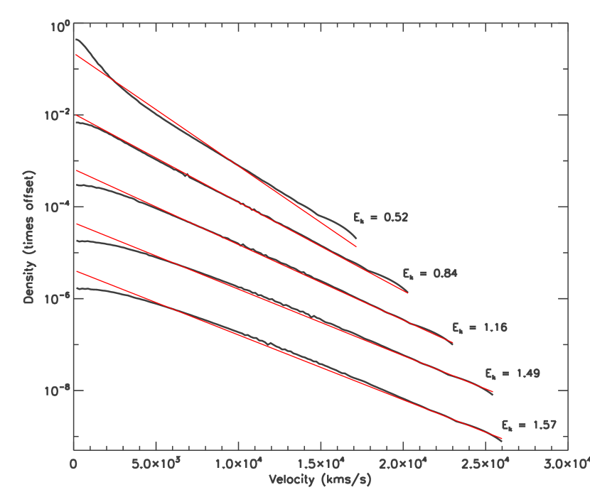
Figure 4.— Logarithm of the density structure of explosion models with different kinetic energy (black lines) compared to the exponential function (Equation 4, red lines). The kinetic energy $E_{K}$ of each model is marked on the figure.

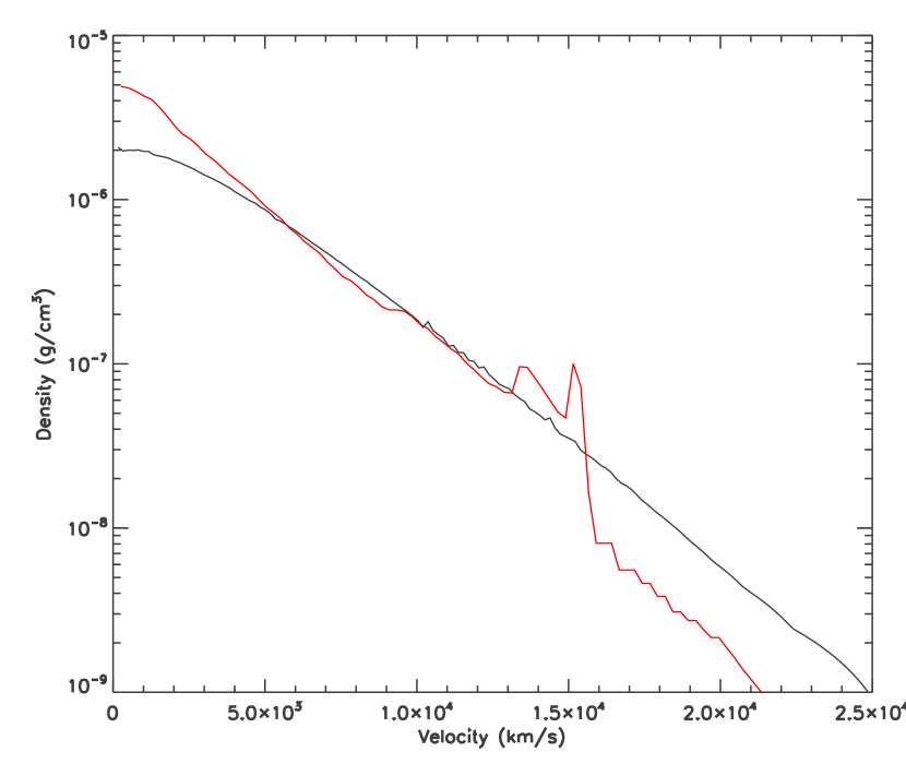
Figure 5.— Logarithm of the density structure at 10000 sec for Model M060303 (black line) compared to that of W7 (red line).

The primary output of the hydrodynamic explosion calculation is the final density structure (e.g., density versus velocity) of the ejecta once it has reached the homologous phase. Interestingly, the final density profiles of all models are well characterized by a simple exponential function which depends only upon the kinetic energy of the explosion

$$\rho(v,t)=\frac{{\mathrm{M}_{\mathrm{ch}}}}{8\pi v_{e}^{3}t^{3}}\exp[-v/v_{e}]$$ (3)

$$\mathrm{where}~{}~{}v_{e}=\sqrt{\frac{E_{k}}{6{\mathrm{M}_{\mathrm{ch}}}}}=2455\biggl{(}\frac{E_{k}}{10^{51}}\biggr{)}^{1/2}~{}\mathrm{km~{}s}^{-1}$$ (4)

Figure 4 shows that this simple analytic formula holds very well for all but the innermost ejecta ($v\lesssim v_{e}$). For the high $E_{K}$ models, the formula overestimates the central densities, while from the low $E_{K}$ models it underestimates them.

The properties of our models can be compared to existing standard SN Ia explosion models. A much studied 1-D model that has been shown to agree with typical observed light curves and spectra is Model W7 of Nomoto, Thielemann, & Yokoi (1984) (see also Thielemann et al., 1986; Iwamoto et al., 1999). In terms of our four composition parameters, the abundances in the final frozen-out Model W7 are ⁵⁶Ni, 0.59 $\mathrm{M}_{\odot}$, stable iron (^54,56Fe, ⁵⁵Mn, ^58,60Ni), 0.26 $\mathrm{M}_{\odot}$, and Si-Ca, 0.27 $\mathrm{M}_{\odot}$. If our simple model for the hydrodynamics is correct and if mixing is not a major issue, this should be a good match for our Model M060303 (which has 0.6, 0.3, and 0.3 $\mathrm{M}_{\odot}$ of ⁵⁶Ni, stable iron and IME respectively).

In Fig. 5, we compare the density profile of Model M060303 to that of W7. The agreement is quite good in the inner layers, although there are discrepancies for velocities $v>13,000$ $\mathrm{km~{}s}^{-1}$. This is the region in which the deflagration burning began to be quenched in W7, which lead to the production of a density spike. This density spike would probably be absent in a multi-dimensional simulation.

In Fig. 6 we compare the light curve and near maximum light spectra ($t_{\mathrm{exp}}$= 18 days) of Model M060303 and W7. Despite the differences in the density profile and approximate representation of the composition in M060303, the overall agreement is reasonably good. The light curves of M060303 are slightly faster than W7, due to the slightly lower densities and greater stable iron group production (see §6.2.2). The maximum light spectra show only minor discrepancies in the lines of calcium and in the ultraviolet reflecting the different mixing employed here and the fact that the Ca abundance in Model M060303 is about twice as large as in W7 (0.024 $\mathrm{M}_{\odot}$vs 0.012 $\mathrm{M}_{\odot}$) and extends to higher velocity.

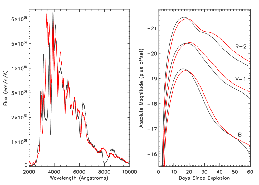
Figure 6.— Demonstration that the simplified Model M060303 (black lines) well reproduces the observable properties of the well-known W7 model (red lines). Left: Comparison of the near maximum light ($t_{\mathrm{exp}}=18$ day) spectra of the two models. Right: Comparison of the $BVR$-band light curves of the two models.

4.3. Comparison to Individual Observations

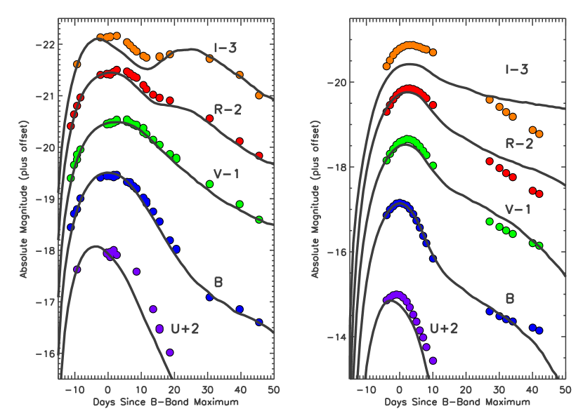
Figure 7.— Right: Comparison of the broadband synthetic light curves of Model M080202 to observations of the bright/broad Type Ia SN 1991T (Lira et al., 1998). Left: Comparison of the broadband synthetic light curves of Model M010309 to observations of the Type Ia SN 1999by, a subluminous SN 1991bg-like event (Garnavich et al., 2004).

Figure 8.— Verification of the Model M070103 against SN Ia observations. Left: Synthetic broadband light curves of the model (solid lines) compared to observations of the normal Type Ia SN 2001el (Krisciunas et al., 2003, filled circles). In order to improve the visual comparison, the observations have been offset by $-0.1$ mag in order to better align them with the model light curves. Right: Synthetic spectra at three different epochs with respect to $B$-band maximum of the model (black lines) compared to observations of the normal Type Ia SN 1994D (red lines).

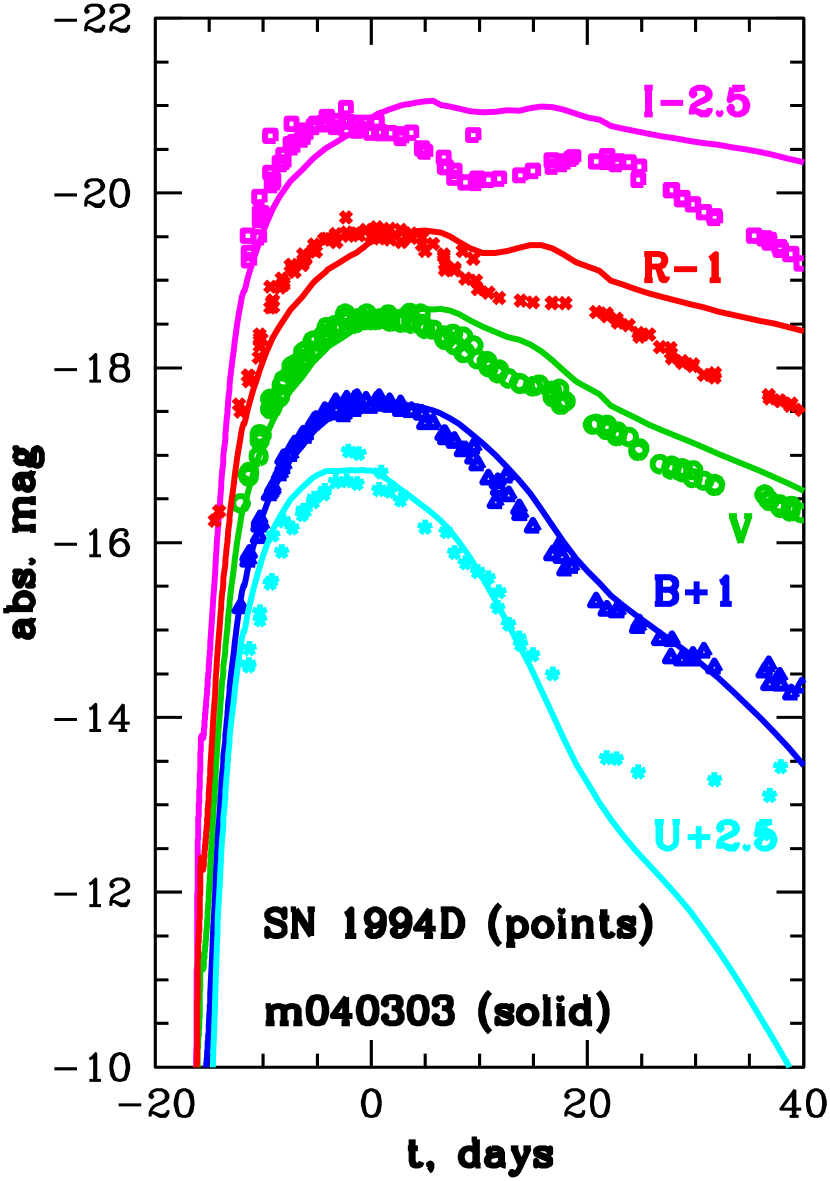
Figure 9.— Comparison of the broadband synthetic light curves of Model M040303, computed by stella (solid lines), to observations of the Type Ia SN 1994D (Richmond et al., 1995; Meikle et al., 1996)

Within our model grid are examples that resemble a broad range of observed SNe Ia, from photometrically normal events like SN 2001el, to bright, broad events like SN 1991T, and faint, narrow ones like SN 1991bg. In Fig. 8, the $UBVRI$ light curves Model M070103 ($M_{\mathrm{Ni}}=0.7~{}{\mathrm{M}_{\odot}}$) are compared with those of the normal Type Ia SN 2001el (Krisciunas et al., 2003). The observed light curves of SN 2001el have been corrected for dust extinction using the estimates $A_{v}=0.57$ and $R_{v}=2.88$, and the distance modulus is taken to be $\mu=31.3$ (Krisciunas et al., 2003; Wang et al., 2003). Generally good agreement between model and observations is found in all bands. The model further reproduces the double-peaked behavior of the I-band light curve, although the secondary maximum is stronger than in the observations.

Figure 7 demonstrates that our models also include examples resembling more extreme SNe Ia events. The left panel of the figure compares the light curves of Model M080101 ($M_{\mathrm{Ni}}=0.8~{}{\mathrm{M}_{\odot}}$) to those of the overly bright SN 1991T (Lira et al., 1998). We adopt the reddening estimate of $A_{v}=0.50.~{}R_{v}=3.1$ from Phillips et al. (1999) and the Cepheid distance measurement of $\mu=30.56$ from Gibson & Stetson (2001), although there is substantial uncertainty in these values. The right panel of the figure compares the light curves of Model M010207 ($M_{\mathrm{Ni}}=0.1~{}{\mathrm{M}_{\odot}}$) to those of the subluminous SN 1991bg-like event SN 1999by. The reddening and distance here are taken to be $A_{v}=0.43,~{}R_{v}=3.1,~{}\mu=30.75$ (Garnavich et al., 2004). Good agreement with observations is found for both examples.

Full time-series of synthetic spectrum calculations are available from the sedona code and Fig. 8 (right panel) compares the Model M070103 spectra at several epochs to observations of the normal Type Ia SNe 1994D (Meikle et al., 1996; Patat et al., 1996). While there are some differences in detail, the model reproduces quite well the essential spectroscopic features and colors over a wide evolution time. The only major discrepancy occurs in the Ca II IR-triplet features, which is too strong in the model. This confirms the adequacy of the transfer calculations to model the spectral and color evolution of SNe Ia over the timescale of interest.

Fig. 9 compares synthetic light curves of Model M040303, computed by stella, to observations of the Type Ia SN 1994D (Richmond et al., 1995; Meikle et al., 1996). The agreement is especially good in $UBV$, and in general it is not worse than for the MPA deflagration models presented by Blinnikov et al. (2006). Comparison with sedona results for the same model in Fig. 3 suggests that the agreement with observations in $R$ and $I$ filters can be improved by extending the line list used in stella for computing expansion opacity.

5. BASIC PHYSICS OF THE WIDTH-LUMINOSITY RELATION

Before turning to the model calculations, it is useful to summarize the basic radiative transfer physics relating to the brightness and decline rate of SN Ia light curves. A more detailed discussion of the transfer effects can be found in a companion paper (Kasen & Woosley, 2006). Because the light curves of SNe Ia are influenced by a number of physical parameters, the behavior of our model light curves can not usually be explained by referencing a single cause, but rather require consideration of a combination of interrelated transfer effects. We attempt to describe the most important effects individually below.

It is well known that the light curves of SNe Ia are powered entirely by the decay of radioactive ${}^{56}\mathrm{Ni}$ (and its daughter ⁵⁶Co) synthesized in the explosion. The mass of ${}^{56}\mathrm{Ni}$ produced ($M_{\mathrm{Ni}}$) is therefore the primary determinate of the peak brightness of the event. On the basis of approximate analytic models, (Arnett, 1982) showed that the bolometric luminosity at peak is roughly equal to the instantaneous rate of radioactive energy deposition

$$L_{p}\sim fM_{\mathrm{Ni}}\exp(-t_{p}/t_{Ni})$$ (5)

where $t_{p}$ is the rise time to peak, $t_{Ni}\approx 8.8$ days is the ${}^{56}\mathrm{Ni}$ decay time and $f$ is the percentage of the gamma-ray decay energy that is trapped at the bolometric peak (typically $f\gtrsim 0.9$).

In SNe Ia, the ejecta remain optically thick for the first several months after explosion. The width of the bolometric light curve is related to the photon diffusion time. The basic diffusion physics can roughly be understood using simple scaling arguments. In a standard random walk, the diffusion time is given by $t_{d}\sim R^{2}/\lambda_{p}c$ where $R$ is the radius, $\lambda_{p}=1/\kappa\rho$ is the photon mean free path, and $\kappa$ is the mean opacity. In homologous expansion $R={\phi_{\mathrm{Ni}}}vt$ where $v$ is the characteristic ejecta velocity, $t$ is the time since explosion, and $\phi_{\mathrm{Ni}}$ is a factor describing the fractional distance between the bulk of ${}^{56}\mathrm{Ni}$ and the ejecta surface, roughly: ${\phi_{\mathrm{Ni}}}\sim(M-M^{c}_{\mathrm{Ni}})/M$ where $M^{c}_{\mathrm{Ni}}$ is the center of mass of the ${}^{56}\mathrm{Ni}$ distribution. Using the scaling relations for the total ejected mass $M\sim\rho v^{3}t^{3}$ and kinetic energy $E_{K}\sim Mv^{2}$, one finds

$$t_{d}\sim{\phi_{\mathrm{Ni}}}\ \kappa^{1/2}M^{3/4}E_{K}^{-1/4},$$ (6)

The important parameters affecting the bolometric diffusion time are thus the total mass $M$, the kinetic energy $E_{K}$, the radial distribution of nickel $\phi_{\mathrm{Ni}}$, and the effective opacity per unit gram, $\kappa$. The last of these is the most complicated, depending upon the composition, density, and thermal state of the ejecta, as well as the velocity shear across the ejecta. In general, $\kappa$ increases with temperature/ionization, thus models with larger $M_{\mathrm{Ni}}$ will typically have slightly longer diffusion times (Khokhlov et al., 1993; Pinto & Eastman, 2001; Höflich et al., 2002; Kasen & Woosley, 2006)

A further factor influencing the bolometric light curve is the rate at which the ejecta become transparent to gamma-rays from radioactive decay. Near maximum light, the densities in a Chandrasekhar-mass model are high enough that nearly all gamma-rays are trapped locally ($f\gtrsim 0.9$). However, by 15 days after maximum densities have dropped such that a substantial percentage of the gamma-rays escape the ejecta without being thermalized. Models in which the bulk of ${}^{56}\mathrm{Ni}$ is located further out in mass coordinates will experience a more rapid transition to gamma-ray transparency and hence possess a generally faster bolometric decline rate.

In addition to the parameters affecting the bolometric decline rate just mentioned, one must also consider the physics affecting the spectroscopic and color evolution of SNe Ia. In Kasen & Woosley (2006), it was shown that the WLR arises primarily from a broadband effect. In particular, the $B$-band light curve decline rate depends sensitively on the rate at which the SN colors shift progressively redwards following maximum light. Dimmer SNe Ia (i.e., those with lower $M_{\mathrm{Ni}}$) exhibit a generally faster color evolution, which is the primary reason for their faster $B$-band decline. Physically, this reflects the faster ionization evolution of dimmer SNe Ia. Following maximum-light, the SN colors are increasingly determined by the development of numerous Fe II and Co II lines that blanket the bluer wavelength bands and, at the same time, increase the emissivity at longer wavelengths. Because dimmer SNe Ia are generally cooler, they experience an earlier onset of Fe III to Fe II recombination in the iron-group rich layers of ejecta. Consequently, Fe II and Co II line blanketing develops more rapidly in dimmer SNe Ia, resulting in a more rapid evolution of the SN spectral energy distribution to the red. This is the principle explanation for their faster $B$-band decline rate.

As a corollary, one realizes that the velocity distribution of iron group elements plays an additional important role in determining the broadband light curves. Models in which iron group elements are concentrated at low velocities are unable to form strong Fe II/Co II line features in the post-maximum epochs, and consequently will exhibit a slower color evolution (and hence $B$-band decline rate) compared to those in which the iron group elements are mixed out to higher velocity.

6. RESULTS

6.1. All Models Combined

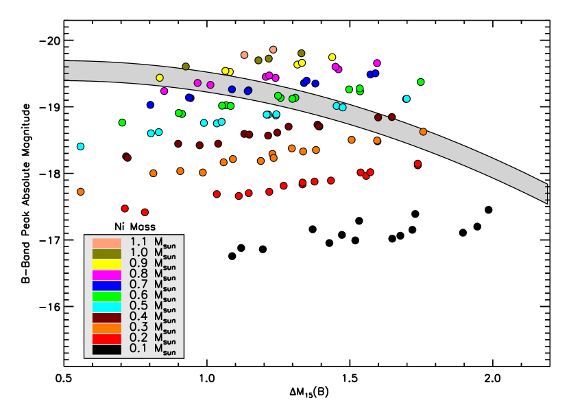
Figure 10.— Relationship between the $B$-band decline rate $\Delta M_{15}(B)$ and peak $B$-band magnitude for the full set of M-series models. The color coding shows the ${}^{56}\mathrm{Ni}$ mass, which varies from $0.1$ to $1.1$ $\mathrm{M}_{\odot}$. The shaded region is the observed width-luminosity relation of Phillips et al. (1999) with a calibration $M_{B}=-19.3$ for $\Delta M_{15}(B)=1.1$ and a dispersion of $\sigma=0.15$ mag. In contrast to the observations, the models occupy a wide region in the plot, indicating a sensitivity of the light curves to parameters other than ${}^{56}\mathrm{Ni}$.The systematic offset of $\sim 0.06$ magnitudes in color between the observations and models suggests that assumed thermalization parameter $\epsilon_{\rm th}=1$, likely overestimates the actual redistribution probability.

Figure 11.— Relationship between the $B$-band decline rate $\Delta M_{15}(B)$ and peak $B$-band magnitude for the full set of M-series models computed by stella. The color coding is the same as in Fig.10.

Figure 12.— Relationship between the maximum light $B$-$V$ color and the peak $B$-band magnitude for the full set of M-series models. The color coding shows the ${}^{56}\mathrm{Ni}$ mass, which varies from $0.1$ to $1.1$ $\mathrm{M}_{\odot}$. The solid line is the observed relation of Phillips et al. (1999), with a calibration $M_{B}=-19.3$ for $\Delta M_{15}(B)=1.1$.

The WLR is often quantified as relation between peak $B$-band magnitude $M_{B}$ and the drop in $B$-band magnitude 15 days after peak $\Delta M_{15}(B)$. Figures 10 and 11 show the WLR for the full set of moderately mixed models calculated with the sedona and stella codes, respectively. The models are color-coded by the mass of ${}^{56}\mathrm{Ni}$ each produces as defined in Fig. 10. Overplotted in both figures, as a shaded band, is the empirical WLR of Phillips et al. (1999), for which an absolute calibration of $M_{B}=-19.3$ mag at $\Delta M_{15}(B)=1.1$ mag and a dispersion of $\sigma=0.15$ mag (Hamuy et al., 1996) have been adopted.

In contrast to the observed behavior, the models span a wide region in the figure. Contrary to popular expectations, the light curve width and luminosity are not both determined by a single parameter, the ⁵⁶Ni produced in the explosion. If this were the case, all models with a given mass of ⁵⁶Ni would collapse to one point on the plot, and that point would be in the gray band.

As the plots confirm, $M_{\mathrm{Ni}}$ is clearly the dominant parameter affecting the SN peak magnitude. For a given $M_{\mathrm{Ni}}$ value, $M_{B}$ varies only by about $\pm 0.25$ mag. The decline rate $\Delta M_{15}(B)$, on the other hand, spans at least a full magnitude for a given $M_{\mathrm{Ni}}$ mass, indicating its sensitivity to additional physical parameters. Given the scaling of the diffusion time (Equation 6), one can anticipate that two very important parameters are the total kinetic energy of the explosion, $E_{K}$, and the radial distribution of ${}^{56}\mathrm{Ni}$, $\phi_{\mathrm{Ni}}$. This is confirmed in the following sections by examining suitable subsets of models.

Careful examination of the figures shows, in fact, that for fixed $M_{\mathrm{Ni}}$, the model light curves actually exhibit an “anti-Phillips relation”, i.e., the brighter supernovae are more narrow. This is not a surprising result, as SNe with shorter diffusion times (i.e., faster light curves) lose a smaller percentage of their internal energy to adiabatic expansion, and thus reach a brighter peak earlier. Equivalently, this can understood as an expression of Arnett’s rule (Equation 5). Models with broader light curves typically have a longer rise time $t_{p}$ and thus, for given $M_{\mathrm{Ni}}$, are dimmer at peak.

Although the models in Figs. 10 and 11 do not reproduce the observed WLR relation, they nonetheless lead to a very important physical insight – the true SN Ia explosion mechanism realizes only a small subset of the theoretically conceivable possibilities, implying a rather tight internal correlation between the relevant physical parameters. This places a strong constraint on theoretical explosion paradigms. Indeed, in the following we use this constraint to deduce some of the properties of the SN Ia ejecta structure.

The large spread seen in Figs. 10 and 11 also suggests that intrinsic SN variation is likely a significant source of intrinsic scatter in the WLR. Because $\Delta M_{15}(B)$ depends upon other parameters than $M_{\mathrm{Ni}}$, any uncorrelated variation of the secondary parameters leads to dispersion in the WLR. Any systematic variation of the parameters with progenitor environment could form a potential basis for evolutionary effects.

Interestingly, if one plots the peak model magnitudes of the entire set vs the $B$-$V$ at maximum instead of $\Delta M_{15}(B)$, a tighter correlation results (Fig. 12). The slope of the model correlation closely resembles that of the observed relation given in Phillips et al. (1999). The models are systematically redder than the observations by $\sim 0.06$ mag, suggesting that our assumed thermalization parameter ($\epsilon_{\rm th}=1$) likely overestimates the true redistribution probability in SNe Ia (§ 3.1). Though it is clear that not all the models shown in Fig. 12 are frequently realized in nature, the smaller dispersion suggests that such color indicators may be less sensitive to intrinsic variation in the supernovae.

6.2. Sources of Dispersion

The large spread in the model WLR of Figs. 10 and 11 indicates that parameters other than $M_{\mathrm{Ni}}$ significantly affect the light curves of SNe Ia. We show below that the most important of these are the total burned mass, $\mathrm{M}_{\mathrm{burn}}$, which determines the $E_{K}$, and the stable iron mass, $M_{\mathrm{Fe}}$, which influences $\phi_{\mathrm{Ni}}$. In addition, the degree of direct ${}^{56}\mathrm{Ni}$ mixing is significant as well. For a given $M_{\mathrm{Ni}}$  these parameters have significant impact on the decline rate $\Delta M_{15}(B)$, and hence may act as sources of dispersion in the WLR. Here the effects of each are quantified using suitable subsets of the models

6.2.1 Effect of the Total Burned Mass

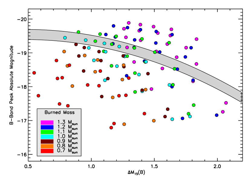
Figure 13.— Same as Fig. 10, but color coded to show the total burned mass of the models. Models with the same total explosion energy, i.e., points of the same color do roughly yield a width-luminosity relation in which “brighter equals broader”. The best agreement is for a burned mass of $1.1\pm 0.1$ $\mathrm{M}_{\odot}$, though the narrower light curves are somewhat fainter than the observations if burned mass is a constant.

Figure 14.— Effect of the total burned mass (and hence kinetic energy) on the $B$-band light curve for a subset of M-series models with constant ${}^{56}\mathrm{Ni}$. The models shown have $M_{\mathrm{Ni}}$= 0.5 $\mathrm{M}_{\odot}$ and $M_{\mathrm{Fe}}$= 0.1 $\mathrm{M}_{\odot}$ and $M_{\mathrm{IME}}$= $[0.1,0.3,0.5,0.7~{}{\mathrm{M}_{\odot}}]$. The left panels shows the $B$-band model light curves, while the right panel shows the corresponding width-luminosity relation (as in Fig. 10). For a constant ${}^{56}\mathrm{Ni}$ mass, models with a greater total burned mass have higher kinetic energy, and hence faster light curves. All else being equal, the full width of the observed region corresponds to a range in burned mass of only 0.2 $\mathrm{M}_{\odot}$.

The models shown in Figs. 10 and 11 span a wide range in the fraction of the original white dwarf which is burned to heavier elements. Because the nuclear energies released in burning carbon and oxygen to iron, ⁵⁶Ni or IME are all about the same, and since the same initial white dwarf is used for all calculations, the total mass burned in the explosion, $\mathrm{M}_{\mathrm{burn}}$, essentially dictates the final kinetic energy, $E_{K}$, of the ejecta. Given the inverse dependence of the diffusion time on $E_{K}$ (Equation 6), a higher value of $\mathrm{M}_{\mathrm{burn}}$ can be expected to lead to a relatively faster bolometric light curve for any given model. In addition, because the velocity of the bulk of ${}^{56}\mathrm{Ni}$ ejected in the explosion increases with $E_{K}$, a higher $\mathrm{M}_{\mathrm{burn}}$ should also lead to a faster evolution of the model colors and gamma-ray transparency, both of which further contribute to a faster $B$-band light curve decline (§ 5).

Figure 13 redisplays the same full model set as in Figs. 10 and 11, but now color coded by the total burned mass. Models with higher $\mathrm{M}_{\mathrm{burn}}$ (high $E_{K}$) generally occupy the faster declining portion of the plot while models with lower $\mathrm{M}_{\mathrm{burn}}$ have overly broad light curves. It is clear from the figure that a large part of the spread in the model WLR is due to the variations in $\mathrm{M}_{\mathrm{burn}}$ among the models. Eliminating both the very high and very low $\mathrm{M}_{\mathrm{burn}}$ points does result in a loose inverse correlation between peak brightness and decline rate (i.e., brighter is general broader), though there is still a large dispersion compared with observations. The best agreement with observations is achieved if common SN Ia burn 1.0 to 1.2 $\mathrm{M}_{\odot}$ of their mass to silicon and heavier elements. Without further modification, models that burn 0.7, 0.8, and 1.3 $\mathrm{M}_{\odot}$ seem to be rare events.

We can further quantify the effect of $\mathrm{M}_{\mathrm{burn}}$ on the light curves by examining a subset of models with fixed $M_{\mathrm{Ni}}=0.5$ $\mathrm{M}_{\odot}$ and $M_{\mathrm{Fe}}=0.1~{}{\mathrm{M}_{\odot}}$, but with $M_{\mathrm{IME}}$ varied from 0.1 to 0.7 $\mathrm{M}_{\odot}$. The total burned mass among these models thus varies from $\mathrm{M}_{\mathrm{burn}}$ = 0.7-1.3 $\mathrm{M}_{\odot}$ corresponding to a variation of $E_{K}$ from 0.68 to 1.43 B. Figure 14 shows that the models obey an anti-Phillips relation. Models with higher $\mathrm{M}_{\mathrm{burn}}$ have shorter rise times and faster declines, and are also brighter at peak. Quantitatively, increasing the amount of burned IME mass by 0.2 $\mathrm{M}_{\odot}$ (a $E_{K}$ increase of 0.25 B) increases $M_{B}$ by 0.1 mag, $\Delta M_{15}(B)$ by 0.2 mag, and decreases the $B$-band rise time by 3 days.

6.2.2 Effect of the Mass of stable iron and Mixing

Figure 15.— Effect of changing the mass of stable iron-group elements ($M_{\mathrm{Fe}}$) on the $B$-band light curve for a subset of M-series models. Same as Fig. 14, expect that here the mass of ${}^{56}\mathrm{Ni}$ and the explosion energy are held constant (${\mathrm{M}_{\mathrm{burn}}}=1.1~{}{\mathrm{M}_{\odot}}$, in all cases), while the amount of stable iron is varied at the expense of IME. Here $M_{\mathrm{Ni}}$= 0.5 $\mathrm{M}_{\odot}$, $M_{\mathrm{Fe}}$= $[0.0,0.1,0.2,0.3~{}{\mathrm{M}_{\odot}}]$ and $M_{\mathrm{IME}}+M_{\mathrm{Fe}}=0.6~{}{\mathrm{M}_{\odot}}$. Models with larger $M_{\mathrm{Fe}}$ have ${}^{56}\mathrm{Ni}$ distributed closer to the surface, and hence faster light curves. A change in $M_{\mathrm{Fe}}$ of only 0.1 $\mathrm{M}_{\odot}$ gives the entire width of the observed band.

Figure 16.— Effect of the degree of “mixing” on the $B$-band light curve. Same as Fig. 14, but for four models all with the same ejected composition, $M_{\mathrm{Ni}}=0.5~{}{\mathrm{M}_{\odot}}$, $M_{\mathrm{Fe}}=0.1~{}{\mathrm{M}_{\odot}}$, $M_{\mathrm{IME}}=0.5~{}{\mathrm{M}_{\odot}}$, but each with different mixing prescriptions. The more heavily mixed models have ${}^{56}\mathrm{Ni}$ distributed closer to the surface and hence faster light curves.

The second important model parameter leading to the dispersion in Figs. 10 and 11 is the mass of stable iron, $M_{\mathrm{Fe}}$. Since it is not a source of radioactive decay energy, and since its opacity is not so different from ${}^{56}\mathrm{Ni}$, the chief effect of $M_{\mathrm{Fe}}$ is to influence the distribution of ${}^{56}\mathrm{Ni}$. For models with larger values of central $M_{\mathrm{Fe}}$, the ${}^{56}\mathrm{Ni}$ center of mass is pushed farther out, thus decreasing the $\phi_{\mathrm{Ni}}$ parameter (this is not necessarily the case for ⁵⁴Fe and ⁵⁸Ni produced in the ${}^{56}\mathrm{Ni}$ zones because of a finite metallicity and neutron excess). This can be expected to lead to faster light curves for three reasons discussed in § 5: (1) based upon Equation 6, the diffusion time to the ejecta surface should be shorter; (2) the occurrence of ${}^{56}\mathrm{Ni}$ at lower densities leads to a lower percentage of gamma-ray trapping in the post-maximum epochs; and (3) the increase in iron group elements at higher velocity layers of ejecta leads to the stronger development of Fe II/Co II features in the post-maximum spectra, contributing to a faster color evolution (and hence $B$-band decline rate).

To demonstrate the important effect of $M_{\mathrm{Fe}}$ in Fig. 15, models were selected with fixed $M_{\mathrm{Ni}}$= 0.5 $\mathrm{M}_{\odot}$ and fixed $\mathrm{M}_{\mathrm{burn}}$= 1.1 $\mathrm{M}_{\odot}$, but with $M_{\mathrm{Fe}}$ varied from 0.0 to 0.3 $\mathrm{M}_{\odot}$. The models also obey an anti-Phillips relation – for given $M_{\mathrm{Ni}}$, models with larger $M_{\mathrm{Fe}}$ have faster light curves. Quantitatively, increasing $M_{\mathrm{Fe}}$ by 0.1 $\mathrm{M}_{\odot}$ increases $M_{B}$ by 0.05 mag, $\Delta M_{15}(B)$ by 0.1 mag, and decreases the $B$-band rise time by 2 days.

These effects of $M_{\mathrm{Fe}}$ on the light curves are not related to the presence of stable iron group elements per se, but to the effect $M_{\mathrm{Fe}}$ has on the distribution of ${}^{56}\mathrm{Ni}$. Essentially the same effect can be demonstrated more directly by varying the degree of mixing in the model. In Fig. 16 we show four models each with the same compositional production ($M_{\mathrm{Ni}}=0.5~{}{\mathrm{M}_{\odot}}$, $M_{\mathrm{Fe}}=0.1~{}{\mathrm{M}_{\odot}}$, $M_{\mathrm{IME}}=0.5~{}{\mathrm{M}_{\odot}}$) but each with different degrees of mixing. The more heavily mixed models have a greater proportion of ${}^{56}\mathrm{Ni}$ in the outer layers of ejecta, and hence faster light curves, for the same three reasons given above.

7. TOWARDS A WORKING MODEL

Having identified the two principal physical parameters that cause dispersion in the model WLR – the explosion energy and the distribution of ${}^{56}\mathrm{Ni}$ in the ejecta, selected subsets of the models are now examined that are in better accordance with the observations. What are the common properties of those “viable” models that fall within the observed WLR in Figs. 10 and 11, and why is the observed scatter so small?

7.1. Constraints from Nucleosynthesis and Nuclear Physics

Figure 17.— Same as Fig. 10, but including only those models which obey the observational constraints of rapid expansion and “reasonable” nucleosynthesis and spectra, ${\mathrm{M}_{\mathrm{burn}}}=1.1\pm 0.1$ $\mathrm{M}_{\odot}$, $M_{\mathrm{IME}}\geq 0.1~{}{\mathrm{M}_{\odot}}$, $M_{\mathrm{Fe}}=0.1-0.3~{}{\mathrm{M}_{\odot}}$.

Figure 18.— Same as Fig. 12, but including only those models which obey the observational constraints of rapid expansion and “reasonable” nucleosynthesis and spectra, ${\mathrm{M}_{\mathrm{burn}}}=1.1\pm 0.1$ $\mathrm{M}_{\odot}$, $M_{\mathrm{IME}}\geq 0.1~{}{\mathrm{M}_{\odot}}$, $M_{\mathrm{Fe}}=0.1-0.3~{}{\mathrm{M}_{\odot}}$. Once again, the solid line is the observed relation of Phillips et al. (1999), with a calibration $M_{B}=-19.3$ for $\Delta M_{15}(B)=1.1$. The systemmatic offset of $\sim 0.06$ magnitudes in color between the observations and models suggests that assumed thermalization parameter $\epsilon_{\rm th}=1$, likely overestimates the actual redistribution probability.

First, one might consider what is “reasonable” from other quarters. Nature does not just select, with equal frequency, any random combination of nuclear products that unbind the star, but must select values consistent with known nuclear physics and, on the average, with the requirements of stellar nucleosynthesis and SN Ia spectroscopy (e.g., the presence of IME in the spectrum). Does the application of these observational constraints serve to increase the agreement of the models with the WLR?

It is not reasonable, for example, that a SN Ia make no stable iron, but only ${}^{56}\mathrm{Ni}$. Ignition in models near the Chandrasekhar mass can only be achieved at densities in excess of about $2.5\times 10^{9}$ g cm^-3 and any burning near that density makes ^54,56Fe and ^58,60Ni, not ${}^{56}\mathrm{Ni}$. Further, if the star has any appreciable metallicity, the excess neutrons will mostly end up in these same stable iron-group isotopes. As Timmes et al. (2003) discuss, all initial CNO will end up at the end of helium burning in the isotope ²²Ne, creating a mass fraction approximately 0.02 (Z/$Z_{\odot}$). Subsequent burning and conservation of neutrons turns this chiefly into ⁵⁴Fe and ⁵⁸Ni with a combined mass fraction $\approx 0.05$ Z/$Z_{\odot}$. For a range of ${}^{56}\mathrm{Ni}$ masses up to 1 $\mathrm{M}_{\odot}$, and metallicities Z = 0 to 3 $Z_{\odot}$, this implies a stable iron mass of 0 to 0.15 $\mathrm{M}_{\odot}$. An additional minimum of 0.1 $\mathrm{M}_{\odot}$ of ⁵⁴Fe is expected from electron capture. This is roughly the amount of burning required to reduce the white dwarf density below the point where electron capture is important; (e.g., Nomoto, Thielemann, & Yokoi, 1984). Thus we expect $M_{\mathrm{Fe}}$ $\scriptscriptstyle>$ $\scriptscriptstyle\sim$ 0.1 $\mathrm{M}_{\odot}$ always.

On the other hand, nucleosynthesis in the Milky Way Galaxy requires that the sum of ⁵⁴Fe and ⁵⁸Ni be approximately 10% by mass that of ⁵⁶Fe. Given that massive stars also make some iron, this might possibly be raised to $\sim$15%, but the iron in Type II supernovae is made in a region of high neutron excess as well. This suggests that Galactic SN Ia do not, on the average, make more than 0.2 $\mathrm{M}_{\odot}$ of stable iron per event. Of course, one does not know the isotopic composition of iron in distant galaxies. It is reasonable, however, that whatever physical constraints operate to limit the amount of electron capture in local SN Ia also function in similar explosions far away. In summary, it seems that the stable iron mass is restricted by nuclear physics and nucleosynthesis to typically 0.1 to 0.3 $\mathrm{M}_{\odot}$ even for metallicities as high as three times solar. This does not mean there cannot occasionally be supernovae with very different characteristics. Nucleosynthesis constraints only operate on the average.

The total mass burned is also limited by observational constraints on the typical expansion speed. The supernovae do not come apart with only a small excess of total energy over the binding energy, or spectral lines would be too narrow and ionization stages too neutral. In terms of light curves, it is already known from Fig. 13 that approximately 1.1 $\mathrm{M}_{\odot}$ needs to burn. This means that the typical model burns most of its mass. That is natural in all detonation models, and also true of strong deflagrations.

Finally, the presence of strong silicon, sulfur and calcium lines in the maximum-light spectrum of SNe Ia implies the production of at least 0.1 $\mathrm{M}_{\odot}$  and probably 0.2 $\mathrm{M}_{\odot}$ of IME for normal events. For these elements, there is no nucleosynthetic upper bound and the spectroscopic limits are not presently highly constraining.

Figure 17 and Figure 18 show the resulting plots of $M_{B}$vs $\Delta M_{15}(B)$ and $M_{B}$ vs $B$-$V$ when these constraints are applied. In particular, we choose those models with ${\mathrm{M}_{\mathrm{burn}}}=1.1\pm 0.1$ $\mathrm{M}_{\odot}$, $0.1\geq M_{\mathrm{Fe}}\leq 0.3$ $\mathrm{M}_{\odot}$and $M_{\mathrm{IME}}\geq 0.1$ $\mathrm{M}_{\odot}$. Unlike Fig. 10, the more restricted models do show a WLR, albeit a noisy one. The scatter in the color-brightness plot is also reduced. Nature apparently realizes this limited set of models more frequently. The WLR exists, not because a single parameter, the ${}^{56}\mathrm{Ni}$ abundance determines both the brightness and decline rate of SN Ia, but because of other physics that constrains the production and distribution of stable iron, ${}^{56}\mathrm{Ni}$, and IME.

The correlation between color and peak magnitude continues to be tight in Fig. 18, though the models are offset to the red about 0.06 magnitudes. This again probably reflects a thermalization efficiency of less than 100% (§ 3.1).

7.2. A Constant Mass of Iron Group Elements

Figure 19.— Left: WLR for a more finely gridded set of the mildly mixed (M-series) of models which obey the constraints ${\mathrm{M}_{\mathrm{burn}}}=1.0-1.1~{}{\mathrm{M}_{\odot}}$, $M_{\mathrm{Fe}}=0.1-0.3$ $\mathrm{M}_{\odot}$, and $M_{\mathrm{IME}}\geq 0.1$ $\mathrm{M}_{\odot}$. The ${}^{56}\mathrm{Ni}$ mass varies from $M_{\mathrm{Ni}}=0.4-0.8$ $\mathrm{M}_{\odot}$, with the same color coding as in Figure 10. Right: Same as left, but including only those models that have total iron group production in the range $M_{\mathrm{Fe}}+M_{\mathrm{Ni}}=0.7-0.9~{}{\mathrm{M}_{\odot}}$.

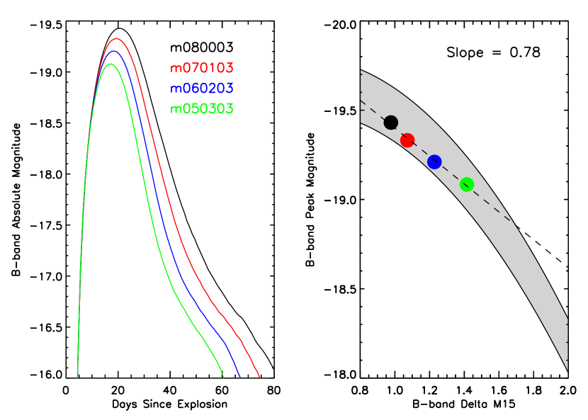
Figure 20.— Effect of varying $M_{\mathrm{Ni}}$ while keeping the total iron group production ($M_{\mathrm{Ni}}+M_{\mathrm{Fe}}$) fixed. The models shown have $M_{\mathrm{Ni}}=[0.5,0.6,0.7,0.8]$ $\mathrm{M}_{\odot}$, $M_{\mathrm{IME}}=0.3$ $\mathrm{M}_{\odot}$, and $M_{\mathrm{Fe}}+M_{\mathrm{Ni}}=0.8$ $\mathrm{M}_{\odot}$. Such a variation might be attributed to a variable amount of electron capture and metallicity in an otherwise standard supernova. However, Model M080003, which has no neutronized iron, is not realistic. The total range of metallicity and electron-capture effects is probably bounded by the red and green points, i.e., about 0.3 magnitudes. The range of metallicity effects alone is less.

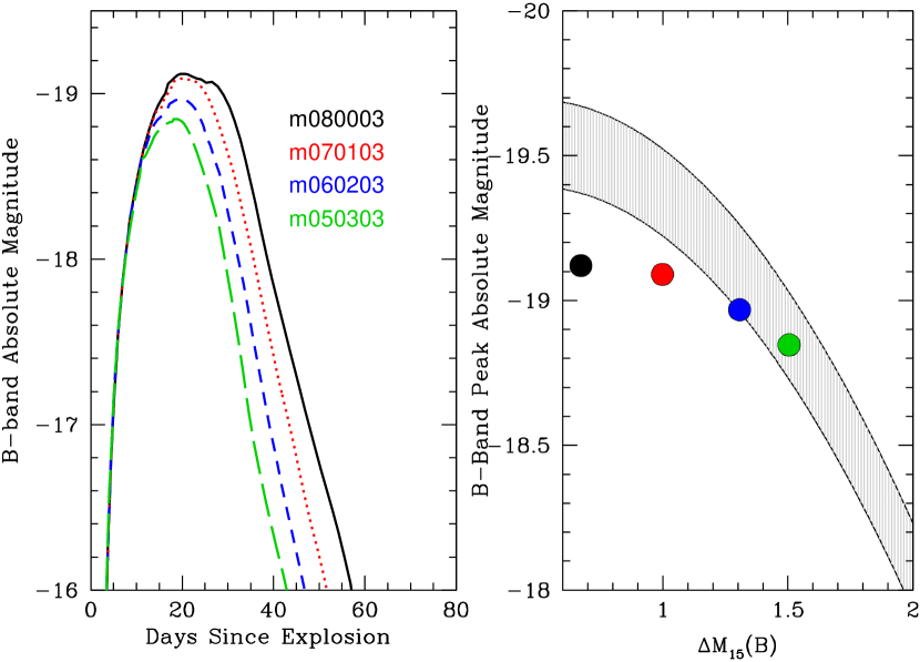
Figure 21.— Same as Fig. 20, but computed with stella. A WLR of the correct sign is also present, though the agreement with observations for these particular models is not as good. For models with a small quantity of initial iron, especially M080003 and M070103, the light curve at early times is fainter in stella because of a deficiency of lines included for Ni and Co (the Fe line list is more nearly complete). See text.

Figure 22.— Effect of varying the abundance of stable iron group throughout the ${}^{56}\mathrm{Ni}$ zone, as might be attributable to variations in progenitor metallicity. The figure shows six models derived from Model M070103, in which the ratio of stable iron to ${}^{56}\mathrm{Ni}$ is varied throughout the ${}^{56}\mathrm{Ni}$ zone from 0 to 25%. All models have, in addition, 0.1 $\mathrm{M}_{\odot}$ of stable iron at the center of the ejecta. The total mass of stable iron thus varies from 0.1 to 0.275 $\mathrm{M}_{\odot}$. The models follow the observed WLR.

The scatter of model points in Fig. 17 is still much greater than observed. To reduce it further, more stringent restrictions must be applied. In order to further populate the allowed band, addition M-series models were constructed obeying the following constraints: ${\mathrm{M}_{\mathrm{burn}}}=1.0-1.1~{}{\mathrm{M}_{\odot}}$, $M_{\mathrm{Fe}}=0.1-0.3$ $\mathrm{M}_{\odot}$ and $M_{\mathrm{IME}}\geq 0.1$ $\mathrm{M}_{\odot}$. A smaller range of ${}^{56}\mathrm{Ni}$ masses were also explored $M_{\mathrm{Ni}}=0.4-0.8$ $\mathrm{M}_{\odot}$. Figure 19 (left panel) shows the width-luminosity relation for this set of models. The scatter is reduced compared to the full plot, but is still larger than the observed.

A second cut of these models is then made assuming that the total mass of iron group elements, as well as the total burned mass, must also lie within a restricted range. Figure 19 (right panel) shows only those models in which $M_{\mathrm{Fe}}+M_{\mathrm{Ni}}=0.7-0.9~{}{\mathrm{M}_{\odot}}$, which are seen to be the models that fall within the observed WLR.

The necessity of having iron group elements in the region 0.7-0.9 $\mathrm{M}_{\odot}$ follows from the spectroscopic and color evolution effect discussed in Kasen & Woosley (2006). The $B$-band decline rate is largely determined by the rate at which Fe II/Co II line blanketing develops in the post-maximum spectra. In order for this line blanketing to develop, there must be a high abundance of iron group elements out to layers $v\approx 8000~{}\mathrm{km~{}s}^{-1}$ which corresponds to mass coordinate $m=0.8~{}{\mathrm{M}_{\odot}}$. This can also be achieved by mixing.

It is not unreasonable that the explosion produce a nearly constant mass of iron group elements. The isotopic composition may vary because of ignition density and metallicity, but all matter that burns with a temperature over $\sim 5\times 10^{9}$ K will be iron-peak isotopes of some variety. Apparently, not only do common SN Ia burn a nearly constant fraction of their total mass, but a nearly constant fraction of that achieves nuclear statistical equilibrium. Delayed detonation at a nearly constant density (after a nearly constant amount of mass has been burned) might be one way, but not the only way of achieving that requirement.

7.3. Variable Electron Capture and Metallicity

The results of the last section suggest that SNe Ia models in which both the total iron group production and the total mass burned are constants of the explosion are in better accord with the observed WLR. In such a scenario, the amount of $M_{\mathrm{Ni}}$ is varied at the expense of stable iron group elements such as ${}^{54}\mathrm{Fe}$ and ${}^{58}\mathrm{Ni}$. There are two ways in which this may come about.

First, stable iron group elements are produced at the center of the ejecta from electron capture (embodied in our $M_{\mathrm{Fe}}$ parameter). If the central density of the white dwarf is higher, electron capture will be enhanced and the ratio of $M_{\mathrm{Fe}}$ to $M_{\mathrm{Ni}}$ will increase. Such variations in ignition density might reflect variations in accretion rate in binaries with different separation, masses, metallicity, etc. A second mechanism that will vary the ratio $M_{\mathrm{Ni}}$ to $M_{\mathrm{Fe}}$ is the progenitor metallicity, which determines the relative abundance of ${}^{56}\mathrm{Ni}$ to ${}^{54}\mathrm{Fe}$ when burning to nuclear statistical equilibrium (Timmes et al., 2003).

These two effects are difficult to separate in the model, though there are observational constraints on the effect of metallicity (Gallagher et al., 2005). In the models, electron capture produces a more centrally concentrated distribution of stable iron, while increased metallicity makes the iron in the same place as the ${}^{56}\mathrm{Ni}$. But the effect on the light curve of increased electron capture plus extensive mixing may be indistinguishable from that of increased metallicity (though see Höflich et al., 1998, mixing all the way to the surface has observational diagnostics. We have in mind mixing that does not extend to the outer layers.).

These two effects are demonstrated in Figs. 20, 21, and 22. Figure 20 shows M-series models in which $M_{\mathrm{Ni}}$ is varied from $0.5$ to $0.8$ $\mathrm{M}_{\odot}$, but $M_{\mathrm{Fe}}+M_{\mathrm{Ni}}=0.8~{}{\mathrm{M}_{\odot}}$, and $M_{\mathrm{IME}}=0.1~{}{\mathrm{M}_{\odot}}$ are both held constant. These models, in which the stable iron remains concentrated at the ejecta center (as expected from electron capture) are in reasonably good agreement with the observed WLR.

Even better agreement is found if the stable iron is mixed throughout the ${}^{56}\mathrm{Ni}$ zone, as expected from variations in metallicity. Figure 22 shows a set of models derived from M070103 in which a constant ratio of ${}^{54}\mathrm{Fe}$ to ${}^{56}\mathrm{Ni}$ is varied from 0 to 25% throughout the ${}^{56}\mathrm{Ni}$ zone. All models have, in addition, 0.1 $\mathrm{M}_{\odot}$ of stable iron located at the ejecta center. The total stable iron mass in these models thus varies from 0.1 to 0.275 $\mathrm{M}_{\odot}$. The models fall very nicely along the observed WLR.

Thus variations in either (or, more likely, both) the progenitor metallicity and the degree of electron capture can be a significant source of the observed luminosity variations in SNe Ia. However, it appears that this effect has a limited range. Varying the metallicity from 0 to 3 times solar only leads to variations of 15% in $M_{\mathrm{Ni}}$. Larger values of metallicity may be unreasonable, and a floor, $\sim 0.1$ $\mathrm{M}_{\odot}$, on the lowest ⁵⁴Fe abundance is set by electron capture (e.g., Nomoto, Thielemann, & Yokoi, 1984). Less than 0.3 magnitudes of the observed peak magnitudes, and perhaps 0.4 magnitudes in decline rate can be explained this way (see also Höflich et al., 1998). This is roughly one-third of the observed spread in peak magnitude for common SN Ia, and is consistent with the observational limits of Gallagher et al. (2005) that metallicity is not the major cause of the width-luminosity relation, or of the preponderance of bright SN Ia in late galaxies (Hamuy et al., 1996). This is especially true, given that part of the spread in Figs.  20 and 22 is due to electron capture during the explosion.

Figure 21 presents the same series of models as Fig. 20, but computed with stella. Reasonably good agreement persists for models that keep both the total iron group production ($M_{\mathrm{Ni}}+M_{\mathrm{Fe}}$) and IME production fixed, though the agreement is less good for brighter, broader supernovae because these models have no or little Fe in the beginning. Although stella has $\sim 10^{5}$ lines of Fe in the opacity, the line list is probably too poor for Ni and Co. Lower opacity means lower emission according to Kirchhoff’s law (which is applicable here when the line opacity is treated as an absorptive one). This makes the brightest models underluminous.

We note that our results in this section differ from the conclusions of Mazzali & Podsiadlowski (2006), who also studied the effect of varying the ratio of stable iron group species to ${}^{56}\mathrm{Ni}$ in SN Ia models. We find that varying this ratio leads to models in general accord with the WLR, whereas Mazzali & Podsiadlowski (2006) find that the variation creates dispersion from it. They therefore identify the ratio as a possible “second parameter” in the WLR. The different conclusions likely stem from the different approaches to the radiative transfer problem. Mazzali & Podsiadlowski (2006) use monochromatic LC calculations and a simplified form of the mean opacity which depends only on the iron group abundance and time. These calculations therefore do not directly capture the critical dependence of the model spectral/color evolution on the ejecta temperature and ionization state. Mazzali & Podsiadlowski (2006) do attempt to quantify the color effects using static synthetic spectra at select epochs. These spectral calculations, however, may be limited by the adoption of an extended inner boundary surface which emits blackbody radiation. In this case, the continuum formation is treated only approximately, and the radius of the inner boundary surface becomes an important free parameter of the calculation.

7.4. Constant $M_{\mathrm{Ni}}+M_{\mathrm{IME}}$

Figure 23.— Effect of varying $M_{\mathrm{Ni}}$ at the expense of IME in moderately mixed models (Fig. 1). The parameters are similar to Fig. 14, except that the mass of stable iron is held fixed while the mass of IME varies: $M_{\mathrm{Ni}}=[0.4,0.5,0.6,0.7,0.8,0.9]$ $\mathrm{M}_{\odot}$, $M_{\mathrm{Fe}}=0.1~{}{\mathrm{M}_{\odot}}$, and $M_{\mathrm{IME}}+M_{\mathrm{Ni}}+M_{\mathrm{Fe}}=1.1~{}{\mathrm{M}_{\odot}}$. The $B$-band peak magnitude declines even faster with decreasing $\Delta M_{15}(B)$ than the observations show. This is because moderately mixed models with large masses of IME and low ${}^{56}\mathrm{Ni}$ have their ${}^{56}\mathrm{Ni}$ more centrally concentrated and thus decline more slowly. Better results are obtained with more mixing (Fig,25).

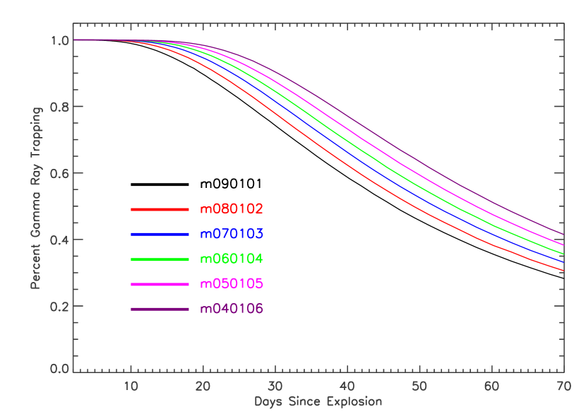
Figure 24.— Percentage of trapping of gamma-rays from radioactive decay as a function of time for the models of Fig. 23 in which $M_{\mathrm{Ni}}$ was varied. Models with lower $M_{\mathrm{Ni}}$ have ${}^{56}\mathrm{Ni}$ concentrated closer to the ejecta center, and hence more efficient gamma-ray trapping in the post-maximum epochs.

Might the good agreement found in the last section persist if ${}^{56}\mathrm{Ni}$ is varied at the expense, not of $M_{\mathrm{Fe}}$, but of IME? The models considered here have fixed $M_{\mathrm{Fe}}$= 0.1 $\mathrm{M}_{\odot}$ and $M_{\mathrm{Ni}}$ varied from 0.4 $\mathrm{M}_{\odot}$ to 0.9 $\mathrm{M}_{\odot}$ at the expense of IME. The procedure is similar to that employed by Pinto & Eastman (2001), but not identical because of issues of mixing and, to a lesser extent, composition and explosion energy. The total iron group production here ($M_{\mathrm{Fe}}$ + $M_{\mathrm{Ni}}$) varied from 0.5 to 1.0 $\mathrm{M}_{\odot}$ while the burned mass was held fixed at $\mathrm{M}_{\mathrm{burn}}$= 1.1 $\mathrm{M}_{\odot}$.

Figure 23 shows that the slope of the WLR for this model set is steeper than observed. The slight positive correlation between $M_{B}$ and $\Delta M_{15}(B)$ is due to the dependence of the spectroscopic/color evolution on $M_{\mathrm{Ni}}$, as discussed in Kasen & Woosley (2006) and § 5 above. However, three other effects act counter to this in the moderately mixed models:

First, in the low $M_{\mathrm{Ni}}$ models, the distribution of ${}^{56}\mathrm{Ni}$ is concentrated closer to the ejecta center. This leads to an increased effectiveness in the trapping of gamma-rays from radioactive decay, as shown in Fig. 24. Near maximum light ($t_{\mathrm{exp}}\approx 20$ days) the differences in gamma-ray trapping among the models are minor, but by day +15 ($t_{\mathrm{exp}}\approx 35$ days) trapping in the $M_{\mathrm{Ni}}$= 0.3 $\mathrm{M}_{\odot}$ model is nearly 40% greater than that in the $M_{\mathrm{Ni}}$= 0.9 $\mathrm{M}_{\odot}$ model. This extra trapping slows the decline rate in the lower $M_{\mathrm{Ni}}$ models.

Second, again because ${}^{56}\mathrm{Ni}$ is more highly concentrated towards the center, the optical depth (and hence diffusion time) to the ejecta surface is significantly larger in the low $M_{\mathrm{Ni}}$ models (see Eq. 6). This further tends to slow the decline rate of these models.

Finally, as mentioned several times already, the $B$-band decline rate is determined largely by color evolution controlled by the development of Fe II and Co II lines. In the low $M_{\mathrm{Ni}}$ models, the iron-group elements extend to only very low velocities. For example in the $M_{\mathrm{Ni}}=0.3$ $\mathrm{M}_{\odot}$ model, the edge of the ${}^{56}\mathrm{Ni}$ zone is at 5000 $\mathrm{km~{}s}^{-1}$ compared to 8500 $\mathrm{km~{}s}^{-1}$ for the $M_{\mathrm{Ni}}$= 0.7 $\mathrm{M}_{\odot}$ model. This inhibits the development of strong Fe II/Co II line blanketing in the low $M_{\mathrm{Ni}}$ models, and hence slows the decline rate of these models.

The very steep WLR seen in Fig. 23 reflects the fact that these three effects act counter to and nearly cancel the spectroscopic, color-evolution effect. Thus, in this particular set of calculations, we find that simply varying the ${}^{56}\mathrm{Ni}$ mass at the expense of IME in a well stratified medium does not give a WLR relation with the correct slope. Either this represents a failure of the assumptions underlying the radiative transfer calculations, or (as we discuss presently) at least a moderate degree of mixing of the zones appears necessary.

7.5. Centrally Concentrated Mixing

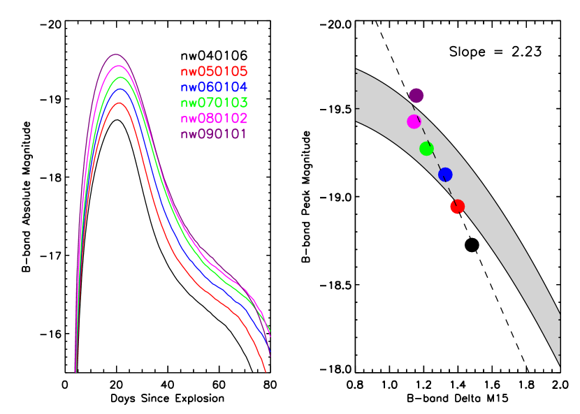
Figure 25.— Effect of varying $M_{\mathrm{Ni}}$ at the expense of IME, but in explosions in which the inner 0.8 $\mathrm{M}_{\odot}$ has been more thoroughly mixed (the “MC” Model in Fig.1). Unlike the stratified M-series models in Fig. 23, the MC-models better reproduce the observed WLR.

Figure 26.— Left: WLR relation for the entire set of mixed core (MC-series) models. These models are characterized by heavy mixing below $m=0.8~{}{\mathrm{M}_{\odot}}$. As in Figure 19, they obey the constraints ${\mathrm{M}_{\mathrm{burn}}}=1.0-1.1~{}{\mathrm{M}_{\odot}}$, $M_{\mathrm{Fe}}=0.1-0.3$ $\mathrm{M}_{\odot}$, and $M_{\mathrm{IME}}\geq 0.1$ $\mathrm{M}_{\odot}$. The ${}^{56}\mathrm{Ni}$ mass varies from $M_{\mathrm{Ni}}=0.4-0.8$ $\mathrm{M}_{\odot}$, with the same color coding as in Figure 10. Right: Same as left, but including only those models that have total iron group production between $M_{\mathrm{Fe}}+M_{\mathrm{Ni}}=0.7-0.9~{}{\mathrm{M}_{\odot}}$.

The models in § 7.4 failed to reproduce the observed WLR because the distribution of iron group elements was more centrally concentrated for the low $M_{\mathrm{Ni}}$ models. This can be rectified if the the inner regions of ejecta are heavily mixed, thus equalizing the distribution (but not quantity) of ${}^{56}\mathrm{Ni}$ among all models. Such mixing could, for example, reflect the maximum extent of the deflagration region in a delayed detonation scenario. The outer part, having been burned by a blast wave, would be less heterogeneous. If the density were low enough, that part would be predominantly IME.

Observationally, the absence of significant high velocity iron in the spectrum suggests that vigorous mixing was restricted to regions  $\scriptscriptstyle<$ $\scriptscriptstyle\sim$0.8 $\mathrm{M}_{\odot}$ (Branch et al., 2005) . Transitions to detonation, if they happen, are believed to occur when the burning enters the “distributed regime” at densities $\sim 1-3\times 10^{7}$ g cm^-3 (Niemeyer & Woosley, 1997). Depending upon the detailed flame model and especially how the burning is ignited, such densities are reached when the flame has moved through $\sim$1 $\mathrm{M}_{\odot}$ (e.g., Nomoto, Thielemann, & Yokoi, 1984). This motivates the studies of models where the mixing has not been uniform, but is concentrated in approximately the inner 0.8 $\mathrm{M}_{\odot}$ of the star where it was assumed to be severe. The MC-series of models was prepared for a restricted range of burned mass, 1.0 and 1.1 $\mathrm{M}_{\odot}$; ${}^{56}\mathrm{Ni}$ masses, 0.4 to 0.9 $\mathrm{M}_{\odot}$  and stable iron masses, 0 - 0.3 $\mathrm{M}_{\odot}$ and a finer sampling of the intervals was also used. These models had the same final elemental yields and explosion energies as the corresponding models in the standard “M” series, but the composition was distributed in a different way. These are called the “MC” (for “mixed core”) models. Figure 1 shows an example that should be compared with the corresponding “M” model.

In Fig. 25 we show the equivalent of the models in Fig. 23 but for the MC series. The mixing of the inner layers leads to an increased agreement with the observed WLR. Meanwhile, Fig. 26 (left panel) shows the full set of MC-series models. Compared to the equivalent set of M-series models (Fig. 19, left panel) the mixing serves to significantly reduce the scatter and improve the agreement with the observed WLR. A more restrictive set of the MC models in which Fe + ${}^{56}\mathrm{Ni}$ = 0.7 to 0.9 $\mathrm{M}_{\odot}$ fits the WLR even better (Fig. 26, right panel).

This final plot shows that it is possible to define a well defined, physically motivated cut of the model templates that does replicate the observed WLR. The chief requisites are: 1) a nearly constant explosion energy (and burned mass) around 1.0 - 1.2 $\mathrm{M}_{\odot}$; 2) ${}^{56}\mathrm{Ni}$ varied at the expense of either stable iron or IME, but sufficiently well mixed in the inner 0.8 $\mathrm{M}_{\odot}$ that its distribution in velocity space does not vary greatly, even when the composition is changed; and 3) a nearly constant iron plus ${}^{56}\mathrm{Ni}$ mass around $0.8\pm 0.1$ $\mathrm{M}_{\odot}$. The resulting WLR is still quite broad though, filling the observed band with no excess left for observational errors and systematics, and there is no a priori reason why the explosions must always be so constrained.

8. CONCLUSIONS

The multi-band photometry (and, in some cases, the spectra) of a large set of Type Ia supernova models have been studied using two approaches to the radiation transport problem. These models were constructed in a simple fashion (§ 2.1) that allowed complete control over the major parameters affecting the outcome - the explosion energy and the masses of ${}^{56}\mathrm{Ni}$, stable iron, and IME produced. The models were exploded by depositing, uniformly, an amount of energy corresponding to the change in composition in a standard white dwarf model. All sensitivity to the uncertain physics of the actual burning was thus absorbed into the three model parameters, plus some prescription for mixing. Comparison of the light curves and spectra of sample models with those of more complicated models and to observations of SN Ia gave good agreement.

Using these models, which consisted essentially of every explosion one could produce starting from a 1.38 $\mathrm{M}_{\odot}$ carbon-oxygen white dwarf, the necessary conditions were determined for reproducing the observed relation between decline rate and peak magnitude (both in the $B$-band). The physical parameters leading to intrinsic dispersion in that relation were also identified and quantified. The relation between peak magnitude and color at peak magnitude was studied as well, and found to be more robust to parameter variation.

The set of all explosions with positive kinetic energy did not give a WLR. Instead a large range of decline rates, quite inconsistent with observations, was found for SN Ia with the same mass of ${}^{56}\mathrm{Ni}$. If SN Ia light curves are a single parameter family, that parameter cannot be as simple as just the mass of ${}^{56}\mathrm{Ni}$. Other possible cuts of the model set were thus considered based upon total kinetic energy (or mass burned), and various restrictions on the final composition and mixing.

In order to satisfy the WLR, the ejecta structures of SNe Ia must obey certain constraints. First, all SNe Ia must have a common total mass burned (and hence kinetic energy). In the present calculations, good agreement with observations was found if that common burned mass was $1.1\pm 0.1$ $\mathrm{M}_{\odot}$ and the kinetic energy at infinity was $1.2\pm 0.2\times 10^{51}$ erg. Second, the radial distribution of iron group elements (including ${}^{56}\mathrm{Ni}$) in the ejecta must be fairly uniform among all SNe Ia. We found the best agreement with the observed WLR among those models where the distribution of iron group elements extended from near the center of the ejecta to $\sim$0.8 $\mathrm{M}_{\odot}$. For example, one can consider the subset of models in which the total mass of iron-group elements is nearly constant at $\sim 0.8\pm 0.1$ $\mathrm{M}_{\odot}$, with variations in $M_{\mathrm{Ni}}$ arising from difference in the ratio of ${}^{56}\mathrm{Ni}$ to stable iron group species produced in the explosion. Differences in this ratio are indeed predicted to arise from metallicity and electron-capture effects, although it is not clear that the entire range of SN Ia luminosities can be so explained given the constraints provided by the underlying explosion physics and Galactic nucleosynthetic measurements. Various arguments lead to the conclusion that the mass of stable iron (mostly ^54,56Fe and ^58,60Ni) is generally restricted to the range 0.1 to 0.3 $\mathrm{M}_{\odot}$ with about half of that range due to metallicity effects. Alternatively, one could vary the amount of ${}^{56}\mathrm{Ni}$ at the expense of IME. In this case, good agreement with the observed WLR is found as long as the inner layers of ejecta ($\lesssim 0.8$ $\mathrm{M}_{\odot}$) are fairly well mixed. In the present calculations, well-stratified ejecta structures do not reproduce the observed slope of the WLR, as the lower $M_{\mathrm{Ni}}$ models have ${}^{56}\mathrm{Ni}$ concentrated relatively closer to the ejecta center, which tends to slow their light curve decline rate. To populate the entire observed span of the WLR, especially at faint luminosities, the mass of these IME is quite large in some instances, arguing for a delayed detonation.

The present calculations adopted an LTE approximation for both the level populations and the line source functions (i.e., the thermalization parameter, $\epsilon_{\rm th}$ = 1). Although a common approach in many previous transfer studies, this (and other simplifying approximations adopted) can be expected to lead to errors in the model observables on the order of 0.1 to 0.3 mag. The relative differences between models, however, may be known more accurately, and so the general trends obeyed by sets of models and the level of dispersion in such trends may be considered more robust. For example, our choice ${\epsilon_{\rm th}}=1$ overestimates the true redistribution probabilities and leads to maximum light colors that are too red by $\sim 0.06$ mag relative to the observations in the color-peak-magnitude plot of, e.g., Fig. 18. Nevertheless, the clustering of the points in this plot is quite tight and the slope is correct. The possible refined calibration of the radiative transfer calculations and its impact on the study of the WLR will be explored further in a subsequent paper.

Given the large dispersion found, even in selected subsets of our models (e.g., Fig. 17), the narrow spread in the observed relation between $M_{B}$ and $\Delta M_{15}(B)$ is surprising. No single physical parameter yields it, unless several other parameters are highly constrained. Part of that spread can be reduced by a judicious choice of mixing and a tight constraint on the mass burned (Fig. 26). Even so, it is difficult to avoid the conclusion that a major fraction of the observed scatter of the WLR, $\lower 0.43057pt\hbox{\hbox to0.0pt{\raise 2.58334pt\hbox{\hskip 1.29167pt{{$\scriptscriptstyle>$}}}\hss} \kern-1.72218pt{{$\scriptscriptstyle\sim$}}}0.1$ mag, reflects intrinsic physical diversity, and not observational effects. This conclusion has important implications as one plans for future studies using SN Ia as calibrated standard candles to ever higher precision. Given the dispersion expected from the models themselves, a larger sample of supernovae will have to be studied to get a strong signal to noise ratio for cosmological effects.

A primary benefit of the approach adopted in this paper is the ability to construct an expansive grid of SNe Ia explosion models without restricting ourselves to any specific theoretical explosion paradigm. Such a large and general database of model light curves and spectra nicely compliments the large sample of SNe Ia data sets currently being acquired by ongoing observational programs. A direct comparison of the models to individual observations would be useful in interpreting the physical properties of any given SN Ia event. In addition, the model grid should be helpful in developing refined techniques for calibrating the luminosities of SNe Ia so as to limit and reduce intrinsic sources of dispersion or evolution. For example, our studies suggest that an improved strategy might be spectroscopic template fitting in which as much data as possible from each individual SN Ia is compared to a template of model spectra and colors. The models employed could be the ones computed here or some derivative of that set.

References

- Arnett (1982) Arnett, W. D. 1982, ApJ, 253, 785
- Bessell (1990) Bessell, M. S. 1990, PASP, 102, 1181
- Blinnikov et al. (1998) Blinnikov, S. I., Eastman, R., Bartunov, O. S., Popolitov, V. A., & Woosley, S. E. 1998, ApJ, 496, 454
- Blinnikov & Sorokina (2000) Blinnikov, S. I., & Sorokina, E. I. 2000, A&A, 356, L30
- Blinnikov et al. (2003) Blinnikov, S., Chugai, N., Lundqvist, P., Nadyozhin, D., Woosley, S., & Sorokina, E. 2003, From Twilight to Highlight: The Physics of Supernovae, 23
- Blinnikov et al. (2006) Blinnikov, S.I., Röpke, F. K., Sorokina, E.I., Gieseler, M., Reinecke, M., Travaglio, C., Hillebrandt, W., and Stritzinger, M. 2006, A&A, 453, 229
- Branch et al. (2005) Branch, D., Baron, E., Hall, N., Melakayil, M., & Parrent, J. 2005, PASP, 117, 545
- Chugai et al. (2004) Chugai, N. N., et al. 2004, MNRAS, 352, 1213
- Eastman & Pinto (1993) Eastman, R. G., & Pinto, P. A. 1993, ApJ, 412, 731
- Gallagher et al. (2005) Gallagher, J. S., Garnavich, P. M., Berlind, P., Challis, P., Jha, S., & Kirshner, R. P. 2005, ApJ, 634, 210
- Garnavich et al. (2004) Garnavich, P. M. et al. 2004, ApJ, 613, 1120
- Gibson & Stetson (2001) Gibson, B. K., & Stetson, P. B. 2001, ApJ, 547, L103
- Hamuy et al. (1996) Hamuy, M., Phillips, M. M., Suntzeff, N. B., Schommer, R. A., Maza, J., & Aviles, R. 1996, AJ, 112, 2391
- Hillebrandt & Niemeyer (1999) Hillebrandt, W., & Niemeyer J. 2000, ARAA, 38, 191b
- Höflich (1995) Höflich, P. 1995, ApJ, 443, 89
- Höflich et al. (1996) Höflich, P., Khokhlov, A., Wheeler, J. C., Phillips, M. M., Suntzeff, N. B., & Hamuy, M. 1996, ApJ, 472, L81
- Höflich et al. (1998) Höflich, P., Wheeler, J. C., & Thielemann, F. K. 1998, ApJ, 495, 617
- Höflich et al. (2002) Höflich, P., Gerardy, C. L., Fesen, R. A., & Sakai, S. 2002, ApJ, 568, 791
- Iwamoto et al. (1999) Iwamoto, K., Brachwitz, F., Nomoto, K., Kishimoto, N., Umeda, H., Hix, W. R., & Thielemann, F.-K. 1999, ApJS, 125, 439
- Kasen (2006) Kasen, D. 2006, Secondary Maximum in the Near-Infrared Light curves of Type Ia Supernovae, ApJ, in press, astro-ph/0606449
- Kasen et al. (2006) Kasen, D., Thomas, R.C., Nugent, P. 2006, Time Dependent Monte Carlo Radiative Transfer Calculations For 3-Dimensional Supernova Spectra, Light curves, and Polarization, ApJ, in press, astro-ph/0606111
- Kasen & Woosley (2006) Kasen, D., & Woosley, S. E. 2006, ApJ, submitted, astro-ph/0609540
- Khokhlov et al. (1993) Khokhlov, A., Mueller, E., & Hoeflich, P. 1993, A&A, 270, 223
- Krisciunas et al. (2003) Krisciunas, K. et al. 2003, AJ, 125, 166
- Kurucz (1994) Kurucz, R. L., 1994, CD-ROM 1, Atomic Data for Opacity Calculations (Cambridge; SAO)
- Lira et al. (1998) Lira, P. et al. 1998, AJ, 115, 234
- Lodders (2003) Lodders, K. 2003, ApJ, 591, 1220
- Lucy (2005) Lucy, L. B. 2005, A&A, 429, 19
- Mazzali et al. (2001) Mazzali, P. A., Nomoto, K., Cappellaro, E., Nakamura, T., Umeda, H., & Iwamoto, K. 2001, ApJ, 547, 988
- Mazzali & Podsiadlowski (2006) Mazzali, P. A., & Podsiadlowski, P. 2006, MNRAS, 369, L19
- Meikle et al. (1996) Meikle, W. P. S., Cumming R. J., Geballe T. R., et al. 1996, MNRAS, 281, 263
- Niemeyer & Woosley (1997) Niemeyer, J. C., & Woosley, S. E. 1997, ApJ, 475, 740
- Nomoto, Thielemann, & Yokoi (1984) Nomoto, K., Thielemann, F.-K., & Yokoi, K. 1984, ApJ, 286, 644
- Patat et al. (1996) Patat, F. et al. 1996, MNRAS, 278, 111
- Perlmutter et al. (1999) Perlmutter, S., et al. 1999, ApJ, 517, 565
- Phillips (1993) Phillips, M. M. 1993, ApJ, 413, L105
- Phillips et al. (1999) Phillips, M. M., Lira, P., Suntzeff, N. B., Schommer, R. A., Hamuy, M., & Maza, J. 1999, AJ, 118, 1766
- Phillips (2005) Phillips, M. M. 2005, ASP Conf. Ser. 342: 1604-2004: Supernovae as Cosmological Lighthouses, 342, 211
- Pinto & Eastman (2000) Pinto, P. A., & Eastman, R. G. 2000, ApJ, 530, 744
- Pinto & Eastman (2001) Pinto, P. A., & Eastman, R. G. 2001, New Astronomy, 6, 307
- Plewa et al. (2004) Plewa, T., Calder, A. C., & Lamb, D. Q. 2004, ApJ, 612, L37
- Pskovskii (1977) Pskovskii, I. P. 1977, Soviet Astronomy, 21, 675
- Richmond et al. (1995) Richmond, M. W., Treffers, R. R., Filippenko, A. V., et al. 1995, AJ, 109, 2121
- Riess et al. (1998) Riess, A. G., et al. 1998, AJ, 116, 1009
- Röpke, Woosley, & Hillebrandt (2006) Röpke, F., Woosley, S. E., & Hillebrandt, W. 2006, ApJ, submitted
- Swartz et al. (1995) Swartz, D. A., Sutherland, P. G., & Harkness, R. P. 1995, ApJ, 446, 766
- Thielemann et al. (1986) Thielemann, F.-K., Nomoto, K., & Yokoi, K. 1986, A&A, 158, 17
- Timmes et al. (2003) Timmes, F. X., Brown, E. F., & Truran, J. W. 2003, ApJ, 590, L83
- Wang et al. (2003) Wang, L. et al. 2003, ApJ, 591, 1110
- Weaver, Zimmerman, & Woosley (1978) Weaver, T. A., Woosley, S. E., & Zimmerman, G. B. 1978, ApJ, 225, 1021
- Woosley et al. (1973) Woosley, S. E., Arnett, W. D., & Clayton, D. D. 1973, ApJS, 26, 231
- Woosley & Weaver (1994) Woosley, S. E., & Weaver, T. A. 1994, in Supernovae: Les Houches 1990, Session LIV, eds. S. Bludman, R. Mochkovitch, and J. Zinn-Justin, North Holland, 63
- Woosley (1997) Woosley, S. E. 1997, ApJ, 476, 80
- Woosley et al. (2002) Woosley, S. E., Heger, A., & Weaver, T. A. 2002, Reviews of Modern Physics, 74, 1015