Hubble diagrams of soft and hard radiation sources in the graviton background: to an apparent contradiction between supernova 1a and gamma-ray burst observations

Abstract

In the sea of super-strong interacting gravitons, non-forehead collisions with gravitons deflect photons, and this deflection may differ for soft and hard radiations. As a result, the Hubble diagram would not be a universal function and it will have a different view for such sources as supernovae in visible light and gamma-ray bursts. Observations of these two kinds are compared here with the limit cases of the Hubble diagram.

Keywords: galaxies: distances and redshifts - cosmology: observations - cosmology: theory - cosmology: distance scale – gamma-ray bursts: general

1 Introduction

After the remarkable observations of supernovae 1a dimming [1, 2], the standard cosmological model has been changed, and such the new terms as dark energy and an acceleration of the expansion are now commonly known. Now another cosmological tool - gamma-ray bursts observations - makes its debut, but there exists some contradiction with supernova observations [3]: the Hubble diagrams for these two kinds of sources are not identical. In the model by the author [4] based on the conjecture about an existence of the sea of super-strong interacting gravitons, supernova observational data may be explained without dark energy. I would like to show here that this apparent contradiction between two kinds of observations may be resolved in my model in a very simple manner: soft and hard radiation sources may have different Hubble diagrams in it, and for an arbitrary set of sources, the Hubble diagram is a multivalued function of a redshift.

2 Limit cases of the Hubble diagram in the graviton background

In the standard cosmological model, the luminosity distance depends on 1) a redshift which conditions a loss of photon energies and 2) a history of expansion which defines how big is a surface on which photons fall. In the model by the author [4] (there is not any expansion in it), the first factor is the same, but there are the two new factors: 2’) the geometrical distance $r$ is a non-linear function of a redshift $z$ and 3’) non-forehead collisions with gravitons leads to an additional relaxation of any photonic flux. Namely, the luminosity distance is

$$D_{L}=a^{-1}\ln(1+z)\cdot(1+z)^{(1+b)/2},$$

where $a=H/c,$ $H$ is the Hubble constant and $c$ is the light velocity. The theoretical value of relaxation factor $b$ has been found in the assumption that in any case of a non-forehead collision of a graviton with a photon, the latter leaves a photon flux detected by a remote observer (the assumption of a narrow beam of rays - but it is not a well-chosen name): $b=2.137$. It is obvious that this assumption should be valid for a soft radiation when a photon deflection angle is big enough and collisions are rare.

It is easy to find a value of the factor $b$ in another marginal case - for a very hard radiation. Due to very small ratios of graviton to photon momenta, photon deflection angles will be small, but collisions will be frequent because the cross-section of interaction is a bilinear function of graviton and photon energies in this model. It means that in this limit case $b\rightarrow 0.$

For an arbitrary source spectrum, a value of the factor $b$ should be still computed, and it will not be a simple task. It is clear that $0\leq b\leq 2.137,$ and in a general case it should depend on a rest-frame spectrum and on a redshift. It is important that the Hubble diagram is a multivalued function of a redshift: for a given $z,$ $b$ may have different values.

Theoretical distance moduli $\mu_{0}(z)=5\log D_{L}+25$ are shown in Fig. 1 for $b=2.137$ (solid), $b=1$ (dot) and $b=0$ (dash). If this model is true, all observations should lie in the

Figure 1: Hubble diagrams $\mu_{0}(z)$ with $b=2.137$ (solid), $b=1$ (dot) and $b=0$ (dash); supernova observational data (circles, 82 points) are taken from Table 5 of [5], gamma-ray burst observations are taken from [6] (x, 24 points) and from [7] (+, 12 points for $z>2.6$).

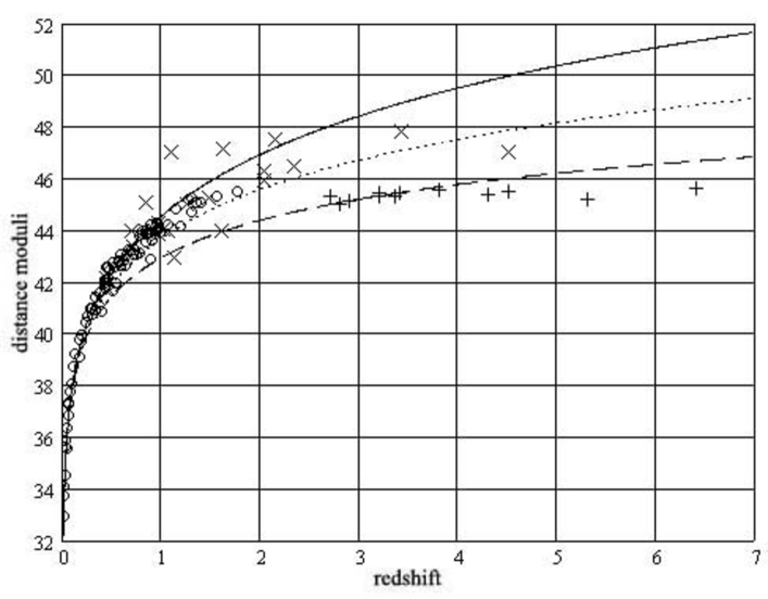
stripe between lower and upper curves. For Fig. 1, supernova observational data (circles, 82 points) are taken from Table 5 of [5], gamma-ray burst observations are taken from [6] (x, 24 points) and from [7] (+, 12 points for $z>2.6$). As it was recently shown by Cuesta et al. [3], the Hubble diagram with $b=1$ (in the language of this paper) gives the best fit to the full sets of gamma-ray burst observations of [6, 7] and it takes place in the standard FLRW cosmology plus the strong energy condition. Twelve observational points of [7] belong to the range $z>2.6$, and one can see (Fig. 1) that these points peak up the curve with $b=0$ which corresponds in this model to the case of very hard radiation in the non-expanding Universe with a flat space. In a frame of models without expansion, any red-shifted source may not be brighter than it is described with this curve.

Figure 2: The difference $\mu_{c}(z)-\mu_{0}(z)$ for $b=1$ (solid) and $b=1.1$ (dot).

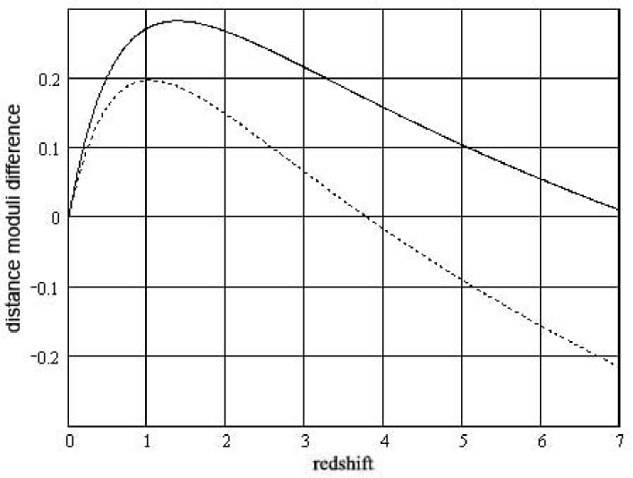
Very recently, Schaefer [8] has published a collection of 69 gamma-ray burst observations where calculated distance moduli are model-dependent: some cosmological model is used to calculate the luminosity distance which is used to evaluate parameters of bursts. When one compares - after it - GRB observations with the used cosmological model constructing the Hubble diagram, one is restricted to be able to check only the self-consistency of the initial conjecture that the chosen model is true. As it is shown in Fig. 2, theoretical distance moduli $\mu_{c}(z)$ for a flat Universe with the concordance cosmology

Figure 3: The same as in Fig. 1 Hubble diagrams $\mu_{0}(z)$ with $b=2.137$ (solid) and $b=0$ (dash); the Hubble diagrams $\mu_{0}(z)$ with $b=1.1$ of this model (dot) and the one of the concordance model (dadot) which is the best fit to observations [8]; GRB observational data (+, 69 points) are taken from Table 6 ($\mu^{a}$) of [8] by Schaefer.

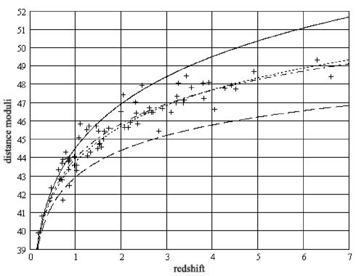
with $\Omega_{M}=0.27$ and $w=-1$, which give the best fit to observations [8], are very close to the Hubble diagram $\mu_{0}(z)$ with $b=1.1$ of this model (the difference is not bigger than $\pm 0.2$ mag in the range $z\leq 6.6$). Because of this, I would like to compare his calculated GRB distance moduli for a flat Universe with the concordance cosmology (see Table 6 of [8]) with theoretical predictions of the considered model in Fig. 3. We can see that GRB observations lie in the stripe between lower and upper curves of this model, and the curve $\mu_{0}(z)$ with $b=1.1$ (or with some bigger $b$) may replace $\mu_{c}(z)$ with a success. But this curve is not the limit case for a very hard radiation. Comparing GRB observational points on Fig. 1 and Fig. 3 for the same range of $z>2.6$, we see also that distance moduli of the last set are essentially higher than the ones reported in [7] by the same author.

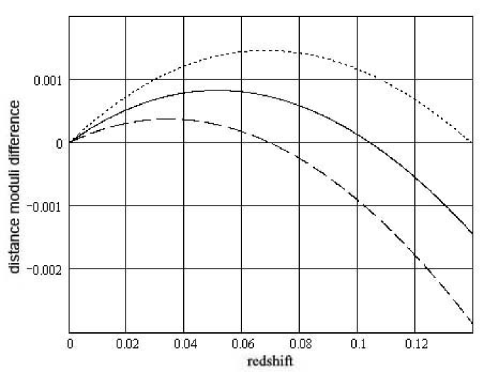
Improved distances to nearby type Ia supernovae (for the range $z<0.14$) can be fitted with the function $\mu_{c}(z)$ for a flat Universe with the concordance cosmology with $\Omega_{M}=0.30$ and $w=-1$ [9]. In Fig. 4, the difference $\mu_{c}(z)-\mu_{0}(z)$ between this function and distance moduli in the considered model is shown for $b=1.52$ (solid), $b=1.51$ (dot) and $b=1.53$ (dash). For $b=1.52$, this difference has the order of $\pm 0.001$ in the considered range of redshifts.

Figure 4: The difference $\mu_{c}(z)-\mu_{0}(z)$ for $b=1.52$ (solid), $b=1.51$ (dot) and $b=1.53$ (dash); $\mu_{c}(z)$ corresponds to a flat Universe with the concordance cosmology with $\Omega_{M}=0.30$ and $w=-1$, which gives the best fit to supernova observations for small redshifts [9].

Results from the ESSENCE Supernova Survey together with other known supernovae 1a observations in the bigger redshift range $z<1$ can be best fitted in a frame of the concordance cosmology in which $\Omega_{M}\simeq 0.27$ and $w=-1$ [10]; the function $\mu_{c}(z)$ for this case is almost indistinguishable from distance moduli in the considered model for $b=1.405$. In Fig. 5, the difference $\mu_{c}(z)-\mu_{0}(z)$ is shown for $b=1.405$ (solid), $b=1.400$ (dot) and $b=1.410$ (dash). For $b=1.405$, this difference is not bigger than $\pm 0.035$ for redshifts $z<1$ (the same is true for slightly different values of $\Omega_{M}$ used in [10], too, but for some other values of the factor $b$: for $\Omega_{M}=0.274$ or 0.267, $b$ is equal to 1.400 or 1.410 correspondingly).

Figure 5: The difference $\mu_{c}(z)-\mu_{0}(z)$ for $b=1.405$ (solid), $b=1.400$ (dot) and $b=1.410$ (dash); $\mu_{c}(z)$ corresponds to a flat Universe with the concordance cosmology with $\Omega_{M}=0.27$ and $w=-1$, which gives the best fit to supernova observations for the bigger redshift range $z<1$ [10].

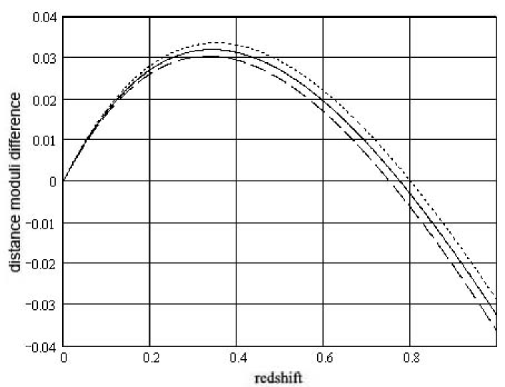
The gold sample of supernovae [5] by Riess et al. has the best fit with $w(z)=w_{0}+w^{{}^{\prime}}z,$ where $w_{0}=-1.31$ and $w^{{}^{\prime}}=1.48$ (dark energy changes with redshift); because this supernovae Hubble diagram goes below of the GRB one [8] for $z>1$, and in a frame of the considered model it is impossible, it may be that the GRB derived distance moduli by Schaefer [8] are not consistent now with the supernovae observations.

3 Conclusion

The considered multivalued character of the Hubble diagram may explain an apparent contradiction between supernovae and GRBs observations. We have now a very poor set of GRBs with big redshifts, and it is obvious that errors of observations are very large. When such missions as the SWIFT satellite observe much more GRBs at high redshifts, one can get a surprising result: observations would lie on the curve which corresponds to the non-expanding Universe. It would be very important to get supernova data for higher redhifts with the help of new missions to be able to do more definitive conclusions.

References

- [1] Riess, A.G. et al. AJ, 1998, 116, 1009.
- [2] Perlmutter, S. et al. ApJ, 1999, 517, 565.
- [3] Cuesta, H.J.M. et al. [astro-ph/0609262].
- [4] Ivanov, M.A. In the book Focus on Quantum Gravity Research, Ed. David C. Moore, Nova Science, New York, 2006, pp. 89-120; [hep-th/0506189 v3]; [http://ivanovma.narod.ru/nova04.pdf].
- [5] Riess, A.G. et al. ApJ, 2004, 607, 665; [astro-ph/0402512].
- [6] Bloom, J.S., Frail, D.A., and Kulkarni, S.R. ApJ, 2003, 594, 674.
- [7] Schaefer, B.E. BAAS, 2005, 37, 1418; 207 AAS Meeting, 2006.
- [8] Schaefer, B.E. [astro-ph/0612285].
- [9] Jha, Saurabh, Riess, A.G. and Kirshner, R.P. [astro-ph/0612666].
- [10] Wood-Vasey, W. M. et al. [astro-ph/0701041].