CHARA Array $K^{\prime}$-band Measurements of the
Angular Dimensions of Be Star Disks

Abstract

We present the first $K^{\prime}$-band, long-baseline interferometric observations of the northern Be stars $\gamma$ Cas, $\phi$ Per, $\zeta$ Tau, and $\kappa$ Dra. The measurements were made with multiple telescope pairs of the CHARA Array interferometer, and in every case the observations indicate that the circumstellar disks of the targets are resolved. We fit the interferometric visibilities with predictions from a simple disk model that assumes an isothermal gas in Keplerian rotation. We derive fits of the four model parameters (disk base density, radial density exponent, disk normal inclination, and position angle) for each of the targets. The resulting densities are in broad agreement with prior studies of the IR excess flux and the resulting orientations generally agree with those from interferometric H$\alpha$ and continuum polarimetric observations. We find that the angular size of the $K^{\prime}$ disk emission is smaller than that determined for the H$\alpha$ emission, and we argue that the difference is the result of a larger H$\alpha$ opacity and the relatively larger neutral hydrogen fraction with increasing disk radius. All the targets are known binaries with faint companions, and we find that companions appear to influence the interferometric visibilities in the cases of $\phi$ Per and $\kappa$ Dra. We also present contemporaneous observations of the H$\alpha$, H$\gamma$, and Br$\gamma$ emission lines. Synthetic model profiles of these lines that are based on the same disk inclination and radial density exponent as derived from the CHARA Array observations match the observed emission line strength if the disk base density is reduced by $\approx 1.7$ dex.

1 Introduction

Be stars are rapidly rotating B-type stars that manage to eject gas into a circumstellar disk (observed in H emission lines, an IR excess flux, and linear polarization; Porter & Rivinius 2003). Be star disks are ephemeral and vary on timescales from days to decades (in some cases disappearing altogether for extended periods). This inherent time variability suggests that gas injection into the disk is only partially the result of the fast spin and equatorial extension of the Be star (Townsend, Owocki, & Howarth, 2004) and that magnetic, pulsational, wind driving, and/or other processes are required for mass loss into the disk (Owocki, 2005). The evolutionary status of Be stars is still a subject of considerable debate (McSwain & Gies, 2005; Zorec, Frémat, & Cidale, 2005), but there is growing evidence that many Be stars were spun up through mass transfer from a binary companion that has since become a neutron star, white dwarf, or hot subdwarf (Pols et al., 1991; Gies, 2000).

The direct resolution of Be star disks has come through high resolution radio observations ($\psi$ Per; Dougherty & Taylor 1992) and long baseline interferometry in a narrow band around the H$\alpha$ emission feature (Stee et al., 2005). The first H$\alpha$ studies focused on the bright, northern sky Be stars $\gamma$ Cas (Thom, Granes, & Vakili, 1986; Mourard et al., 1989; Stee et al., 1995; Berio et al., 1999) and $\zeta$ Tau (Vakili et al., 1998). In a seminal paper, Quirrenbach et al. (1997) presented results for seven Be stars based upon narrow-band H$\alpha$ observations made with the MkIII interferometer at Mount Wilson Observatory. They were able to resolve the disks around all seven stars, and they found diameters in the range $2.6-4.5$ mas (Gaussian FWHM). In most cases the visibilities indicated an elongated shape; for example, in the case of $\zeta$ Tau, the major axis was resolved (4.53 mas diameter) but the orthogonal minor axis remained unresolved, consistent with the suggestion that we are viewing the disk almost edge-on.  The disk orientation position angle on the sky inferred from polarimetry matched the interferometric results in every case.  These results have been extended and improved through new interferometric observations with the Navy Prototype Optical Interferometer (NPOI) in an important series of papers by Tycner and collaborators (Tycner et al., 2003, 2004, 2005, 2006).

The relative flux contribution from the disk becomes larger in the infrared spectral range due to bound-free and free-free emission from the dense and ionized gas in the disk. Waters (1986) developed a disk model for the IR emission that he subsequently applied to determine the disk properties of 101 Be stars based upon their far-IR emission observed with the IRAS satellite (Coté & Waters, 1987; Waters, Coté, & Lamers, 1987), and Dougherty et al. (1994) further extended this analysis to study the near-IR excess in 144 Be stars. Howells et al. (2001) demonstrated that the near-IR flux excess is correlated with the H$\alpha$ emission strength in Be stars as expected for a common origin in the disk. Thus, the near- and mid-IR ranges (Rinehart, Houck, & Smith, 1999) offer a new opportunity for resolving the disks of Be stars through long baseline interferometry. Stee & Bittar (2001) presented a wind model for the infrared emission from Be stars and the corresponding interferometric visibilities for the models.  Their model for $\gamma$ Cas, for example, predicts that the disk should appear approximately two times larger in the $K$-band continuum and in the Br$\gamma$ emission line than found by narrow-band H$\alpha$ interferometry. Stee (2003) made additional predictions for 16 Be stars of the expected $K$-band interferometric visibilities. The first attempt to resolve the infrared disk flux was recently made by Chesneau et al. (2005) who made $N$-band observations with the VLTI/MIDI instrument of the bright southern Be star $\alpha$ Ara, and their results indicate that the disk is smaller than that predicted by Stee (2003), perhaps due to disk truncation by a faint binary companion. $K$-band interferometric observations from VLTI/VINCI of $\alpha$ Ara were reported by Domiciano de Souza et al. (2003) who interpreted the visibilities using a rotationally distorted photospheric model.

Here we present the first near-IR interferometric observations of four bright, northern sky Be stars that we obtained with the Georgia State University Center for High Angular Resolution Astronomy (CHARA) Array at Mount Wilson Observatory (McAlister et al., 2005; ten Brummelaar et al., 2005). We describe the interferometric and complementary spectroscopic observations in §2 and then we present a simple disk model in §3 that we use to predict the interferometric visibilities and spectral line profiles. We discuss the specific results for each of the four targets in §4. Our results are summarized in §5.

2 Observations

2.1 Targets

We selected four well known Be stars for this initial program of CHARA Array interferometry: $\gamma$ Cas (HR 264 = HD  5394 = HIP 4427), $\phi$ Per (HR 496 = HD 10516 = HIP 8068), $\zeta$ Tau (HR 1910 = HD 37202 = HIP 26451), and $\kappa$ Dra (HR 4787= HD 109387 = HIP 61281). All the targets except $\kappa$ Dra have prior narrow-band H$\alpha$ interferometric observations (Quirrenbach et al., 1997; Tycner et al., 2003, 2004, 2006). The first three stars were targets in speckle interferometric searches for close companions, and no such companions were detected (Mason et al., 1997); however, oscillations in the the proper motion of $\gamma$ Cas suggest the presence of a faint companion with a period of some 60 y (Gontcharov, Andronova, & Titov, 2000). On the other hand, all four of the targets are known spectroscopic binaries with periods in the range 61 – 204 d. The companion in the case of $\phi$ Per is a hot subdwarf whose spectral features appear in the UV spectrum (Gies et al., 1998), but for the other three stars the nature of the low mass companion is unknown.

We summarize the adopted parameters for the target stars in Table 1 that lists the spectral classification, parallax (Perryman, 1997), radius, mass, effective temperature, and projected rotational velocity (Yang et al., 1990; Abt, Levato, & Grosso, 2002) of the bright primary star. The next three rows give the radius, mass, and effective temperature of the secondary. These are only known for $\phi$ Per and representative values are listed for the others assuming that they also have hot subdwarf companions (see §3.3). The next four rows list the binary period, epoch of the secondary star’s maximum radial velocity (equal to the epoch of the secondary’s crossing of the ascending node), the primary star to center of mass portion of the semimajor axis, and the adopted Roche radius of the primary star. The final row provides a key to the references from which these various parameters were adopted.

2.2 $K^{\prime}$-band Interferometry from the CHARA Array

The CHARA Array observations were made on various dates during the first two years of operation (Table 2). The telescope, instrumentation, and data reduction procedures are described in detail by ten Brummelaar et al. (2005). The CHARA Array consists of six 1 m telescopes in a $Y$-configuration with pairwise baselines ranging from 34 to 330 m in length. The Be star observations were primarily made with intermediate to long baseline configurations using the $K^{\prime}$ filter described by McAlister et al. (2005). A summary of each night’s observations is given in Table 2 that lists the target and calibrator star names, the telescope pair (with the maximum baseline given in meters in parentheses; ten Brummelaar et al. 2005), the UT date, and the number of sets of measurements. We made the measurements using the “CHARA Classic” beam combiner, which is a two-beam, pupil-plane (or Michelson) combiner (Sturmann et al., 2003). The fringes were recorded with a near-IR detector on either 1 or $2\times 2$ pixels at a sampling rate of 100 or 150 Hz depending on the seeing conditions. The path length scans were adjusted to obtain approximately five samples per fringe spacing. Each measurement set consists of some 200 scans of the fringe pattern with photometric calibration scans performed before and after. The raw visibilities were estimated from an edited set of scans using the log-normal power spectrum method described by ten Brummelaar et al. (2005).

We transformed the raw visibilities into absolute visibility $V$ by interleaving the target observations with measurements of calibrator stars with small angular diameters (Berger et al., 2006). The calibrator stars are generally close in the sky and of comparable $K^{\prime}$ magnitude to the targets, and we list in Table 3 their effective temperatures and gravities as derived by other investigators (identified in column 7). We estimated the angular diameters of the calibrator stars by comparing their observed and model flux distributions. The angular diameter of the limb darkened disk $\theta_{LD}$ (in units of radians) is found by the inverse-square law:

$${{f_{\lambda}({\rm observed})}\over{F_{\lambda}({\rm emitted})~{}10^{-0.4A_{\lambda}}}}=({R_{\star}/d})^{2}={1\over 4}\theta_{LD}^{2}$$ (1)

where the ratio of the observed and emitted fluxes (reduced by the effects of interstellar extinction $A_{\lambda}$) depends on the square of the ratio of stellar radius $R_{\star}$ to distance $d$. Most of the calibrator stars are relatively close by and the interstellar extinction is negligible. The one exception is HD 107193, and in this case we adopted an extinction curve law from Fitzpatrick (1999) that is a function of the reddening $E(B-V)$ and the ratio of total-to-selective extinction $R=A_{V}/E(B-V)$ (set at a value of 3.1).

The model fluxes were interpolated from the grid of models from R. L. Kurucz based upon the values of $T_{\rm eff}$ and $\log g$ in Table 3. These model fluxes are based upon solar abundance, plane-parallel, local thermodynamic equilibrium (LTE), line blanketed atmospheres with a microturbulent velocity of 4 km s^-1 that should be adequate for these A- and F-type main sequence stars. We compiled data on the observed fluxes from the optical to the near-IR. We found Johnson $UBV$ photometry for all the calibrators, and these magnitudes were transformed to fluxes using the calibration of Colina, Bohlin, & Castelli (1996). We also included Strömgren photometry for several calibrators using the calibration of Gray (1998). Spectrophotometry from Kharitonov, Tereshchenko, & Knyazeva (1988) was used for HD 6210. All of the stars are included in the 2MASS All-Sky Catalog of Point Sources (Cutri et al., 2003), and we converted the $JHK$ magnitudes to fluxes using the calibration of Cohen, Wheaton, & Megeath (2003). In a few cases the errors in the 2MASS magnitudes were unacceptably large, and we relied instead on IR fluxes from the COBE DIRBE instrument (Smith, Price, & Baker, 2004). The angular diameters we derived by fitting the spectral energy distributions are given in column 6 of Table 3. Most of these calibrators have angular diameters that are small enough that their associated errors will introduce only minor systematic errors in our derived target angular sizes (van Belle & van Belle, 2005).

It is normal practice in interferometry to estimate the actual visibility of a calibrator by adopting a uniform disk function for the visibility curve as a function of wavelength and baseline, but in fact it is no more difficult to apply a visibility curve for a limb darkened disk provided the form of the limb darkening is known (Davis, Tango, & Booth, 2000). We used the effective temperatures and gravities from Table 3 to estimate the $K$-band limb darkening coefficients from the tables of Claret (2000), and then we calculated the limb darkened visibility curves for the calibrators (for the projected baseline at the time of observation and the limb darkened angular diameter given in Table 3) by making a weighted sum of the predicted visibilities over the wavelength band of the $K^{\prime}$ filter (to account for bandwidth smearing). We then made a simple linear interpolation in time between the target and calibrator observations to estimate the ratio of raw to absolute visibility required to transform the results to absolute visibility. Note that we also made a spline fit of the time evolution of calibrator visibility, and the difference between the spline and linear interpolated visibilities was added quadratically to the error budget for the final calibrated visibility to help estimate the errors introduced by the time interpolation scheme.

The calibrated visibilities are presented in Table 4 (available in full in the electronic version of the paper). The columns in this table give the target name, the heliocentric Julian date of the mid-point of the data set, the binary orbital phase determined from the period and epoch given in Table 1, the telescope pair used for the observation, the projected baseline and position angle of the target as viewed from the telescope pair at the mid-point time, and the calibrated visibility. Note that the visibility errors quoted represent the internal errors from the power spectrum analysis of the fringes plus a term introduced for the calibration process, and these may underestimate the actual visibility errors. We find, for example, that there are some closely spaced observations on certain nights with comparable projected baselines and position angles that have a scatter that is several times larger than the formal errors. There are 11 such subsets of 4 or more measurements from within a specific night that have ranges of $\delta({\rm baseline})<10$ m and $\delta({\rm position~{}angle})<10^{\circ}$, and the average ratio of the standard deviation of $V$ within a subset to the mean of the quoted internal error in $V$ is a factor of 2.8. Thus, the quoted errors are probably lower limit estimates of the true error budget.

2.3 Optical Spectroscopy

The disks of Be stars exhibit large temporal variations in their H-Balmer emission strengths that presumably reflect large structural changes in their geometry and/or density (Porter & Rivinius, 2003). Thus, we obtained new spectroscopic observations of the target Be stars in order to compare the Balmer emission levels at times contemporaneous with the interferometric observations. The sources and details of the spectroscopy are listed in Table 5 that reports the observatory and telescope of origin, the spectroscopic instrument, spectral resolving power $R=\lambda/\delta\lambda$, spectral range recorded, UT dates, and the names of targets. Most of the observations of the H$\alpha$ and H$\gamma$ lines were made with the Kitt Peak National Observatory (KPNO) coudé feed telescope, and these have moderate resolution and high S/N properties. The H$\alpha$ spectra of $\kappa$ Dra were obtained at both the University of Toledo Ritter Observatory and the Ondřejov Observatory at the same time as the first CHARA Array observations were made, and a low dispersion blue spectrum was also obtained at that time with the University of Texas McDonald Observatory 2.7 m telescope (recording H$\beta$ through the higher Balmer sequence). All of these spectra were reduced using standard routines in IRAF to create continuum rectified versions of each spectrum. The atmospheric telluric lines in the vicinity of H$\alpha$ were removed from the KPNO coudé feed spectra (Gies et al., 2002), but these features were quite weak in the $\kappa$ Dra H$\alpha$ spectra and were left in place. We describe these Balmer line profiles in §4 and §5 below.

2.4 $K$-band Spectroscopy

The IR excess flux from Be star disks will tend to dilute the photospheric and emission lines in the near-IR spectral range, and the strength of the Br$\gamma$ emission line in particular offers a sensitive test of the IR excess fluxes derived from interferometry. Thus, we also obtained low resolution $K$-band spectroscopy of all the targets except $\kappa$ Dra with the University of Texas McDonald Observatory 2.7 m telescope and CoolSpec spectrometer (Lester et al., 2000). We used a $1\farcs 0$ entrance slit and a grating with 75 grooves mm^-1 in second order, yielding a spectral resolving power of $R\approx 1520$ (Table 5). The detector was a NICMOS3 HgCdTe $256\times 256$ pixel array. The spectra were reduced using the methods described by Likkel et al. (2006) except that in our case the sky background was estimated from the intensity at off-star positions along the projected slit.

We also made a number of spectra at different air masses of the broad-lined, A0 V stars HR 567 (HD 11946) and HR 2398 (HD 46553), which we used to remove the numerous atmospheric features in this spectral band. The stellar spectra of these two stars are essentially featureless with the exception of the photospheric Br$\gamma$ line (Wallace & Hinkle, 1997), and we formed pure atmospheric spectra by dividing our observed spectra by the average stellar spectra of the similar stars HR 5793 and HR 7001 (after broadening for the lower resolution of our spectra and for the higher projected rotational velocities of HR 567 and HR 2398) that we obtained from the spectral library of Wallace & Hinkle (1997). The target spectra were then divided by these atmospheric spectra (after small line depth corrections to account for differing air masses) to obtain the final continuum rectified versions that are presented below (§5).

3 Be Star Disk Models

The observed interferometric visibilities can be interpreted by assuming that the Be star disks have a relatively simple spatial intensity in the sky, perhaps a uniform ellipsoid, ring, or Gaussian ellipsoid (Tycner et al., 2006). However, the quality of the interferometric data is sufficient to begin to explore more physically motivated models for the disk appearance. Here we present a relatively simple model for the near-IR emission that is derived from the Be circumstellar disk model of Hummel & Vrancken (2000). The advantages of this approach are that we can compare the resulting disk gas densities with prior work on the near-IR spectrum and that we can also predict the disk emission line strengths for comparison with our observed spectra. In the following subsections we outline the basic assumptions and characteristics of the model that we then apply to fit the CHARA Array observations of visibility. We discuss the model predictions for spectroscopy below in §4.

3.1 Disk Geometry and Model Parameters

Hummel & Vrancken (2000) present a simple model for the circumstellar disks of Be stars that they use to explore the emission line shapes. The basic concept is that the disk is axisymmetric and begins at the stellar surface. The gas density in the disk is given by

$$\rho(R,Z)=\rho_{0}R^{-n}\exp\left[-{1\over 2}\left({Z\over{H(R)}}\right)^{2}\right]$$ (2)

where $R$ and $Z$ are the radial and vertical cylindrical coordinates (in units of stellar radii), $\rho_{0}$ is the base density at the stellar equator, $n$ is a radial density exponent, and $H(R)$ is the disk vertical scale height. This gas scale height is given by

$$H(R)={C_{S}\over V_{K}}R^{3\over 2}$$ (3)

where $C_{S}$ is the sound speed and $V_{K}$ is the Keplerian velocity at the stellar equator. We assume that the outer boundary of the disk occurs at a radius $R_{d}$ that is equal to the Roche radius of the Be star for these four binary targets (Table 1). This assumption is probably more critical for the mid-IR emission spectrum, but it not important for the $K^{\prime}$ emission that is generally confined to regions well within the Roche radii of our targets.

Hummel & Vrancken (2000) assume that the temperature is constant throughout the disk and is given by $T_{d}={2\over 3}T_{\rm eff}$ where $T_{\rm eff}$ is the stellar effective temperature. In fact, recent physical models for Be disks by Carciofi & Bjorkman (2006) show that the gas temperature is actually a function of both $R$ and $Z$, but their work shows that the temperature is about $60\%~{}T_{\rm eff}$ in the outer, optically thin parts of the disk, so we adopt this value for the isothermal approximation used here.

We assume that the star itself is spherical and of uniform brightness in the $K^{\prime}$ band. Neither of these assumptions is probably correct for a rotationally distorted and gravity darkened Be star (Townsend et al., 2004), but the photospheres of the targets are small enough (see Table 6 below) that these details are inconsequential for the baselines and wavelength of the CHARA Array observations. We suppose that the disk is observed with the disk normal oriented to our line of sight with an inclination angle $i$ and a position angle $\alpha$ measured east from north in the sky. Note that this position angle convention is $90^{\circ}$ different from that adopted in the H$\alpha$ interferometric studies where the position angle of the projected major axis is usually given. Thus, the four parameters that define a disk model are the base density $\rho_{0}$, the density exponent $n$, and the orientation angles $i$ and $\alpha$.

3.2 $K^{\prime}$-band Continuum Images and Interferometric Visibility

We determine the surface brightness of the disk plus star over a projected rectilinear coordinate grid on the sky by solving the equation of transfer along a ray through the center of each grid position,

$$I=S_{d}(1-e^{-\tau})+I_{\star}e^{-\tau}$$ (4)

where $I$ is the derived specific intensity, $S_{d}$ is the source function for the disk gas (taken as the Planck function for the disk temperature $T_{d}$), $I_{\star}$ is the specific intensity for a uniform disk star (taken as the Planck function for $T_{\rm eff}$), and $\tau$ is the integrated optical depth along the ray. The main shortcoming in this expression is the neglect of a scattered light term to account for Thomson scattering of photospheric intensity (see, for example, eq. [6] in Bjorkman & Bjorkman 1994). For the typical electron densities that we find for our Be star targets, this term will amount to only a few percent of the stellar specific intensity at locations close to the star, which is usually much less than the disk source function in the optical thick portions, so this simplification is acceptable in the $K^{\prime}$ band.

The disk optical depth in the near-IR is predominantly due to bound-free and free-free processes, and we can express the increment in optical depth with an incremental step $ds$ along a given ray as

$$d\tau=C(\lambda,T_{d})\rho(R,Z)^{2}~{}ds$$ (5)

where the coefficient $C(\lambda,T_{d})$ is given by equation (5) in Dougherty et al. (1994) (see also Waters 1986). This coefficient includes terms for the Gaunt factors for bound-free and free-free emission that we evaluated for the $K^{\prime}$ band using the tables in Waters & Lamers (1984). We adopted an ionization model for the disks of the two hotter Be stars, $\gamma$ Cas and $\phi$ Per, that assumed ionized H, singly-ionized He, and doubly-ionized C, N, and O atoms, while for the cooler Be stars, $\zeta$ Tau and $\kappa$ Dra, we assumed ionized H, neutral He, and singly ionized C, N, and O. Note that we evaluated the optical depth coefficient only at the central wavelength of the $K^{\prime}$ filter since the coefficient varies slowly with wavelength. Also note that we have accounted only for continuum emission in this band since the Br$\gamma$ emission contribution is small compared to the flux integrated over the $K^{\prime}$ band (§5).

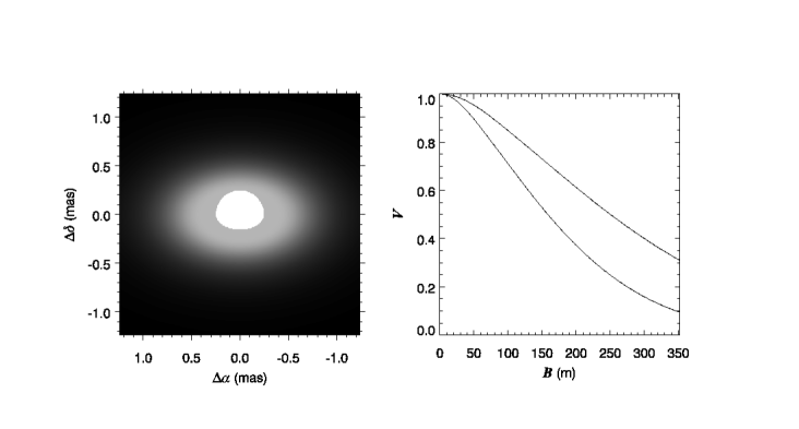
Figure 1: The left panel is a depiction of the $K^{\prime}$ image of a disk model for the case of $\gamma$ Cas ($i=51^{\circ}$, $\rho_{0}=7.2\times 10^{-11}$ g cm^-3, $n=2.7$). The right panel shows the corresponding interferometric visibility $V$ as a function of projected baseline for position angles along the apparent minor axis (top line) and major axis (bottom line).

The image of the Be star in the sky in constructed by integrating the optical depth along each ray according to equations (2) and (5), and then populating each pixel of the image using equation (4). The pixel scale on the sky is set by the adopted angular diameter of the star (derived from the parallax and radius in Table 1). We show an example calculation for $\gamma$ Cas in the left panel of Figure 1. Portions of the disk projected against the sky include only the first term of equation (4), and the disk intensity attains a maximum of $S_{d}\approx 55\%I_{\star}$ in the inner optically thick regions. At a radius where the optical depth is approximately unity, the disk becomes optically thin and fades with increasing radius. Part of the background disk is occulted by the star while the part in foreground attenuates the photospheric intensity. We also include a binary star option to add the disk of a secondary into the image at a position appropriate for the time of observation.

The interferometric visibilities are then calculated by making Fourier transforms of such disk images, and we did this following the techniques described by Aufdenberg et al. (2006). The comparison with the observed visibility is done by determining the discrete Fourier transform of the image for the $(u,v)$ spatial frequency pair of the observation (see eq. [19] in Aufdenberg et al. 2006), and this calculation is done successively and summed over five wavelength bins according to the transmission curve of the $K^{\prime}$ filter (McAlister et al., 2005). This procedure assumes that spectral energy distributions in the $K^{\prime}$ band of our targets are similar to the stellar transmission curve (Rayleigh-Jeans tail), and this is probably acceptable in the $K^{\prime}$ band where the disk emission is just beginning to become an important component of the total flux (Waters, 1986). The Fourier transforms along the major and minor axes of the projected disk image for the $\gamma$ Cas example are illustrated in the right hand panel of Figure 1 (here without accounting for bandwidth smearing). The top curve shows the slower decline in $V$ for the smaller minor axis while the bottom curve illustrates the rapid decline for the better resolved major axis. Note that the star itself is so small ($\theta_{LD}=0.50$ mas) that its visibility curve in the absence of a disk would decline to only $V=0.87$ at a baseline of 300 m.

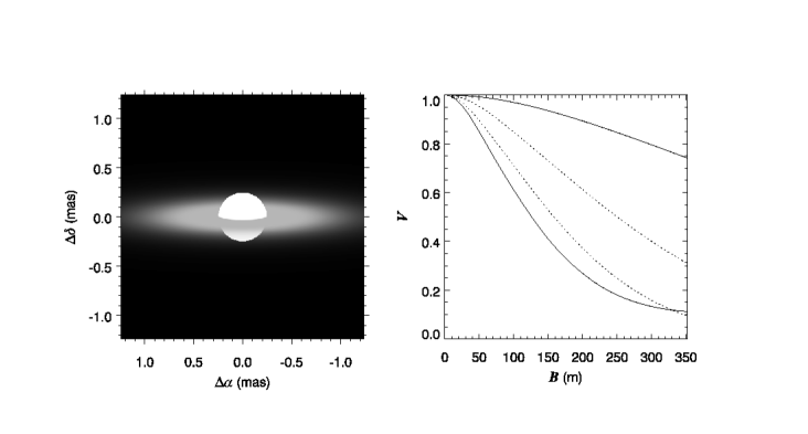
Figure 2: An image and visibility plots for a $\gamma$ Cas model as in Fig. 1 but with a larger inclination of $i=80^{\circ}$. The dotted lines in the visibility panel repeat the curves from the original model in Fig. 1.

Figure 2 shows how the image and visibilities change by altering the disk inclination angle from $51^{\circ}$ to $80^{\circ}$ (the dotted lines in the right hand panel copy the original visibility curves from Fig. 1). The rays through the outer positions along the major axis now traverse more optical depth because of the oblique view through the disk, and this brightens the outer regions making the disk effectively larger in this dimension (so that the decline in $V$ with baseline is steeper). On the other hand, the minor axis now appears more foreshortened and the visibility decline is reduced. Thus, the $V$ variation with position angle in the sky (with respect to the major axis) is very sensitive to the disk inclination angle $i$.

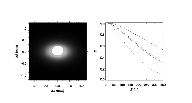
Figure 3: An image and visibility plots for a $\gamma$ Cas model as in Fig. 1 but with a smaller base density of $\rho_{0}=3.6\times 10^{-11}$ g cm^-3. The dotted lines in the visibility panel repeat the curves from the original model in Fig. 1.

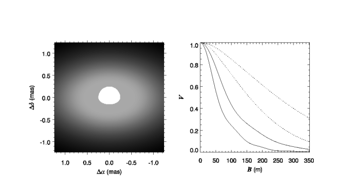
Figure 4: An image and visibility plots for a $\gamma$ Cas model as in Fig. 1 but with a smaller radial density exponent of $n=2.0$. The dotted lines in the visibility panel repeat the curves from the original model in Fig. 1.

The changes resulting from a decrease in disk base density $\rho_{0}$ are illustrated in Figure 3. Now the density is lower throughout the disk, and consequently the optically thick part of the disk appears smaller in both dimensions (and the $V$ curves decline more slowly with baseline). Changes in the opposite sense result from a decrease in the density exponent as shown in Figure 4 (from $n=2.7$ to 2.0). The radial density decline is less steep in this case so that much more of the inner disk is optically thick, leading to a larger appearance in the sky (steeper decline in the $V$ curves). These examples show that the visibility curves are most sensitive to the disk size as given by the boundary between the optically thick and thin regions. Since the optical depth unity radius in the disk plane depends on $\rho_{0}^{2}r^{-2n+3/2}$, there will be a locus of parameters that will produce visibility curves with similar decline rates in the main lobe and with subtle differences appearing only at intermediate and longer baselines. Thus, accurate determinations of both $\rho_{0}$ and $n$ will require visibility measurements over a broad range of baselines.

3.3 Model Fitting Results

We found best fit solutions for the four disk parameters by fitting the model and observed $K^{\prime}$ visibilities using a numerical grid search technique. We used an iterative search on each of the individual parameters to find the set that provided the lowest overall $\chi^{2}_{\nu}$ statistic. The results are listed in Table 6 for both single star and binary star models (see below). The seventh row of Table 6 reports the minimum $\chi^{2}_{\nu}$ values, and these are all much larger than the expected value of unity for acceptable fits. Recall that the internal errors on $V$ may underestimate the actual errors by a factor of 2.8 for these measurements (§2.2), so we might instead expect to find best fits with $\chi^{2}_{\nu}\approx 2.8^{2}=7.84$. This is more or less consistent with the fitting results for all but $\gamma$ Cas, where the residuals are still larger than expected. We estimated the errors in the fitting parameters by renormalizing the minimum $\chi^{2}_{\nu}$ to unity and then finding the excursion in the parameter that increased $\chi^{2}_{\nu}$ to a value of $1+1/(N_{V}-4)$ (for $N_{V}$ visibility measurements and 4 fitting parameters). Since the disk parameters $\rho_{0}$ and $n$ are so closely coupled in the fits (§3.2), we searched the locus of the pair-wise fits for the same increase in $\chi^{2}_{\nu}$, and we quote the half-range in these parameters for their errors.

The first two rows of Table 6 give the orientation parameters, the disk plane normal inclination $i$ and position angle $\alpha$ (east from north). Note that there is a $180^{\circ}$ ambiguity in the value of $\alpha$ (i.e., whether the disk north pole is in the eastern or western half of the sky), so we assume the range $0\leq\alpha<180^{\circ}$. The third and fifth rows list the logarithm (base 10) of the disk base density $\log\rho_{0}$ and the disk density exponent $n$, respectively (base electron density is $\log N_{e}=\log\rho_{0}+23.6$). These are compared with the same parameters in rows four and six, respectively, estimated from model fits of the IR flux excess from IRAS observations that were computed by Waters et al. (1987). Waters et al. (1987) make a number of simplifying assumptions about the disk geometry that make a direct comparison of results unreliable, but in general there is reasonable agreement except in the two cases where a binary companion may influence the results, $\phi$ Per and $\kappa$ Dra (see below). Row 8 gives a derived model quantity related to the IR flux excess, $E(V-K)=2.5\log(1+F_{d}/F_{\star})$, where $F_{d}$ and $F_{\star}$ are the integrated disk and stellar flux, respectively. If we assume that the disk flux is relatively small in the optical, then this quantity can be directly compared to the observed IR flux excess measurements by Dougherty et al. (1994) that are listed in row 9. The model and observed values of $E(V-K)$ are comparable but not always a good match. We suspect the differences may relate to the temporal variations in the disk emission (from $\sim 1990$ for the IR magnitudes to $\sim 2005$ for the CHARA Array measurements). Rows 10 and 11 compare the adopted stellar angular diameter $\theta_{LD}$ with the model disk emission FWHM diameter along the projected major axis. The disk emission FWHM was estimated from the width at $50\%$ of the emission intensity in the optically thick part just above the photosphere.

We know that all four targets are close binaries with faint, low-mass companions, but the nature of the companion is only known in the case of $\phi$ Per (Gies et al., 1998). The secondary of $\phi$ Per is a hot helium star, the stripped down remains of what was once the more massive star before mass transfer began. If we assume that all our Be star targets are likewise the mass gainers that have been spun up by the angular momentum carried with mass transfer, then they may also have helium star companions (or possibly white dwarf or neutron star companions). We present here a sample calculation of how such a binary companion would affect the $K^{\prime}$ visibilities. For the purpose of this demonstration, we assume that the companion is a hot ($T_{\rm eff}=30000$ K) and small ($R=1R_{\odot}$) helium star (except in the case of $\phi$ Per where we have better estimates for these parameters; see Table 1). According to the interacting binary scenario, the angular momentum vector of the mass gainer Be star should be parallel with the orbital angular momentum vector, so the disk plane corresponds to the orbital plane. Consequently, we can apply the orientation parameters for the disk, $i$ and $\alpha$, also to the orbit of the secondary. We know the epoch of the secondary’s ascending node passage from the spectroscopic radial velocity curves (Table 1), so the only remaining unknown for the secondary’s astrometric orbit is the sense of motion on the sky (increasing or decreasing position angle with time). We follow the normal convention of assigning an inclination in the range $0^{\circ}\leq i<90^{\circ}$ for counterclockwise apparent motion and in the range $90^{\circ}<i\leq 180^{\circ}$ for clockwise motion (so that the longitude of the node is $\Omega=\alpha+270^{\circ}$ for $i<90^{\circ}$ and $\Omega=\alpha+90^{\circ}$ for $i>90^{\circ}$). We made fits of the visibility for these two binary orbit cases, and we show in Table 6 the results for the best fit sense of motion. The minimum $\chi^{2}_{\nu}$ was significantly reduced only for the case of $\phi$ Per (where the properties of the secondary are known; the estimated magnitude difference is $\triangle K^{\prime}=2.9$ mag). The inclusion of the binary companion also resulted in a significant change in the fitted disk properties for $\kappa$ Dra (discussed further in §5.4).

It is valuable to compare the $K^{\prime}$ angular diameters with those derived from narrow-band H$\alpha$ interferometry, and to do so we need to fit the visibilities with a simple Gaussian ellipsoidal model as done for the H$\alpha$ results. We made these fits also by a numerical grid search of the four parameters that describe the Gaussian ellipsoidal model: the angular FWHM of the major axis $\theta_{\rm GD}$, the ratio of the minor to major axes $r$ ($\geq\cos i$), the position angle of the major axis $\phi$ ($=\alpha\pm 90^{\circ}$), and the fraction of the total flux contributed by the photosphere of the Be star $c_{\rm P}$. The best fit results are listed in Table 7 for these single star models. Our results are compared with those from Quirrenbach et al. (1997) and Tycner et al. (2004, 2006) based on interferometric observations of the H$\alpha$ emission, and the orientation parameters appear to be in reasonable agreement. We find, however, that the $K^{\prime}$ disk diameters are somewhat smaller than the H$\alpha$ diameters ($\approx 64\%$ as large), contrary to the wind model predictions of Stee & Bittar (2001). Note that the $\chi_{\nu}^{2}$ residuals of the Gaussian elliptical fits are comparable to those from the physical model fits (Table 6), and additional longer baseline observations will be required to distinguish between them.

4 Model Emission Lines and Spectroscopy

We can also use the simple disk model to estimate the line profiles of the disk emission lines (Hummel & Vrancken, 2000). However, the problem is now more complex because of the wavelength dependence of the emission, and a number of key assumptions about the atomic populations must be made. Despite these difficulties, it is nevertheless interesting to check whether or not the disk density parameters derived from interferometry lead to predicted line profiles that are consistent with the observed ones. Here we discuss the line synthesis predictions for the disk models and their comparison with our spectroscopic observations.

4.1 Disk Emission Line Models

The line synthesis procedure has many similarities with the disk image calculations present above. We assume the same basic density law (eq. [2]), the same creation of a rectilinear grid of points covering the projected positions of the star and disk in the sky, and the solution of the equation of transfer (eq. [4]) along along a ray through the center of each grid point. However, for the line synthesis the expression for the optical depth (eq. [5]) becomes (Hummel & Vrancken, 2000)

$$d\tau_{\lambda}={{\pi e^{2}}\over{mc}}f\lambda_{0}~{}N(H_{i})~{}P_{\lambda}(V_{r},N_{e})~{}ds$$ (6)

and now we consider a wavelength dependent optical depth $\tau_{\lambda}$ for the region surrounding an emission line (we adopt an equivalent radial velocity grid in 10 km s^-1 increments from $-2000$ to $+2000$ km s^-1). The first term in the expression is the scattering coefficient for a classical oscillator that is multiplied by the oscillator strength $f$ and the rest wavelength $\lambda_{0}$ for the specific transition (H$\gamma$, H$\alpha$, and Br$\gamma$).

The next term $N(H_{i})$ is the local number density of neutral H atoms in energy level $i$. This can be set approximately by balancing the recombination rate with the photoionization rate (for the case when all the bound-bound transitions are very optically thick; Cassinelli, Nordsieck, & Murison 1987)

$$\alpha(T)N_{e}N_{p}=N_{i}\int\limits_{\nu_{0}}^{\infty}{{4\pi}\over{h\nu}}a_{\nu}J_{\nu}~{}d\nu$$ (7)

where $\alpha(T)$ is the recombination coefficient, $N_{e}$ and $N_{p}$ are the electron and proton number densities, $N_{i}$ is the number density of hydrogen in energy level $i$, $a_{\nu}$ is the photoionization cross section, and $J_{\nu}$ is the mean radiation field. If we assume that the latter results only from unattenuated starlight, then the mean field at a distance $r$ from the star can be written

$$J_{\nu}=W(r)I_{\nu}^{\star}$$ (8)

where $W(r)$ is the dilution factor given by

$$W(r)=0.5(1-[1-r^{-2}]^{1\over 2}),$$ (9)

$r$ is the radial distance from the star $r=(R^{2}+Z^{2})^{1\over 2}$, and $I_{\nu}^{\star}$ is the stellar specific intensity. Cassinelli et al. (1987) rewrite the photoionization/recombination equilibrium to express the level population $N_{i}$ in terms of a variable $q_{i}$,

$$N_{i}=N_{e}N_{p}~{}\alpha(T)/\int\limits_{\nu_{0}}^{\infty}{{4\pi}\over{h\nu}}a_{\nu}W(r)I_{\nu}^{\star}~{}d\nu\equiv N_{e}N_{p}q_{i}.$$ (10)

In the stellar photosphere, $W(r)=1$, $I_{\nu}^{\star}=B_{\nu}(T_{\rm eff})$ (the Planck function), and the gas will be in LTE, so that $q_{i}^{\rm LTE}=N_{i}/(N_{e}N_{p})$ will be given by the Boltzmann-Saha equation. In the circumstellar disk, the photoionization rate will vary with $W(r)$ and the recombination rate will depend on $\alpha(T)\propto T^{-1/2}$, so level populations will be given by

$$N_{i}=q_{i}^{\rm LTE}\sqrt{T_{\rm eff}/T_{d}}~{}N_{e}N_{p}/W(r).$$ (11)

The actual populations probably have a more complex dependence on position in the disk (Carciofi & Bjorkman, 2006).

The final term in optical depth equation is the normalized line profile $P_{\lambda}(V_{r},N_{e})$ that depends on the local radial velocity $V_{r}$, electron density, and the adopted temperature of the isothermal disk $T_{d}$. We adopted the convolved thermal and Stark broadened profiles calculated by T. Schöning and K. Butler for H$\alpha$ and H$\gamma$, but we used only a simple thermal profile for Br$\gamma$. These profiles were collected into a matrix of 401 wavelength points (corresponding to our radial velocity grid), 60 positive Doppler shifts (in increments of 10 km s^-1), and four electron number densities ($\log N_{e}=[10.5,12,13,14]$).

The line synthesis calculation proceeds by solving for the intensity spectrum from each pixel in the projected image and then summing these to create a predicted flux profile. At each position along a ray through a pixel, we determine the Keplerian velocity and Doppler shift, gas density, H population, and profile shape (simply adopting the closest match in the grid), and then we integrate the optical depth for each wavelength point. The summed spectral intensity is then found through equation (4), but in this calculation $I_{\star}$ is replaced with a specific intensity corresponding to a photospheric absorption line with the corresponding value of surface normal orientation and Doppler shift for the projected position. These intensity profiles were calculated by first creating line blanketed LTE model atmospheres using the ATLAS9 program written by Robert Kurucz. These models assume a stellar temperature and gravity derived from the parameters in Table 1, solar abundances, and a microturbulent velocity of 2 km s^-1. Then a series of specific intensity spectra were calculated using the code SYNSPEC (Hubeny & Lanz, 1995) for each of these models and H lines. These profiles include the effects of limb darkening for the stellar photosphere. Because our model assumes axial symmetry, we complete the calculation for only the half of the projected image with positive radial velocity and then we add a mirror-symmetric version of the flux profile to account for the other half with negative radial velocity. The resulting profiles are then rectified to unit continuum flux and smoothed by convolution with a Gaussian function to match the instrumental broadening of our spectroscopic observations (Table 5). We also need to account for the disk IR continuum excess in the case of Br$\gamma$, so we renormalize the continuum flux $F_{\lambda}$ to

$$F_{\lambda}^{\prime}=(F_{\lambda}+\epsilon)/(1+\epsilon)$$ (12)

where $\epsilon=10^{0.4E(V-K)}-1$ ($E(V-K)$ given in Table 6).

4.2 Emission Line Fitting Results

The model emission profiles depend on three parameters, the disk base density $\rho_{0}$, the density exponent $n$, and the disk inclination $i$. Since our main interest is in checking the consistency of the interferometric and spectroscopic results, we set the values of $n$ and $i$ from the fits of the CHARA Array visibilities and then varied $\rho_{0}$ to find the best match with the observed line profiles. Our results are gathered in Table 8 for each of the four targets. The first three rows give the measured equivalent widths (where a negative sign indicates a net line flux above the continuum) for H$\alpha$, H$\gamma$, and Br$\gamma$, respectively. The next three rows give the corresponding disk base density $\rho_{0}$ that yields synthetic profiles with the observed equivalent width (or that best match the profile structure in the case of H$\gamma$ where the equivalent width is complicated by the presence of line blends). The final row lists for comparison the value of $\rho_{0}$ as derived from the interferometric data (single star results for $\gamma$ Cas and $\zeta$ Tau; binary star results for $\phi$ Per and $\kappa$ Dra). We see that there is relatively good agreement between the densities derived from the three different H lines, and specifically the near agreement of the result from Br$\gamma$ with those from the Balmer lines supports the flux renormalization near Br$\gamma$ (eq. [12]) set by the interferometric determination of the IR excess. The emission line and interferometric densities vary in tandem among the analyses of the four stars, but we find that the emission line densities are systematically lower by approximately 1.7 dex. We suspect that the problem lies in the simplying assumptions made in the model concerning the isothermal disk temperature and H populations that both probably lead to overestimates of the line emission from the outer parts of the disk.

The synthetic model profiles are directly compared with the observed ones in the next section, and we find that all the strong emission lines (formed in optically thick regions) appear to be much broader than predicted. We show one example of this difference in Figure 5 for the H$\alpha$ line in $\gamma$ Cas. The basic synthetic model that matches the observed equivalent width shows the strong double peaks associated with Keplerian motion in the disk. The observed profile, on the other hand, lacks well defined peaks and shows much broader line wings. We also show in Figure 5 a smoothed version of the synthetic profile formed by convolution with a Voigt function fit using a damping parameter $\Gamma=934$ km s^-1, and this broadened version matches the observed profile quite well. Thus, it appears that the line broadening due to Keplerian motion in the disk is insufficient to explain the shapes of the strong lines (although the weaker H$\gamma$ profiles are in better agreement; see §5). There are a number of possible explanations for the discrepancy:
(1) We have assumed that the H$\alpha$ source function is constant with radius in the disk, but more detailed models by Carciofi & Bjorkman (2006) show that the temperature and presumably the source function decrease with radius. This suggests that the H$\alpha$ emission is probably stronger in the inner disk than portrayed in our model, and since large orbital motions in the inner disk produce the line wings, the model almost certainly underestimates the wing emission.
(2) Macroscopic motions such as stellar wind outflow (Stee et al., 1995) and turbulence may be important (especially close to the star where the emission is particularly strong).
(3) Non-coherent scattering of photons into the wings of strong emission lines may extend their widths by as much as a few hundred km s^-1 (Hummel & Dachs, 1992; Hummel & Vrancken, 1995), but this may be insufficient to explain the extreme broadening observed in H$\alpha$.
(4) Thomson scattering by free electrons in the inner disk may create extended line wings (Poeckert & Marlborough, 1979).
(5) Collisional Stark broadening will produce similar extended wings, but tests with our model suggest that the base density would need to be increased by about two orders of magnitude for the Stark wings to become prominent. This might be possible if disk gas consists of dense clumps.
(6) Raman scattering of photons from the vicinity of the ultraviolet Ly$\beta$ line could lead to broad wings in H$\alpha$ (Yoo, Bak, & Lee, 2002) if there is a sufficient column density of neutral hydrogen in the disk ($N({\rm H~{}I})\sim 10^{20-23}$ cm^-2). This process might be especially applicable to edge-on and/or cooler disks.

5 Individual Targets

5.1 $\gamma$ Cas

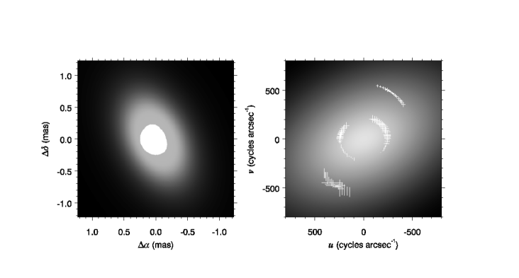
Figure 6: The disk model for $\gamma$ Cas. The left panel shows the appearance of the model star and disk in the sky (with the spin axis rotated east from north by angle $\alpha$). The right panel shows the associated Fourier transform of the spatial image, which is directly related to the predicted interferometric visibility. The plus signs in the upper half of the panel are scaled representations of the observed visibility squared at the $(u,v)$ coordinate of observation, while the mirror symmetric, thick line segments in the lower half show the scaled residuals from the fit (vertical for a positive residual and horizontal for a negative residual).

The star $\gamma$ Cas is perhaps the best documented Be star in the sky, and it has displayed Be, Be-shell, and normal B-type spectra over the course of the last century (Doazan, 1982). It currently displays strong H$\alpha$ emission, and the H$\alpha$ disk size was recently determined through observations from NPOI (Tycner et al., 2006). Our best fit disk (Table 6) and Gaussian elliptical models (Table 7) are generally consistent with the H$\alpha$ interferometric results and indicate that we view this Be star disk at an intermediate inclination. The disk density exponent we derive, $n=2.7\pm 0.3$, matches within errors the value $n=2.8\pm 0.1$ found by Hony et al. (2000) based on an analysis of the 2.4 – 45 $\mu$m spectrum from ISO-SWS. We show the model $K^{\prime}$ image of $\gamma$ Cas in the left hand panel of Figure 6 and the corresponding visibility image (without the effects of bandwidth smearing) is shown in the right hand panel. Both images are scaled logarithmic representations made to accentuate the low level features. The $(u,v)$ frequencies of the CHARA Array observations are shown in the upper half of the visibility image with symbol sizes proportional to the observed visibility. They also appear in point-symmetric locations in the lower half where they represent the residual-to-error ratio (vertical segment for $V_{\rm obs}>V_{\rm cal}$ and horizontal for $V_{\rm obs}<V_{\rm cal}$). The residuals from the fit are large for our observations of $\gamma$ Cas, but they do not appear to indicate any systematic deviation from the model since we find some of the largest positive and negative deviations in the same part of the $(u,v)$ diagram. We suspect that the high value of $\chi^{2}_{\nu}$ reflects an incomplete accounting of the full error budget.

Harmanec et al. (2000) discovered that $\gamma$ Cas is a single-lined spectroscopic binary, and their orbit was confirmed in subsequent Doppler shift measurements by Miroshnichenko et al. (2002). We made a fit of the visibilities by including a possible hot subdwarf companion that was placed in the model images using the spectroscopic ephemeris from Miroshnichenko et al. (2002) (Table 1). This modification made a slight improvement in the residuals of the fit, and models with a secondary hotter than $T_{\rm eff}=30$ kK showed somewhat better agreement.

The profiles of the H$\alpha$, H$\gamma$, and Br$\gamma$ emission lines are plotted as thick lines in Figure 7. We also plot the synthetic model profiles as thin lines for each feature. The model profiles of the weaker H$\gamma$ and Br$\gamma$ features make a reasonable match of the observed profiles, but, as noted above, the H$\alpha$ profile is much broader and smoother than predicted. Robinson, Smith, & Henry (2002) suggest that there may be significant turbulence in the inner disk of $\gamma$ Cas that is associated with magnetic dynamo processes, and such turbulent motions could help to explain the wings observed in H$\alpha$.

5.2 $\phi$ Per

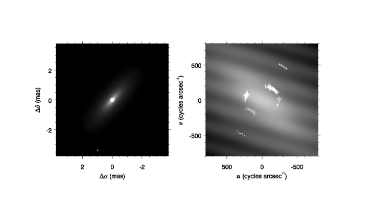
Figure 8: The model image and visibilities for the binary star fit of the interferometric data of $\phi$ Per in the same format as Fig. 6. The secondary appears as the bright dot in the lower part of the spatial image.

The binary system $\phi$ Per is the only one of the four targets where we known the nature of the secondary and can reliably predict its flux contribution in the near-IR (Gies et al., 1998). The companion is a hot subdwarf whose spectrum appears clearly in UV spectroscopy from HST, and from the relative strengths of its spectral lines, we can estimate with confidence its temperature, radius, and hence its near-IR flux contribution. Indeed the fit of the CHARA Array visibilities is better for the binary model than the single star model (Table 6). Here the inclusion of the binary flux leads to a downwards revision of the disk size. We show in left hand panel of Figure 8 the image of the entire binary for the observation made on HJD 2,453,656.9 (orbital phase 0.644), which is similar to the binary orientation for most of the observations (Table 4). The right hand panel shows the visibility image that is now modulated with the interference pattern introduced by the binary companion. Since the presence of the secondary does affect the visibility pattern, additional interferometric data should lead to an astrometric orbit that will allow us to test whether or not the disk and orbit are co-planar (Clarke & Bjorkman, 1998).

The position angle of the disk that we find is about $20^{\circ}$ different than that from the recent narrow-band H$\alpha$ measurements from Tycner et al. (2006) (Table 7). Our solution is somewhat influenced by our assumptions about the properties of the secondary’s orbit, and additional observations at other binary phases will be required to settle the issue of the disk and orbit orientations. We also find a much lower density exponent $n=1.8$ than the value of $n=3.0$ found by Waters et al. (1987) based on fitting the IR-excess from IRAS data, but their result is sensitive to the adopted disk radius. For example, Waters (1986) demonstrated that a density exponent of $n=2.4$ also fit the IR-excess provided the disk radius was limited to $R_{d}=6.5R_{\odot}$, so the difference in our results probably hinges on differences in the model assumptions.

Figure 9 shows the H$\alpha$, H$\gamma$, and Br$\gamma$ profiles for $\phi$ Per. The peaks in the H$\gamma$ profile reversed in strength between our observations in 2004 and 2005. This is an important reminder that the disk is time variable and is also probably somewhat asymmetrical in appearance (Hummel & Vrancken, 1995; Hummel & Štefl, 2001), properties that are beyond the scope of our simple disk models. Both the H$\alpha$ and Br$\gamma$ line are observed to be broader than predicted by the disk model.

5.3 $\zeta$ Tau

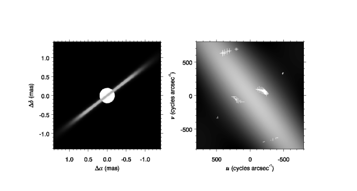
Figure 10: The model image and visibilities for the single star fit of the interferometric data of $\zeta$ Tau in the same format as Fig. 6.

Harmanec (1984) derived the best radial velocity curve to date for this single-lined binary, and we adopt his period here but we took the epoch from the the more recent spectroscopic study by Kaye & Gies (1997). A comparison of the single star and binary fits to the interferometry shows essentially no differences in the resulting $\chi^{2}_{\nu}$ values, so we will discuss the single star results here. The spatial and visibility images resulting from the fit are shown in Figure 10. Our results indicate that we are viewing this system close to edge-on, and the decline in visibility is especially marked along the direction of the projected major axis of the disk. Our derived orientation in the sky is in reasonable agreement with the H$\alpha$ results from Tycner et al. (2004), and the density law agrees within errors with that obtained from fitting the IR-excess flux (Waters et al., 1987).

The spectral line profiles of $\zeta$ Tau are illustrated in Figure 11. Again we find that the observed H$\alpha$ line is much broader than the model profile, and here we see evidence of a significant asymmetry in the disk in the differing heights of the blue and red emission peaks. The long term variations in these asymmetries are documented by Guo et al. (1995). Vakili et al. (1998) made H$\alpha$ interferometric observations in narrow bands matching the blue and red peaks, and their results support the idea that the disk density is modulated by a prograde one-armed oscillation. The H$\gamma$ line shows a deep central “shell” feature that is consistent with the formation of such shell lines in Be stars observed near $i=90^{\circ}$ (Hanuschik, 1996). The fact that our model H$\gamma$ line depth is shallower than the observed depth probably indicates that the outer parts of the disk are cooler than assumed in our isothermal model.

5.4 $\kappa$ Dra

Juza et al. (1991) and Saad et al. (2005) show that $\kappa$ Dra is a low amplitude, single-lined spectroscopic binary with a period of 65.6 d. Saad et al. (2004) describe a long-term cyclic variation of about 22 y that is present in the emission lines, and they suggest that this period may correspond to the disk’s modulation due to an interaction with a third star in an eccentric orbit. The semimajor axis of the third star would be on the order of 100 mas for the adopted distance, but we find no obvious evidence (separated fringe packets) for such a companion even at the shortest baselines. Thus, we have confined our test fits here to the single star and binary star ($P=65$ d) cases.

The fit for the single star case is odd in several respects. The density exponent is unusually small and the inclination of $i=90^{\circ}$ is at odds with estimates from spectroscopy ($i=35^{\circ}-45^{\circ}$; Juza et al. 1991). The binary fit has similar residuals, but it brings the density exponent and inclination into better accord with expectations. Thus, we will adopt the binary model that is based on a hot, subdwarf companion, but we caution that additional interferometric observations are required to make reliable estimates for the companion’s orbit and flux contribution.

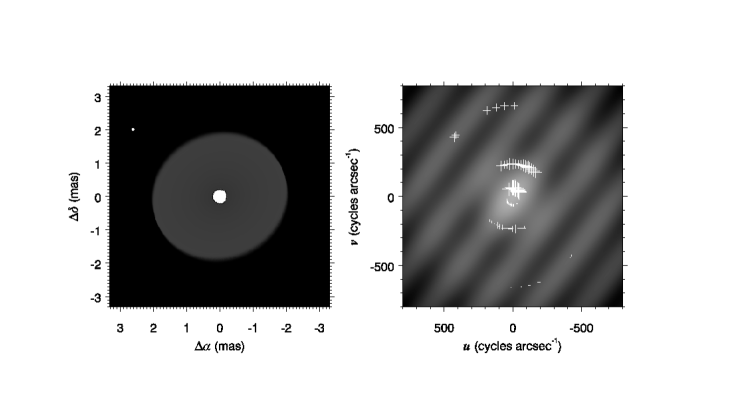
Figure 12: The model image and visibilities for the binary star fit of the interferometric data of $\kappa$ Dra in the same format as Fig. 6. The secondary appears as the bright dot in the upper left part of the spatial image.

The model spatial and visibility images are shown in Figure 12, and we see in this case that the binary modulation is equal to or greater than the disk variation in importance. The CHARA Array measurements presented here are the first interferometric observations of this target, so there are no H$\alpha$ results for comparison. Quirrenbach et al. (1997) found that the intrinsic continuum polarization angle is generally perpendicular to the projected disk major axis in the sky. Clarke (1990) estimated the intrinsic polarization angle for $\kappa$ Dra as $23^{\circ}$ east from north (in agreement with the estimate of $27^{\circ}$ from a recent polarization analysis by K. Bjorkman, private communication), and this agrees within errors with the position angle of $\alpha=21^{\circ}\pm 3^{\circ}$ from the fit of the interferometric visibilities.

The line profiles are shown in Figure 13. We find that the H$\alpha$ emission strength is approximately that expected for the epoch of our observations and the long term variation (see Fig. 4 of Saad et al. 2004). Once again the H$\alpha$ profile (and perhaps the H$\gamma$ profile) appear to be broader than predicted by the Keplerian model.

6 Conclusions

The CHARA Array observations represent the first $K^{\prime}$ interferometric measurements of northern Be stars, and we find that the disks of all four targets are at least partially resolved. The derived disk inclination angle and position angle in the sky generally agree with similar estimates from narrow-band H$\alpha$ interferometry where available. We find, for example, that the disk of $\zeta$ Tau appears with a nearly edge-on orientation, which is consistent with the prediction for Be stars with shell spectral features (Hanuschik, 1996). All four of the targets are close binaries with faint companions, and these companions appear to influence the $K^{\prime}$ visibilities of $\phi$ Per and $\kappa$ Dra, an interesting but complicating factor for the interpretation of the disk properties. We find, for example, that the radial gradient in disk density (density exponent $n$ in Table 6) is smaller in binaries with smaller semimajor axes, which suggests that binary companions do influence the disk properties.

We developed a simple Keplerian disk model to create synthetic angular images of the disks, and we used these models to create model interferometric visibility patterns and spectral emission line profiles for comparison with our observations. These models assume isothermal disks and ignore scattering in the radiative transfer process, two significant limitations that should be addressed in a more complete model. The disks are characterized by two physical parameters, the base density and density exponent, and two observational parameters, the disk normal inclination and position angle. We fit the CHARA Array visibilities for all four parameters for both single and binary star models, and our results are in good agreement with prior studies of the IR-excess in these stars. The parameters derived from the interferometry lead to model emission lines that match the observed ones if the base densities are reduced by a factor of about 1.7 dex. This mismatch is not unexpected considering the many simplifying assumptions made in the model.

We find that the angular diameters of the Be disks in the $K^{\prime}$-band are consistently smaller than those found from H$\alpha$ interferometry. We think that this difference results from the larger H$\alpha$ opacity and the hydrogen ionization structure in the disk. The $K^{\prime}$ disk emission comes primarily from free-free processes in the mainly ionized gas, and the free-free optical depth will vary with disk radius according to the square of the density. In the thin disk approximation, the optical depth at radial distance $R$ will vary as $\tau\propto\rho_{0}^{2}~{}R^{-2n+3/2}/\cos i$ (see eq. [2] and [3]). On the other hand, the H$\alpha$ emission depends on the relatively low neutral hydrogen number density, and we assumed above that this varies inversely with the stellar dilution factor (eq. [9]; $W(r)\propto R^{-2}$ at large radius and $Z=0$). Thus, we expect the H$\alpha$ optical depth to vary approximately as $\tau\propto\rho_{0}^{2}~{}R^{-2n+3/2+2}/\cos i$, i.e., with a shallower effective density exponent of $n-1$. Consequently, the H$\alpha$ optical depth reduction with increasing disk radius will be less pronounced than in the case of the IR optical depth, resulting in a larger spatial extension in the H$\alpha$ emission compared to that for the $K^{\prime}$ emission.

This expectation is borne out in the predicted spatial images. We show an example of the derived spatial structure in Figure 14 for our single star model of $\gamma$ Cas. The solid line shows the summed $K^{\prime}$-band intensity of the image projected onto the major axis of the disk and measured in stellar radii from the center of the star. We used our model to create an H$\alpha$ image adopting the base density from the fit of the observed emission line (Table 8). The intensity was formed by summing across a 2.8 nm wavelength band centered on H$\alpha$ in order to match the H$\alpha$ interferometric observations of Tycner et al. (2006). Note that changing the adopted bandwidth will simply result in a rescaling of the contrast between the central star and the surrounding disk emission. The disk image appears darker along the line of nodes and along the line of sight because of the minimal shear broadening that occurs at those disk azimuthal angles and the subsequent reduction in the range of wavelength over which H$\alpha$ is optically thick. The dashed line in Figure 14 shows the summed H$\alpha$ image intensity projected onto the major axis. We see that H$\alpha$ emission is indeed more extended along the major axis and that the half maximum intensity radii are located at $2.6R_{\star}$ and $7.4R_{\star}$ for the $K^{\prime}$ band and H$\alpha$ summed intensities, respectively. The ratio of these half maximum intensity radii is 0.35, which is comparable to the observed ratio of 0.55 of the FWHM of the major axes of the $K^{\prime}$-band and H$\alpha$ emission in the Gaussian elliptical fits (Table 7). Thus, the differences in the radial exponent dependence of density squared and the neutral hydrogen fraction may partially explain the larger appearance of the H$\alpha$ disks.

The CHARA Array observations demonstrate the promise of these kinds of measurements for our understanding of Be stars. Many Be stars were probably spun up by mass transfer in a past close interaction, and future observations over a range in $(u,v)$ and orbital phase coverage will reveal the nature of their companions. The disks of Be stars are driven by dynamic processes and evolve over timescales of months to years, so long-term observations will help elucidate the physics of disk formation and dispersal. There is ample evidence that the disks are structured and prone to the formation of spiral arm features (Okazaki et al., 2002). Furthermore, in Be binaries like $\phi$ Per, the portion of the disk closest to the hot companion may appear brighter due to local heating by the companion’s radiation (Gies et al., 1998; Hummel & Štefl, 2001). The techniques of phase closure using multiple telescopes in long baseline interferometry (Kraus et al., 2005) will soon give us the means to study these disk processes directly among the nearby Be stars.

Table 1: Adopted Stellar Parameters

Parameter	$\gamma$ Cas	$\phi$ Per	$\zeta$ Tau	$\kappa$ Dra
Spectral Classification	B0.5 Ve	B0.5 III-Ve	B2 IIIpe	B5-6 IIIe
$\pi$ (mas)	5.32	4.55	7.82	6.55
$R_{1}$ ($R_{\odot}$)	10.0	7.0	5.5	6.4
$M_{1}$ ($M_{\odot}$)	15.5	9.3	11.2	4.8
$T_{1~{}\rm eff}$ (K)	28840	29300	19000	14000
$V\sin i$ (km s-1)	295	410	320	170
$R_{2}$ ($R_{\odot}$)	1.0	1.33	1.0	1.0
$M_{2}$ ($M_{\odot}$)	1.0	1.1	1.0	0.8
$T_{2~{}\rm eff}$ (K)	30000	53000	30000	30000
$P$ (d)	203.59	126.67	132.91	61.56
$T_{S+}$ (HJD–2,400,000)	50654.3	50155.1	46417.3	50011.0
$a_{1}\sin i$ ($R_{\odot}$)	15.279	24.942	27.562	10.078
$R_{d}$ ($R_{\odot}$)	214	130	146	67
References	1, 2	3	4, 5, 6	7

References. — 1. Harmanec et al. (2000); 2. Miroshnichenko et al. (2002); 3. Gies et al. (1998); 4. Harmanec (1984); 5. Yang et al. (1990); 6. Kaye & Gies (1997); 7. Saad et al. (2005).

Table 2: CHARA Array Observations

Target	Calibrator	Baseline	Date	No. of
Name	Name	(m)	(UT)	Sets
$\gamma$ Cas	HD 6210	W1/S2 (249)	2003 Oct 07	05
$\gamma$ Cas	HD 6210	W1/S2 (249)	2003 Oct 10	06
$\gamma$ Cas	HD 6210	W1/S2 (249)	2003 Oct 14	05
$\gamma$ Cas	HD 6210	W1/S2 (249)	2003 Oct 16	06
$\gamma$ Cas	HD 6210	W1/W2 (111)	2005 Oct 12	12
$\gamma$ Cas	HD 6210	W1/W2 (111)	2005 Oct 13	11
$\gamma$ Cas	HD 6210	W1/W2 (111)	2005 Oct 15	11
$\phi$ Per	HD 6961	W1/S2 (249)	2003 Oct 03	05
$\phi$ Per	HD 6961	W1/W2 (111)	2003 Oct 12	10
$\phi$ Per	HD 6961	W1/W2 (111)	2003 Oct 13	07
$\phi$ Per	HD 6961	W1/W2 (111)	2003 Oct 14	14
$\zeta$ Tau	HD 43042	S1/E1 (331)	2004 Dec 21	06
$\zeta$ Tau	HD 32977	S1/E1 (331)	2004 Dec 22	01
$\zeta$ Tau	HD 43042	W1/S1 (279)	2005 Apr 01	02
$\zeta$ Tau	HD 43042	W1/W2 (111)	2005 Dec 04	08
$\zeta$ Tau	HD 43042	W1/W2 (111)	2005 Dec 05	09
$\kappa$ Dra	HD 107193	S1/S2 (34)0	2005 Apr 02	13
$\kappa$ Dra	HD 107193	S1/E1 (331)	2005 Apr 06	05
$\kappa$ Dra	HD 107193	S1/E1 (331)	2005 Apr 13	01
$\kappa$ Dra	HD 107193	W1/W2 (111)	2005 Dec 04	03
$\kappa$ Dra	HD 107193	W1/W2 (111)	2005 Dec 05	13

Table 3: Calibrator Star Angular Diameters

Calibrator	$T_{\rm eff}$	$\log g$	Spectral	$E(B-V)$	$\theta_{LD}$
Name	(K)	(cm s-2)	Classification	(mag)	(mas)	Ref.
HD 6210	6087	3.73	F6 V	0.00	$0.523\pm 0.027$	1, 2, 3, 4
HD 6961	7762	3.80	A7 V var	0.00	$0.608\pm 0.019$	2
HD 32977	8511	4.19	A5 V	0.00	$0.344\pm 0.033$	2
HD 43042	6556	4.28	F6 V	0.00	$0.590\pm 0.016$	3
HD 107193	8710	3.93	A0 Vn	0.04	$0.308\pm 0.005$	2

References. — 1. Cayrel de Strobel et al. (1997); 2. Allende Prieto & Lambert (1999); 3. Lambert & Reddy (2004); 4. Nordström et al. (2004).

Table 4: Calibrated $K^{\prime}$ Visibilities

Target	Date	Orbital	Telescope	Baseline	Pos. Ang.
Name	(HJD-2,400,000)	Phase	Pair	(m)	(deg)	Visibility
$\gamma$ Cas	52919.721	0.127	W1/S2	247.37	345.28	$0.445\pm 0.016$
$\gamma$ Cas	52919.731	0.127	W1/S2	247.09	342.34	$0.448\pm 0.016$
$\gamma$ Cas	52919.742	0.127	W1/S2	246.71	339.22	$0.490\pm 0.017$
$\gamma$ Cas	52919.751	0.128	W1/S2	246.28	336.45	$0.516\pm 0.017$
$\gamma$ Cas	52919.759	0.128	W1/S2	245.87	334.14	$0.608\pm 0.019$
$\gamma$ Cas	52922.794	0.142	W1/S2	242.31	321.83	$0.496\pm 0.016$
$\gamma$ Cas	52922.804	0.143	W1/S2	241.12	319.06	$0.522\pm 0.016$
$\gamma$ Cas	52922.812	0.143	W1/S2	240.06	316.88	$0.595\pm 0.015$
$\gamma$ Cas	52922.819	0.143	W1/S2	239.06	315.01	$0.593\pm 0.018$
$\gamma$ Cas	52922.825	0.143	W1/S2	238.11	313.36	$0.592\pm 0.024$
$\gamma$ Cas	52922.834	0.143	W1/S2	236.47	310.77	$0.624\pm 0.018$
$\gamma$ Cas	52926.747	0.162	W1/S2	245.49	332.32	$0.458\pm 0.019$
$\gamma$ Cas	52926.754	0.162	W1/S2	244.98	330.14	$0.381\pm 0.014$
$\gamma$ Cas	52926.763	0.162	W1/S2	244.28	327.54	$0.424\pm 0.018$
$\gamma$ Cas	52926.770	0.162	W1/S2	243.70	325.68	$0.509\pm 0.016$
$\gamma$ Cas	52926.777	0.162	W1/S2	243.05	323.78	$0.533\pm 0.018$
$\gamma$ Cas	52928.731	0.172	W1/S2	246.08	335.28	$0.281\pm 0.026$
$\gamma$ Cas	52928.740	0.172	W1/S2	245.57	332.66	$0.266\pm 0.023$
$\gamma$ Cas	52928.746	0.172	W1/S2	245.20	331.04	$0.313\pm 0.016$
$\gamma$ Cas	52928.753	0.172	W1/S2	244.64	328.83	$0.287\pm 0.010$
$\gamma$ Cas	52928.761	0.172	W1/S2	244.00	326.62	$0.298\pm 0.011$
$\gamma$ Cas	52928.770	0.172	W1/S2	243.21	324.23	$0.303\pm 0.009$
$\gamma$ Cas	53655.813	0.743	W1/W2	107.91	100.65	$0.826\pm 0.019$
$\gamma$ Cas	53655.826	0.743	W1/W2	107.91	096.49	$0.790\pm 0.018$
$\gamma$ Cas	53655.842	0.743	W1/W2	107.70	091.62	$0.791\pm 0.021$
$\gamma$ Cas	53655.854	0.743	W1/W2	107.34	087.65	$0.816\pm 0.019$
$\gamma$ Cas	53655.866	0.743	W1/W2	106.84	083.78	$0.807\pm 0.019$
$\gamma$ Cas	53655.879	0.743	W1/W2	106.19	079.89	$0.756\pm 0.019$
$\gamma$ Cas	53655.891	0.743	W1/W2	105.37	075.74	$0.781\pm 0.017$
$\gamma$ Cas	53655.904	0.743	W1/W2	104.45	071.72	$0.777\pm 0.017$
$\gamma$ Cas	53655.916	0.743	W1/W2	103.41	067.63	$0.779\pm 0.018$
$\gamma$ Cas	53655.929	0.744	W1/W2	102.19	063.12	$0.782\pm 0.019$
$\gamma$ Cas	53655.942	0.744	W1/W2	100.93	058.68	$0.735\pm 0.018$
$\gamma$ Cas	53655.961	0.744	W1/W2	099.00	052.04	$0.741\pm 0.021$
$\gamma$ Cas	53656.652	0.747	W1/W2	099.51	155.13	$0.839\pm 0.024$
$\gamma$ Cas	53656.664	0.747	W1/W2	100.24	150.39	$0.809\pm 0.023$
$\gamma$ Cas	53656.678	0.747	W1/W2	101.09	145.40	$0.830\pm 0.029$
$\gamma$ Cas	53656.691	0.747	W1/W2	101.97	140.64	$0.792\pm 0.027$
$\gamma$ Cas	53656.707	0.747	W1/W2	103.12	134.75	$0.829\pm 0.032$
$\gamma$ Cas	53656.720	0.747	W1/W2	104.04	130.07	$0.833\pm 0.024$
$\gamma$ Cas	53656.734	0.747	W1/W2	104.90	125.58	$0.859\pm 0.021$
$\gamma$ Cas	53656.747	0.748	W1/W2	105.70	121.17	$0.833\pm 0.021$
$\gamma$ Cas	53656.762	0.748	W1/W2	106.52	116.04	$0.878\pm 0.022$
$\gamma$ Cas	53656.775	0.748	W1/W2	107.10	111.71	$0.840\pm 0.020$
$\gamma$ Cas	53656.788	0.748	W1/W2	107.51	107.71	$0.884\pm 0.025$
$\gamma$ Cas	53658.701	0.757	W1/W2	103.11	134.83	$0.875\pm 0.021$
$\gamma$ Cas	53658.714	0.757	W1/W2	103.97	130.47	$0.830\pm 0.020$
$\gamma$ Cas	53658.727	0.757	W1/W2	104.86	125.83	$0.851\pm 0.018$
$\gamma$ Cas	53658.741	0.757	W1/W2	105.67	121.35	$0.878\pm 0.019$
$\gamma$ Cas	53658.814	0.758	W1/W2	107.93	097.77	$0.779\pm 0.021$
$\gamma$ Cas	53658.827	0.758	W1/W2	107.82	093.74	$0.742\pm 0.021$
$\gamma$ Cas	53658.840	0.758	W1/W2	107.54	089.60	$0.740\pm 0.023$
$\gamma$ Cas	53658.854	0.758	W1/W2	107.01	084.98	$0.704\pm 0.024$
$\gamma$ Cas	53658.876	0.758	W1/W2	105.88	078.23	$0.684\pm 0.022$
$\gamma$ Cas	53658.892	0.758	W1/W2	104.77	073.07	$0.740\pm 0.022$
$\gamma$ Cas	53658.906	0.758	W1/W2	103.61	068.38	$0.754\pm 0.025$
$\phi$ Per	52915.807	0.794	W1/S2	249.35	333.52	$0.533\pm 0.019$
$\phi$ Per	52915.818	0.794	W1/S2	249.21	330.46	$0.520\pm 0.016$
$\phi$ Per	52915.829	0.794	W1/S2	248.93	327.43	$0.475\pm 0.015$
$\phi$ Per	52915.840	0.794	W1/S2	248.50	324.62	$0.540\pm 0.016$
$\phi$ Per	52915.850	0.794	W1/S2	247.94	322.06	$0.586\pm 0.020$
$\phi$ Per	53655.657	0.635	W1/W2	089.21	165.54	$0.771\pm 0.028$
$\phi$ Per	53655.673	0.635	W1/W2	090.30	159.13	$0.753\pm 0.022$
$\phi$ Per	53655.687	0.635	W1/W2	091.70	153.00	$0.783\pm 0.027$
$\phi$ Per	53655.702	0.635	W1/W2	093.31	147.18	$0.743\pm 0.020$
$\phi$ Per	53655.715	0.635	W1/W2	094.94	142.08	$0.789\pm 0.021$
$\phi$ Per	53655.728	0.635	W1/W2	096.63	137.21	$0.724\pm 0.019$
$\phi$ Per	53655.743	0.635	W1/W2	098.54	132.02	$0.749\pm 0.020$
$\phi$ Per	53655.758	0.635	W1/W2	100.43	127.03	$0.753\pm 0.018$
$\phi$ Per	53655.772	0.635	W1/W2	102.16	122.38	$0.761\pm 0.019$
$\phi$ Per	53655.789	0.636	W1/W2	104.03	117.05	$0.724\pm 0.018$
$\phi$ Per	53656.864	0.644	W1/W2	107.89	094.57	$0.836\pm 0.025$
$\phi$ Per	53656.878	0.644	W1/W2	107.55	090.58	$0.866\pm 0.024$
$\phi$ Per	53656.892	0.644	W1/W2	106.92	086.85	$0.840\pm 0.024$
$\phi$ Per	53656.905	0.644	W1/W2	106.00	083.15	$0.827\pm 0.024$
$\phi$ Per	53656.932	0.645	W1/W2	103.25	075.29	$0.820\pm 0.031$
$\phi$ Per	53656.947	0.645	W1/W2	101.27	070.73	$0.875\pm 0.026$
$\phi$ Per	53656.960	0.645	W1/W2	099.35	066.67	$0.887\pm 0.026$
$\phi$ Per	53657.690	0.651	W1/W2	092.54	149.83	$0.937\pm 0.039$
$\phi$ Per	53657.703	0.651	W1/W2	094.10	144.64	$0.880\pm 0.031$
$\phi$ Per	53657.717	0.651	W1/W2	095.89	139.29	$0.744\pm 0.024$
$\phi$ Per	53657.733	0.651	W1/W2	097.90	133.73	$0.684\pm 0.022$
$\phi$ Per	53657.746	0.651	W1/W2	099.59	129.25	$0.643\pm 0.021$
$\phi$ Per	53657.759	0.651	W1/W2	101.25	124.84	$0.554\pm 0.018$
$\phi$ Per	53657.775	0.651	W1/W2	103.18	119.53	$0.620\pm 0.018$
$\phi$ Per	53657.790	0.651	W1/W2	104.65	115.13	$0.707\pm 0.021$
$\phi$ Per	53657.879	0.652	W1/W2	107.40	089.50	$0.725\pm 0.027$
$\phi$ Per	53657.892	0.652	W1/W2	106.71	085.92	$0.826\pm 0.020$
$\phi$ Per	53657.905	0.652	W1/W2	105.77	082.34	$0.861\pm 0.021$
$\phi$ Per	53657.925	0.652	W1/W2	103.73	076.48	$0.924\pm 0.017$
$\phi$ Per	53657.938	0.653	W1/W2	102.16	072.72	$0.931\pm 0.016$
$\phi$ Per	53657.950	0.653	W1/W2	100.36	068.77	$0.939\pm 0.016$
$\zeta$ Tau	53360.760	0.242	S1/E1	329.84	033.00	$0.924\pm 0.037$
$\zeta$ Tau	53360.774	0.242	S1/E1	328.55	030.86	$0.918\pm 0.034$
$\zeta$ Tau	53360.795	0.242	S1/E1	325.81	027.32	$0.898\pm 0.036$
$\zeta$ Tau	53360.807	0.242	S1/E1	323.78	024.94	$0.789\pm 0.038$
$\zeta$ Tau	53360.845	0.242	S1/E1	317.39	017.02	$0.615\pm 0.021$
$\zeta$ Tau	53360.850	0.242	S1/E1	316.65	015.94	$0.609\pm 0.020$
$\zeta$ Tau	53361.760	0.249	S1/E1	329.62	032.58	$0.813\pm 0.038$
$\zeta$ Tau	53461.662	0.001	W1/S1	261.82	304.56	$0.368\pm 0.019$
$\zeta$ Tau	53461.673	0.001	W1/S1	256.24	303.94	$0.438\pm 0.019$
$\zeta$ Tau	53708.795	0.860	W1/W2	092.98	108.47	$0.748\pm 0.024$
$\zeta$ Tau	53708.809	0.860	W1/W2	096.78	106.04	$0.719\pm 0.023$
$\zeta$ Tau	53708.822	0.860	W1/W2	100.05	103.84	$0.803\pm 0.022$
$\zeta$ Tau	53708.838	0.861	W1/W2	103.33	101.35	$0.775\pm 0.028$
$\zeta$ Tau	53708.853	0.861	W1/W2	105.68	099.12	$0.746\pm 0.022$
$\zeta$ Tau	53708.869	0.861	W1/W2	107.24	096.97	$0.767\pm 0.022$
$\zeta$ Tau	53708.876	0.861	W1/W2	107.67	095.97	$0.716\pm 0.021$
$\zeta$ Tau	53708.890	0.861	W1/W2	107.93	094.14	$0.675\pm 0.020$
$\zeta$ Tau	53709.718	0.867	W1/W2	065.27	129.49	$0.742\pm 0.032$
$\zeta$ Tau	53709.734	0.867	W1/W2	071.89	123.24	$0.924\pm 0.029$
$\zeta$ Tau	53709.751	0.867	W1/W2	078.20	118.27	$0.868\pm 0.028$
$\zeta$ Tau	53709.765	0.868	W1/W2	083.77	114.39	$0.946\pm 0.029$
$\zeta$ Tau	53709.782	0.868	W1/W2	089.40	110.74	$0.927\pm 0.028$
$\zeta$ Tau	53709.795	0.868	W1/W2	093.81	107.95	$0.948\pm 0.032$
$\zeta$ Tau	53709.809	0.868	W1/W2	097.51	105.57	$0.815\pm 0.021$
$\zeta$ Tau	53709.823	0.868	W1/W2	100.87	103.25	$0.803\pm 0.029$
$\zeta$ Tau	53709.840	0.868	W1/W2	104.15	100.64	$0.720\pm 0.019$
$\kappa$ Dra	53462.655	0.074	S1/S2	026.40	029.89	$0.929\pm 0.037$
$\kappa$ Dra	53462.756	0.076	S1/S2	027.74	004.61	$0.995\pm 0.021$
$\kappa$ Dra	53462.774	0.076	S1/S2	027.77	000.27	$0.997\pm 0.022$
$\kappa$ Dra	53462.801	0.077	S1/S2	027.70	353.51	$1.002\pm 0.025$
$\kappa$ Dra	53462.827	0.077	S1/S2	027.51	346.82	$1.058\pm 0.041$
$\kappa$ Dra	53462.845	0.077	S1/S2	027.29	342.31	$0.990\pm 0.023$
$\kappa$ Dra	53462.859	0.078	S1/S2	027.09	338.86	$1.019\pm 0.034$
$\kappa$ Dra	53462.909	0.078	S1/S2	026.04	326.47	$1.018\pm 0.028$
$\kappa$ Dra	53462.926	0.079	S1/S2	025.55	322.13	$0.974\pm 0.035$
$\kappa$ Dra	53462.946	0.079	S1/S2	024.92	317.18	$1.027\pm 0.025$
$\kappa$ Dra	53462.963	0.079	S1/S2	024.27	312.66	$0.979\pm 0.021$
$\kappa$ Dra	53462.982	0.080	S1/S2	023.50	307.78	$1.045\pm 0.024$
$\kappa$ Dra	53462.999	0.080	S1/S2	022.79	303.56	$0.999\pm 0.042$
$\kappa$ Dra	53466.750	0.141	S1/E1	267.57	043.26	$0.686\pm 0.022$
$\kappa$ Dra	53466.847	0.142	S1/E1	286.48	016.95	$0.738\pm 0.032$
$\kappa$ Dra	53466.870	0.143	S1/E1	288.46	010.67	$0.727\pm 0.032$
$\kappa$ Dra	53466.890	0.143	S1/E1	289.41	005.37	$0.714\pm 0.031$
$\kappa$ Dra	53466.914	0.144	S1/E1	289.72	358.90	$0.681\pm 0.033$
$\kappa$ Dra	53473.724	0.254	S1/E1	265.84	044.86	$0.776\pm 0.029$
$\kappa$ Dra	53708.995	0.076	W1/W2	104.62	154.45	$0.832\pm 0.027$
$\kappa$ Dra	53709.008	0.077	W1/W2	104.95	149.84	$0.855\pm 0.057$
$\kappa$ Dra	53709.020	0.077	W1/W2	105.29	145.59	$0.847\pm 0.055$
$\kappa$ Dra	53709.868	0.090	W1/W2	104.32	200.84	$0.817\pm 0.026$
$\kappa$ Dra	53709.883	0.091	W1/W2	104.05	195.44	$0.713\pm 0.018$
$\kappa$ Dra	53709.897	0.091	W1/W2	103.85	190.28	$0.753\pm 0.023$
$\kappa$ Dra	53709.910	0.091	W1/W2	103.73	185.24	$0.859\pm 0.021$
$\kappa$ Dra	53709.925	0.091	W1/W2	103.69	179.64	$0.835\pm 0.018$
$\kappa$ Dra	53709.937	0.092	W1/W2	103.73	175.03	$0.760\pm 0.017$
$\kappa$ Dra	53709.950	0.092	W1/W2	103.83	170.33	$0.719\pm 0.015$
$\kappa$ Dra	53709.962	0.092	W1/W2	104.00	165.71	$0.799\pm 0.018$
$\kappa$ Dra	53709.975	0.092	W1/W2	104.21	161.15	$0.873\pm 0.015$
$\kappa$ Dra	53709.987	0.092	W1/W2	104.48	156.65	$0.889\pm 0.018$
$\kappa$ Dra	53710.000	0.093	W1/W2	104.80	151.94	$0.926\pm 0.022$
$\kappa$ Dra	53710.031	0.093	W1/W2	105.70	140.57	$0.879\pm 0.026$
$\kappa$ Dra	53710.043	0.093	W1/W2	106.07	136.19	$0.871\pm 0.029$

Table 5: Spectroscopic Observations

		Resolving	Range	Date
Telescope	Spectrograph	Power	(Å)	(UT)	Targets
KPNO coudé feed 0.9 m	Coude	12800	4235–4586	2004 Aug 16–21	$\gamma$ Cas, $\phi$ Per
KPNO coudé feed 0.9 m	Coude	12800	4236–4587	2005 Nov 10–14	$\gamma$ Cas, $\phi$ Per, $\zeta$ Tau, $\kappa$ Dra
KPNO coudé feed 0.9 m	Coude	09150	6465–7140	2004 Oct 12–14	$\gamma$ Cas, $\phi$ Per, $\zeta$ Tau
McDonald Obs. 2.7 m	CoolSpec	01520	20691–22520	2004 Feb 06	$\gamma$ Cas, $\phi$ Per, $\zeta$ Tau
McDonald Obs. 2.7 m	LCS	00810	3020–5717	2005 Apr 29	$\kappa$ Dra
Ondřejov Obs. 2.0 m	Coude	12800	6262–6774	2005 Apr 11	$\kappa$ Dra
Ritter Obs. 1.0 m	Echelle	26000	5413–6596	2005 Apr 10	$\kappa$ Dra

Table 6: Thick Disk Model Fits of Visibilities

	$\gamma$ Cas	$\gamma$ Cas	$\phi$ Per	$\phi$ Per	$\zeta$ Tau	$\zeta$ Tau	$\kappa$ Dra	$\kappa$ Dra
Parameter	Single	Binary	Single	Binary	Single	Binary	Single	Binary
$i$ (deg)	$51\pm 4$	$127\pm 4$	$90\pm 7$	$69\pm 5$	$90\pm 3$	$89\pm 2$	$72\pm 18$	$26\pm 9$
$\alpha$ (deg)	$116\pm 4$	$114\pm 3$	$46\pm 4$	$49\pm 3$	$38\pm 2$	$37\pm 2$	$114\pm 4$	$21\pm 3$
$\log\rho_{0~{}{\rm fit}}$ (g cm-3)	$-10.14\pm 0.24$	$-10.18\pm 0.25$	$-10.92\pm 0.10$	$-10.98\pm 0.08$	$-9.71\pm 0.31$	$-9.73\pm 0.35$	$-12.55\pm 0.39$	$-12.21\pm 0.32$
$\log\rho_{0~{}{\rm IRAS}}$ (g cm-3)	$-10.95\pm 0.35$	$-10.95\pm 0.35$	$-10.85\pm 0.25$	$-10.85\pm 0.25$	$-11.15\pm 0.25$	$-11.15\pm 0.25$	$-11.35\pm 0.15$	$-11.35\pm 0.15$
$n_{\rm fit}$	$2.70\pm 0.31$	$2.65\pm 0.32$	$1.80\pm 0.09$	$1.76\pm 0.08$	$3.14\pm 0.38$	$3.19\pm 0.40$	$0.16\pm 0.43$	$0.67\pm 0.36$
$n_{\rm IRAS}$	3.25	3.25	3.0	3.0	3.25	3.25	3.0	3.0
$\chi^{2}_{\nu}$	24.3	24.0	8.0	7.1	7.9	7.9	4.0	4.0
$E(V-K)_{\rm fit}$ (mag)	1.60	1.53	0.58	0.63	0.53	0.40	0.31	0.14
$E(V-K)_{\rm obs}$ (mag)	0.85	0.85	0.68	0.68	0.65	0.65	0.39	0.39
$\theta_{LD}$ (mas)	0.50	0.50	0.30	0.30	0.40	0.40	0.39	0.39
Disk FWHM (mas)	1.35	1.36	0.98	0.51	1.99	1.82	3.02	1.72

Table 7: Gaussian Elliptical Fits of Visibilities

Parameter	$\gamma$ Cas	$\phi$ Per	$\zeta$ Tau	$\kappa$ Dra
$\theta_{\rm GD~{}fit}$ (mas)	$1.95\pm 0.07$	$2.30\pm 0.08$	$1.79\pm 0.07$	$1.83\pm 0.11$
$\theta_{{\rm GD~{}H}\alpha}$ (mas)	$3.47\pm 0.02$	$2.67\pm 0.20$	$4.53\pm 0.52$	$\cdots$
$\theta_{{\rm GD~{}H}\alpha}$ (mas)	$3.59\pm 0.04$	$2.89\pm 0.09$	$3.14\pm 0.21$	$\cdots$
$r_{\rm fit}$	$0.59\pm 0.04$	$0.00\pm 0.22$	$0.09\pm 0.22$	$0.00\pm 0.67$
$r_{{\rm H}\alpha}$	$0.70\pm 0.02$	$0.46\pm 0.04$	$0.28\pm 0.02$	$\cdots$
$r_{{\rm H}\alpha}$	$0.58\pm 0.03$	$0.27\pm 0.01$	$0.31\pm 0.07$	$\cdots$
$\phi_{\rm fit}$ (deg)	$25\pm 4$	$-44\pm 3$	$-52.2\pm 1.7$	$-8\pm 9$
$\phi_{{\rm H}\alpha}$ (deg)	$19\pm 2$	$-62\pm 5$	$-58\pm 4$	$\cdots$
$\phi_{{\rm H}\alpha}$ (deg)	$31.2\pm 1.2$	$-61.5\pm 0.6$	$-62.3\pm 4.4$	$\cdots$
$c_{\rm P~{}fit}$	$0.395\pm 0.018$	$0.538\pm 0.015$	$0.414\pm 0.029$	$0.628\pm 0.030$
$\chi^{2}_{\nu}$	23.6	7.9	7.7	8.6

Table 8: Emission Line Equivalent Widths and Density Fits

Parameter	$\gamma$ Cas	$\phi$ Per	$\zeta$ Tau	$\kappa$ Dra
$W_{\lambda}({\rm H}\alpha)$ (Å)	$-31.2$	$-42.6$	$-19.5$	$-20.3$
$W_{\lambda}({\rm H}\gamma)$ (Å)	0$+1.0$	0$+2.1$	0$+4.0$	0$+5.9$
$W_{\lambda}({\rm Br}\gamma)$ (Å)	0$-5.8$	0$-9.2$	0$-2.8$	$\cdots$
$\log\rho_{0~{}{\rm fit}}({\rm H}\alpha)$ (g cm-3)	$-11.7$	$-12.5$	$-11.2$	$-13.4$
$\log\rho_{0~{}{\rm fit}}({\rm H}\gamma)$ (g cm-3)	$-11.7$	$-12.8$	$-11.2$	$-13.7$
$\log\rho_{0~{}{\rm fit}}({\rm Br}\gamma)$ (g cm-3)	$-12.0$	$-12.9$	$-11.7$	$\cdots$
$\log\rho_{0~{}{\rm fit}}(K^{\prime})$ (g cm-3)	$-10.1\pm 0.2$	$-11.0\pm 0.1$	$-9.7\pm 0.3$	$-12.2\pm 0.3$

Figure 5: The observed H$\alpha$ line in $\gamma$ Cas (thick line) compared with the synthetic profile for a Keplerian disk (double-peaked thin line) and the same convolved with a Voigt profile (broader thin line).

Figure 7: Hydrogen line profiles in the spectrum of $\gamma$ Cas plotted as a function of heliocentric radial velocity. The solid, thick lines indicate spectra made in 2004 while the dashed, thick lines correspond to 2005 observations. The thin lines represent the model synthetic spectra. The continuum levels for H$\alpha$ (top) and H$\gamma$ (middle) are offset in rectified flux by $+2$ and $+1$, respectively, for clarity of presentation.

Figure 9: Hydrogen line profiles in the spectrum of $\phi$ Per plotted in the same format as Fig. 7.

Figure 11: Hydrogen line profiles in the spectrum of $\zeta$ Tau plotted in the same format as Fig. 7, except that the Br$\gamma$ profile is offset by $-0.5$ in flux for clarity.

Figure 13: Hydrogen line profiles in the spectrum of $\kappa$ Dra plotted in the same format as Fig. 7. We lack observations of Br$\gamma$ for this star but we include our low resolution spectrum of H$\beta$ instead (without a synthetic comparison). The continuum levels for H$\alpha$ (top) and H$\beta$ (middle) are offset in rectified flux by $+2$ and $+1$, respectively, for clarity of presentation.

Figure 14: The summed spatial intensities projected onto the major axis for our single star model of $\gamma$ Cas. The solid line shows the $K^{\prime}$-band summed intensity while the dashed line shows the summed intensity for an H$\alpha$ image integrated over a 2.8 nm bandwidth. Both are renormalized for convenience to their respective summed intensity at $R=1.14R_{\star}$.

References

- Abt et al. (2002) Abt, H. A, Levato, H., & Grosso, M. 2002, ApJ, 573, 359
- Allende Prieto & Lambert (1999) Allende Prieto, C., & Lambert, D. L. 1999, A&A, 352, 555
- Aufdenberg et al. (2006) Aufdenberg, J. P., et al. 2006, ApJ, 645, 664
- Berger et al. (2006) Berger, D. H., et al. 2006, ApJ, 644, 475
- Berio et al. (1999) Berio, P., et al. 1999, A&A, 345, 203
- Bjorkman & Bjorkman (1994) Bjorkman, J. E., & Bjorkman, K. S. 1994, ApJ, 436, 818
- Carciofi & Bjorkman (2006) Carciofi, A. C., & Bjorkman, J. E. 2006, ApJ, 639, 1081
- Cassinelli et al. (1987) Cassinelli, J. P., Nordsieck, K. H., & Murison, M. A. 1987, ApJ, 317, 290
- Cayrel de Strobel et al. (1997) Cayrel de Strobel, G., Soubiran, C., Friel, E. D., Ralite, N., & Francois, P. 1997, A&A, 124, 299
- Chesneau et al. (2005) Chesneau, O., et al. 2005, A&A, 435, 275
- Claret (2000) Claret, A. 2000, A&A, 363, 1081
- Clarke (1990) Clarke, D. 1990, A&A, 227, 151
- Clarke & Bjorkman (1998) Clarke, D., & Bjorkman, K. S. 1998, A&A, 331, 1059
- Cohen et al. (2003) Cohen, M., Wheaton, W. A., & Megeath, S. T. 2003, AJ, 126, 1090
- Colina et al. (1996) Colina, L., Bohlin, R., & Castelli, F. 1996, HST Instrument Science Report CAL/SCS-008 (Baltimore: STScI)
- Coté & Waters (1987) Coté, J., & Waters, L. B. F. M. 1987, A&A, 176, 93
- Cutri et al. (2003) Cutri, R. M., et al. 2003, The 2MASS All-Sky Catalog of Point Sources (Pasadena: IPAC/Cal. Inst. Tech.)
- Davis et al. (2000) Davis, J., Tango, W. J., & Booth, A. J. 2000, MNRAS, 318, 387
- Domiciano de Souza et al. (2003) Domiciano de Souza, A., Kervella, P., Jankov, S., Abe, L., Vakili, F., di Folco, E., & Paresce, F. 2003, A&A, 407, L47
- Doazan (1982) Doazan, V. 1982, in B Stars With and Without Emission Lines (NASA SP-456), ed A. Underhill & V. Doazan (Washington, DC: NASA), 279
- Dougherty & Taylor (1992) Dougherty, S. M., & Taylor, A. R. 1992, Nature, 359, 808
- Dougherty et al. (1994) Dougherty, S. M., Waters, L. B. F. M., Burki, G., Coté, J., Cramer, N., van Kerkwijk, M. H., & Taylor, A. R. 1994, A&A, 290, 609
- Fitzpatrick (1999) Fitzpatrick, E. L. 1999, PASP, 111, 63
- Gies (2000) Gies, D. R. 2000, in The Be Phenomenon in Early-Type Stars, IAU Coll. 175 (ASP Conf. Ser. 214), ed. M. Smith, H. Henrichs, & J. Fabregat (San Francisco: ASP), 668
- Gies et al. (1998) Gies, D. R.. Bagnuolo, W. G., Jr., Ferrara, E. C., Kaye, A. B., Thaller, M. L., Penny, L. R., & Peters, G. J. 1998, ApJ, 493, 440
- Gies et al. (2002) Gies, D. R., McSwain, M. V., Riddle, R. L., Wang, Z., Wiita, P. J., & Wingert, D. W. 2002, ApJ, 566, 1069
- Gontcharov et al. (2000) Gontcharov, G. A., Andronova, A. A., & Titov, O. A. 2000, A&A, 355, 1164
- Gray (1998) Gray, R. O. 1998, AJ, 116, 482
- Guo et al. (1995) Guo, Y., Huang, L., Hao, J., Cao, H., Guo, Z., & Guo, X. 1995, A&A, 112, 201
- Hanuschik (1996) Hanuschik, R. W. 1996, A&A, 308, 170
- Harmanec (1984) Harmanec, P. 1984, Bull. Astron. Inst. Czechoslovakia, 35, 164
- Harmanec et al. (2000) Harmanec, P., et al. 2000, A&A, 364, L85
- Hony et al. (2000) Hony, S., et al. 2000, A&A, 355, 187
- Howells et al. (2001) Howells, L., Steele, I. A., Porter, J. M., & Etherton, J. 2001, A&A, 369, 99
- Hubeny & Lanz (1995) Hubeny, I., & Lanz, T. 1995, ApJ, 439, 875
- Hummel & Dachs (1992) Hummel, W., & Dachs, J. 1992, A&A, 262, L17
- Hummel & Štefl (2001) Hummel, W., & Štefl, S. 2001, A&A, 368, 471
- Hummel & Vrancken (1995) Hummel, W., & Vrancken, M. 1995, A&A, 302, 751
- Hummel & Vrancken (2000) Hummel, W., & Vrancken, M. 2000, A&A, 359, 1075
- Juza et al. (1991) Juza, K., Harmanec, P., Hill, G. M., Tarasov, A. E., & Matthews, J. M. 1991, Bull. Astron. Inst. Czechoslovakia, 42, 39
- Kaye & Gies (1997) Kaye, A. B., & Gies, D. R. 1997, ApJ, 482, 1028
- Kharitonov et al. (1988) Kharitonov, A. V., Tereshchenko, V. M., & Knyazeva, L. N. 1988, Alma-Ata: Nauka, 484
- Kraus et al. (2005) Kraus, S., et al. 2005, AJ, 130, 246
- Lambert & Reddy (2004) Lambert, D. L., & Reddy, B. E. 2004, MNRAS, 349, 757
- Lester et al. (2000) Lester, D. F., Hill, G. J., Doppmann, G., & Froning, C. S. 2000, PASP, 112, 384
- Likkel et al. (2006) Likkel, L., Dinerstein, H. L., Lester, D. F., Kindt, A., & Bartig, K. 2006, AJ, 131, 1515
- Mason et al. (1997) Mason, B. D., ten Brummelaar, T., Gies, D. R., Hartkopf, W. I., & Thaller, M. L. 1997, AJ, 114, 2112
- McAlister et al. (2005) McAlister, H. A., et al. 2005, ApJ, 628, 439
- McSwain & Gies (2005) McSwain, M. V., & Gies, D. R. 2005, ApJS, 161, 118
- Miroshnichenko et al. (2002) Miroshnichenko, A. S., Bjorkman, K. S., & Krugov, V. D. 2002, PASP, 114, 1226
- Mourard et al. (1989) Mourard, D., Bosc, I., Labeyrie, A., Koechlin, L., & Saha, S. 1989, Nature, 342, 520
- Nordström et al. (2004) Nordström, B., et al. 2004, A&A, 418, 989
- Okazaki et al. (2002) Okazaki, A. T., Bate, M. R., Ogilvie, G. I., & Pringle, J. E. 2002. MNRAS, 337, 967
- Owocki (2005) Owocki, S. 2005, in The Nature and Evolution of Disks Around Hot Stars (ASP Conf. Ser. 337), ed. R. Ignace & K. G. Gayley (San Francisco: ASP), 101
- Perryman (1997) Perryman, M. A. C. 1997, The Hipparcos and Tycho Catalogues, ESA SP-1200 (Noordwijk: ESA/ESTEC)
- Poeckert & Marlborough (1979) Poeckert, R., & Marlborough, J. M. 1979, ApJ, 233, 259
- Pols et al. (1991) Pols, O. R., Coté, J., Waters, L. B. F. M., & Heise, J. 1991, A&A, 241, 419
- Porter & Rivinius (2003) Porter, J. M., & Rivinius, Th. 2003, PASP, 115, 1153
- Quirrenbach et al. (1997) Quirrenbach, A., et al. 1997, ApJ, 479, 477
- Rinehart et al. (1999) Rinehart, S. A., Houck, J. R., & Smith, J. D. 1999, AJ, 118, 2974
- Robinson et al. (2002) Robinson, R. D., Smith, M. A., & Henry, G. W. 2002, ApJ, 575, 435
- Saad et al. (2004) Saad, S. M., et al. 2004, A&A, 419, 607
- Saad et al. (2005) Saad, S. M., et al. 2005, Ap&SS, 296, 173
- Smith et al. (2004) Smith, B. J., Price, S. D., & Baker, R. I. 2004, ApJS, 154, 673
- Stee (2003) Stee, Ph. 2003, A&A, 403, 1023
- Stee & Bittar (2001) Stee, Ph., & Bittar, J. 2001, A&A, 367, 532
- Stee et al. (1995) Stee, Ph., de Araujo, F. X., Vakili, F., Mourard, D., Arnold, L., Bonneau, D., Morand, F., & Tallon-Bosc, I. 1995, A&A, 300, 219
- Stee et al. (2005) Stee, Ph., Meilland, A., Berger, D., & Gies, D. 2005, in The Nature and Evolution of Disks Around Hot Stars (ASP Conf. Ser. 337), ed. R. Ignace & K. G. Gayley (San Francisco: ASP), 211
- Sturmann et al. (2003) Sturmann, J., ten Brummelaar, T. A., Ridgway, S. T., Shure, M. A., Safizadeh, N., Sturmann, L., Turner, N. H., & McAlister, H. A. 2003, Proc. SPIE, 4838, 1208
- ten Brummelaar et al. (2005) ten Brummelaar, T. A., et al. 2005, ApJ, 628, 453
- Thom et al. (1986) Thom, C., Granes, P., & Vakili, F. 1986, A&A, 165, L13
- Townsend et al. (2004) Townsend, R. H. D., Owocki, S. P., & Howarth, I. D. 2004, MNRAS, 350, 189
- Tycner et al. (2003) Tycner, C., et al. 2003, AJ, 125, 3378
- Tycner et al. (2004) Tycner, C., et al. 2004, AJ, 127, 1194
- Tycner et al. (2005) Tycner, C., et al. 2005, ApJ, 624, 359
- Tycner et al. (2006) Tycner, C., et al. 2006, AJ, 131, 2710
- Vakili et al. (1998) Vakili, F., et al. 1998, A&A, 335, 261
- van Belle & van Belle (2005) van Belle, G. T., & van Belle, G. 2005, PASP, 117, 1263
- Wallace & Hinkle (1997) Wallace, L., & Hinkle, K. 1997, ApJS, 111, 445
- Waters (1986) Waters, L. B. F. M. 1986, A&A, 162, 121
- Waters & Lamers (1984) Waters, L. B. F. M., & Lamers, H. J. G. L. M. 1984, A&AS, 57, 327
- Waters et al. (1987) Waters, L. B. F. M., Coté, J., & Lamers, H. J. G. L. M. 1987, A&A, 185, 206
- Yang et al. (1990) Yang, S., Walker, G. A. H., Hill, G. M., & Harmanec, P. 1990, ApJS, 74, 595
- Yoo et al. (2002) Yoo, J. J., Bak, J.-Y., & Lee, H.-W. 2002, MNRAS, 336, 467
- Zorec et al. (2005) Zorec, J., Frémat, Y., & Cidale, L. 2005, A&A, 441, 235