Probing the Density in the Galactic Center Region: Wind-Blown Bubbles and High-Energy Proton Constraints

Abstract

Recent observations of the Galactic center in high-energy $\gamma$-rays (above 0.1 TeV) have opened up new ways to study this region, from understanding the emission source of these high-energy photons to constraining the environment in which they are formed. We present a revised theoretical density model of the inner 5 pc surrounding Sgr A* based on the fact that the underlying structure of this region is dominated by the winds from the Wolf-Rayet stars orbiting Sgr A*. An ideal probe and application of this density structure is this high energy $\gamma$-ray emission. We assume a proton-scattering model for the production of these $\gamma$-rays and then determine first whether such a model is consistent with the observations and second whether we can use these observations to further constrain the density distribution in the Galactic center.

1 Introduction

The central 5–10 pc region surrounding Sgr A* is filled with dense molecular clouds and streamers with a range of characteristic sizes and densities; these include the circumnuclear disk (CND), the Northern Ridge, the Western and Southern Streamers, and the 20 km s^-1 and 50 km s^-1 giant molecular clouds (GMC) and the Molecular Ridge between them (Herrnstein & Ho 2004, 2005). Some features have densities above $10^{5}-10^{6}\ {\rm cm^{-3}}$ while the density of other features can be as low as $10^{3}\ {\rm cm^{-3}}$.

The CND is a ring of molecular material with a well-defined inner edge at $1.5$ pc and an outer edge around $3$–$4$ pc from Sgr A*; it has a thickness of $\sim 0.4$ pc at the inner edge and expands to a thickness of $\sim 2$ pc at larger radii (Wright et al. 2001, Vollmer & Duschl 2001, Christopher et al. 2005). Observations of molecular tracers (HCN and HCO⁺) in gas cores in the CND place the typical densities of these cores at $10^{7}$–$10^{8}$ cm^-3 and the total estimated mass of the torus at $10^{6}$ M_⊙ (Christopher et al. 2005). The volume filling factor of dense clumps in the torus is low—approximately 1% (Vollmer & Duschl 2001). The torus is evidently orbiting the black hole; observations by Jackson et al. (1993) show a clear pattern of radial velocities indicating that the torus is inclined by $60$–$75$ degrees from the line of sight and is orbiting around Sgr A*.

The CND and the 50 km s^-1 GMC both contain OH (1720 MHz) masers, which suggest the presence of ongoing interactions between these two molecular features and the supernova remnant Sgr A East (Yusef-Zadeh et al. 2001). Sgr A East is a non-thermal radio shell source centered $\sim 2.5$ pc to the east of Sgr A*. It is approximately 8 pc long (aligned roughly with the Galactic plane) and 6 pc wide (perpendicular to the Galactic plane). Several studies (including Mezger et al. 1989, Maeda et al. 2001, Herrnstein & Ho 2005) have established that Sgr A East is interacting with other components in the Galactic center, including ionized gas streamers within the central cavity of the CND (Sgr A West) and the molecular clouds and streamers surrounding the remnant. Mezger et al. (1989) detected a dust ring surrounding Sgr A East and suggested that this material had been swept up by an explosive event that produced Sgr A East, and both theorists and observers since then have suggested several different scenarios for the formation of this structure.

The trend and mantra among theorists are to simplify, which can often lead to incorrect conclusions about what is truly happening in the Galactic Center (GC). For example, Mezger et al. (1989) noted that the total mass of material in the dust ring around Sgr A East ($6\times 10^{4}$ M_⊙) would be comparable to the total mass contained within the volume of Sgr A East if the density there were $10^{4}$ cm^-3. Forming the observed dust shell and synchrotron source via a supernova or other explosive event in such a dense medium would require a very high energy ($\sim 10^{52}$ erg) and considerable time ($\sim 10,000$ y or more, depending on details of the formation scenario). Such high energies in stellar explosions have been observed (so-called hypernovae - Nomoto et al. 2004), but these events are rare ($10^{-5}$–$10^{-6}\ {\rm y^{-1}}$) in any conditions; and there is strong theoretical (e.g. Heger et al. 2003) and observational (e.g. Priddey et al. 2006) evidence showing that such events are even more rare, possibly non-existent, in stars with solar (or above) metallicities. It is safe to conclude that the scenario proposed by Mezger et al. (1989) is incorrect, but what factors were missing in their analysis? The critical missing piece is the presence and influence of massive, evolved stars in the central cluster surrounding Sgr A*. The winds from these stars almost certainly pre-date the explosion that produced Sgr A East, so the explosion occurred not inside a molecular cloud or other dense environment, but inside the wind bubble associated with the central cluster (Rockefeller et al. 2005; Fryer et al. 2006a). By including these effects, not only do the inferred age and energy of the supernova explosion decrease to less than 2000 y and approximately $10^{51}$ erg, respectively, but an additional feature in the X-ray observations can be explained (Rockefeller et al. 2005). This is just one example showing why obtaining an accurate description of the density profile in the GC is critical to understanding this region.

In this paper, we describe the basic physical features of a wind-blown bubble density structure in the inner 5-10 pc of the GC. If a constant density profile is the “level 0” approximation for this region, our representation is only one level higher. However, because we know the combined mass loss from the stars near Sgr A*, this model has no more free parameters than the constant density model. Indeed, we argue that the only free parameter is the density into which the winds are blowing. This density determines both the density profile and the extent of the wind blown bubble region. With this basic density structure determined by very few observational inputs, we can then add many of the dense molecular cores that are observed in molecular maps of the CND and the GC region. The physical assumption we make is that these clumps remain intact as the massive star winds blow past them.

With our basic model, we study a potential alternative probe of the density structure in the GC region: high-energy emission from cosmic rays. TeV $\gamma$-rays from a point source $5^{\prime\prime}\pm 10_{stat}^{\prime\prime}\pm 20_{sys}^{\prime\prime}$ from Sgr A* (HESS J1745-290) have been observed by a host of observatories: CANGAROO (Tsuchiya et al. 2004), Whipple (Kosack et al. 2004), HESS (Aharonian et al. 2004; Hinton et al. 2006) and MAGIC (Albert et al. 2006). Both the flux and the spectral index vary from these three observations, with spectral indexes ranging from $\alpha=2.21\pm 0.09$ (Aharonian et al. 2004) to $\alpha=4.6\pm 0.5$ (Tsuchiya et al. 2004) and fluxes ranging from 5% to 40% that of the Crab Nebula (note these comparisons are not direct, they correspond to different energy bands). In this paper, we adopt as our standard the HESS measurements: an above-165-GeV flux of $(1.82\pm 0.22)\times 10^{-7}{\rm~{}m^{-2}~{}s^{-1}}$ with a spectral index of $\alpha=2.29\pm 0.05_{stat}\pm 0.15_{sys}$, which are also confirmed by MAGIC observations.

A number of models have been proposed to explain the emission with sources originating from the entire diffuse 10 pc region of the HESS PSF to Sgr A* itself (see Aharonian & Neronov 2004 for a review). The recent discovery of TeV emission from the GC ridge (Aharonian et al. 2006) favors a cosmic ray origin, and the fact that its spectral index is identical to that of HESS J1745-290 suggests that they may share the same cosmic ray source(s).

Aharonian & Neronov (2004), through shocks, and Liu et al.(2006), through stochastic acceleration, have argued that protons can be accelerated in the strong magnetic fields generated near the central supermassive black hole at the heart of Sgr A*. High energy protons may also be produced in the supernova remnant shocks of Sgr A East. These protons will diffuse through the turbulent magnetic fields in the GC region. Ultimately, these high-energy protons can scatter against protons in the wind-blown bubble region, producing pions that then decay into the gamma-rays we observe. With our range of density profiles, we study this production mechanism for gamma-rays.

This paper includes two main thrusts. We first develop a simple (but more sophisticated than past work) theorist’s model for the density structure in the inner 5 pc around Sgr A*, based on a wind-blown bubble produced by the Wolf-Rayet stars orbiting Sgr A*. The wind-blown bubble must exist at some level in the GC and we describe the physics behind this bubble in § 2. We also show the versatility of such a basic structure by adding the dense structure of the circumnuclear disk. With this density profile, we then move to the second thrust of the paper, an attempt to understand the high energy emission arising from the region in the center of the Galaxy and to use these observations to better understand the density profile. We assume that the high energy emission is produced by proton-proton interactions, one of the options suggested by Aharonian & Neronov (2005). In § 3, we discuss the possible sources for these protons, placing some initial constraints on this source (and the density) based on varying assumptions about the observations. Using our model density profile, we then calculate the proton scattering through this medium and present 2-dimensional spatial distributions of the high-energy emission in § 4. For the most part, the spatial distribution is not severely constrained by current observations, but future instruments could place strong constraints on the density profile. In § 5, we study the spectra produced by our mechanism and show how measurements of the spectral index can also constrain the spatial distribution. We conclude with a summary of our results and a discussion of the future potential of such detailed calculations.

2 The Density Profile in the Galactic Center

To determine where our protons scatter, and hence the production site (and energy distribution) of these photons, we must first determine the density distribution of the region surrounding Sgr A*. Rockefeller et al. (2004) modeled the density structure of the region surrounding the GC by starting with the assumption that the 25 mass-losing stars near the central black hole dominate the gas in the GC region and the surrounding medium is a vacuum. Their simulations found that the interaction of these winds could explain the diffuse X-rays in the inner 1-2 pc region around Sgr A*. This picture is only slightly modified by the young supernova remnant ($\lesssim 2000$ y old) centered only $\sim 2$ pc from Sgr A* (Rockefeller et al. 2005; Fryer et al. 2006a).

As one moves away from the central black hole, the picture becomes more complex. Because it was closest to the GC, Rockefeller et al. (2004) included a model for the CND in their simulations. But several other structures surround the GC region (Herrnstein & Ho 2004). In addition, the assumption that winds are blowing into a vacuum becomes less and less accurate as one looks beyond the central 1-2 parsecs. For the calculation by Rockefeller et al. (2004), which focused on the central 1–2 pc around Sgr A*, these dense structures at larger distances have little effect. When calculating proton scattering (which can occur 5-6 pc from the central black hole), we can not ignore their presence so easily. In particular, we must include the effect of the interaction between the stellar winds and the surrounding cloud of molecular gas. For our current calculation, we will assume the following model for the formation of the GC: the region around the GC is produced by interaction of the stellar winds in a large cold molecular cloud region with densities between $10^{2}-10^{5}\ {\rm cm^{-3}}$. The current structures that have not been swept out by this wind are denser clumps in the large cloud of gas. The winds blow a bubble in this cloud.

The existence of this wind-bubble region is without doubt. Such structures are seen in all star-forming regions and are required for our understanding of any situation where massive stars have played a role in defining the surroundings: from star-forming regions (e.g. Brown, Hartmann, & Burton 1995) to supernova remnants (e.g. Dwarkadas 2005) and to the emission from $\gamma$-ray bursts (e.g. Chevalier & Li 1999). In all of these examples, the wind-blown bubble defines the density profile of the region. It will be no different for the area immediately surrounding Sgr A*, where the roughly two dozen mass-losing stars drive an incredible total wind of $3\times 10^{-3}~{}{\rm M_{\odot}~{}y^{-1}}$ at a mean velocity of over $700{\rm~{}km~{}s^{-1}}$, which dominates the gas in the inner 5 pc region.

For our simplest theorist model, we develop a wind solution for the GC region. The characteristics of a wind-blown bubble are determined by 3 parameters: the density into which the wind is blowing and the total mass loss rate and velocity of the wind. Fortunately, two of these parameters are fairly well known: the total mass loss and velocities of the winds. In our simple theorist model, we model the mass loss of all the winds of these stars as a single source of matter. Far from the inner 10″of the GC, such an assumption is easily justified. The structure of such a simple wind-blown bubble consists of free-streaming, shocked wind, shocked molecular cloud, and cold molecular cloud regions (Fig. 1). The structure shown in Fig. 1 was calculated using a 1-dimensional hydrodynamics code (Fryer et al. 1999; Fryer, Rockefeller & Young 2006b) assuming a density in the surrounding medium of $n=10^{4}\ {\rm cm^{-3}}$, a mass loss rate of $\dot{M}_{\rm wind}=3\times 10^{-3}~{}{\rm M_{\odot}~{}y^{-1}}$ and a wind velocity of $v_{\rm wind}=1000\ {\rm kms^{-1}}$.

These 4 regions are all well understood under our 3 free parameters that determine their extent and values. For instance, the extent of the free-streaming region depends primarily upon the mass loss rate and the density of the surrounding medium. For the most part, we will assume that we know the mass loss rate and wind velocity, and focus our studies on our most uncertain parameter: the density of the surrounding medium. Fryer et al. (2006b) found that the extent of the free-streaming region ($r_{\rm free-streaming}$) is inversely proportional to the square root of the density of the surrounding medium ($\rho_{\rm MC}$): $r_{\rm free-streaming}\propto\rho_{\rm MC}^{-1/2}$. The density of all the remaining regions is then proportional to the density of the surrounding medium (e.g. $\rho_{\rm shockedwind}\propto\rho_{\rm MC}$).

Of course, the wind-blown bubble structure will evolve with time (see Fig. 2). The radius ($r_{\rm bubble}$) and expansion velocity ($v_{\rm bubble}$) of this bubble can be estimated through dimensional analysis:

$$r_{\rm bubble}\propto(\dot{M}_{\rm wind}v^{2}_{\rm wind}/\rho_{\rm MC})^{1/5}t^{3/5},$$ (1)

and

$$v_{\rm bubble}\propto(\dot{M}_{\rm wind}v^{2}_{\rm wind}/\rho_{\rm MC})^{1/5}t^{-2/5},$$ (2)

where $t$ is the time since the onset of the winds. We can use our simulation to calculate the proportionality coefficient. This factor is roughly 0.6 for $r_{\rm bubble}$ (eq. 1). Figure  3 shows the evolution of the wind bubble as a function of time for our standard set of values: $\dot{M}_{\rm wind}=3\times 10^{-3}~{}{\rm M_{\odot}~{}y^{-1}}$, $v_{\rm wind}=1000\ {\rm kms^{-1}}$ and $\rho_{\rm MC}=nm_{p}=10^{4}m_{p}\ {\rm cm^{-3}}$ (solid line), where $m_{p}$ is the proton mass, and a simulation where the value of $\dot{M}_{wind}v^{2}_{\rm wind}/\rho_{\rm MC}$ is a factor of 10 higher (dotted) and a factor of 10 lower (dashed). The expansion of this bubble continues until the outward motion of the bubble slows to the speed of the turbulent velocities of the surrounding medium in which it is traveling. At this point the bubble stalls.

How can we compare this bubble model to the GC? The size of Sgr A East is roughly at the edge of the wind-blown bubble. If we assume our standard model and a turbulent velocity of $30\ {\rm km~{}s^{-1}}$, then the extent of the bubble is 2.8 pc. If we assume the wind velocity and mass loss is isotropic (not strictly true) and our only free parameter is the molecular cloud density, a density of $2.2\times 10^{3}~{}{\rm cm^{-3}}$ would be required to produce the 6 pc edge of Sgr A East. If we instead assume a $50{\rm km~{}s^{-1}}$ turbulent velocity, the required densities would be $4.8\times 10^{2}~{}{\rm cm^{-3}}$ and $1.9\times 10^{3}~{}{\rm cm^{-3}}$ for the 6 pc and 3 pc edges, respectively. This establishes the first of many constraints we can use to help us understand the densities in the GC.

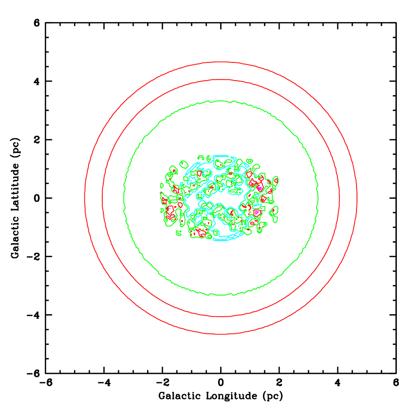
Figure 4: Density contours showing the density averaged along the line of sight of our 6 pc cubed region surrounding Sgr A* in the projected longitude/latitude plane. The contours correspond to the following average densities: magenta ($>10^{4}{\rm cm^{-3}}$), red ($10^{3}-10^{4}{\rm cm^{-3}}$), green ($10^{2}-10^{3}{\rm cm^{-3}}$), and cyan ($<10^{2}{\rm cm^{-3}}$). The torus causes an increased density in the central 2 pc region. The edge of the wind-blown bubble causes a density enhancement in a ring near 4 pc.

Clumps exist in this wind profile, the largest being the dense cores in the CND. Any model of the GC region must also include these structures. In this paper, we include only the circumnuclear disk in modeling the high-energy $\gamma$-ray emission. A number of other dense filaments (a.k.a. “streamers”) and clumps exist in this central region and we do not suggest that we are presenting a complete picture of the GC, but instead are showcasing what we can learn by using the emission from proton scattering to image the GC region. We use the circumnuclear disk as an example that the density perturbation can be imaged by this technique. The combined density structure of our wind plus bubble region and the circumnuclear torus is shown in a 2-dimensional image in Figure 4. The dense clumps in the center are the projected image of the circumnuclear disk.

3 Proton Propogation: Effective Proton Opacities

The scattering of high-energy protons with protons in our density field ultimately produces the gamma-rays that we observe in detectors such as HESS. As we shall see below, the cross-section for this scattering is quite low and this cross-section alone would produce very few gamma-rays. However, the protons can be effectively trapped by the high magnetic fields in this region and their slow diffusion out of the GC allows ample time for the protons to scatter, producing the pions that ultimately emit gamma-rays near Sgr A*. Here we discuss our model for the propogation of high-energy protons through magnetic fields, focusing on the uncertainties in this model primarily based on the uncertainties in the magnetic field topology in the GC region. We then describe the current understanding of proton-proton scattering and the simplifications we employ for our calculation of this scattering opacity.

3.1 Magnetic Field Effects

The propogation of a high-energy proton through a magnetic field can be calculated if the magnetic field strengths and distributions are well-defined. Unfortunately, especially for magnetic fields produced by turbulence and/or shocks, neither of these are true. Due to the dynamic mixing and shocks in this region, magnetic field strengths $B$ in this region are likely to be comparable to those found in typical dense clouds and, in typical star-forming regions, these magnetic fields are within an order of magnitude of their equipartition value (Padoan et al. 2004). But there is some observational evidence that the GC fields are much lower than this value (LaRosa et al. 2005). The magnetic field in our wind-blown region is shown in Fig. 5. For the most part, we assume the equipartition value for the magnetic field strength with coherent lengths below the size of our spatial resolution.

Assuming equipartition gives us a net magnetic field, but it still does not provide a distribution for the magnetic field. Can we assume that the power of the magnetic field as a function of scale-length of that field follows a Kolmogorov spectrum? Although this is commonly assumed (Blasi & Colafrancesco 1999), it is not necessarily the correct answer. We instead choose to parametrize the magnetic field energy distribution assuming a power law and vary the power to determine the dependence of our results on this uncertainty.

We use the derivation of Petrosian and Liu (2004) to parameterize the uncertainties in our magnetic field topology. With this derivation, the mean free path of particles in our magnetic field has the following form:

$$\lambda_{\rm sc}=c\gamma^{2-q}f(\beta_{\rm A})){8\over\pi(q-1)f_{\rm turb}ck_{\rm min}}\left({ck_{\rm min}\over\Omega}\right)^{2-q}~{},$$ (3)

where $c$ is the speed of light, $\beta_{\rm A}=v_{\rm A}/c$ is the Alfven velocity in the plasma in units of the speed of light, $\gamma$ and $\Omega$ are the Lorentz factor and the non-relativistic gyrofrequency of the particle, respectively. For our values of the Alfven velocity, the function $f(\beta_{\rm A})$ is only weakly dependent upon $\beta_{\rm A}$ (it scales roughly proportional to the log of $\beta_{\rm A}$ and, for the purposes of this simulation, we set it equal to a constant: $f(\beta_{\rm A})\approx 5$. $f_{\rm turb}$ is the energy ratio between the turbulence and the magnetic field (roughly 1). $k_{\rm min}$ is the minimum wave number of the magnetic field (the corresponding maximum scale length of the magnetic field is $\lambda_{\rm max}=2\pi/k_{\rm min}$) and $q$ is a power index corresponding to the distribution of this magnetic field.

This formula boils down our uncertainties in the magnetic field topology into two parameters: $k_{\rm min}$ (or $\lambda_{\rm max}$) and $q$. It implicitly assumes a power law for the magnetic field energy distribution in the range that determine the propogation of our high-energy protons. Typically, we would expect the power law to break when the gyroradius of the particle exceeds the scale length of the magnetic fields. As we increase the proton energy, the gyroradius increases, but even for a 100 TeV proton, the gyroradius is only $3.3\times 10^{14}(B/1{\rm mG})^{-1}$ cm and, based on the calculations by Rockefeller et al. (2004) of the region surrounding Sgr A*, we expect the scale-length of the magnetic field to be larger than this value: $\lambda_{\rm max}\gtrsim 10^{16}~{}{\rm cm}$. So it is likely that only a single power is needed for our simplified calculations.

For this paper, we will study two values of $q$: 1.5 and 2. If we assume $q=2$, the scattering length ($\lambda_{\rm sc}$) is independent of the energy of the proton ($\gamma$) and the magnetic field strength. With $\beta_{\rm A}<<1$ and $f_{\rm turb}\approx 1$, equation 3 becomes:

$$\lambda_{\rm sc}\approx 2\lambda_{\rm max}$$ (4)

Our only other free parameter, then, is the magnetic field scale length ($\lambda_{\rm max}$), and we test the dependence of the results on this parameter by running calculations with two values for $\lambda_{\rm max}$: $10^{15}$ and $10^{17}$ cm. If we assume $q=1.5$, we retain a mean-free path dependence both on the average magnetic field strength $B$ and the proton energy $E_{\rm prot}$:

$$\lambda_{\rm sc}\approx 2\times 10^{7}(\lambda_{\rm max}/{\rm cm})^{1/2}(B/0.1mG)^{-1/2}(E_{\rm prot}/10~{}TeV)^{1/2}{\rm cm}.$$ (5)

The bulk of our calculations use $q=1.5$. We obtain our average magnetic field strength set to the equipartition value from our wind-blown bubble calculations and a value of $\lambda_{\rm max}$ of $10^{15}~{}{\rm cm}$. In this paper, these mean free paths are modeled as effective scattering mean-free paths. The “scattering” is assumed to be isotropic and isoenergetic and serves mostly to redirect the protons, causing them to diffuse out of the Galactic Center region.

Our assumption that the magnetic field energy density is equal to the thermal density of our gas implicitly assumes that the largest scale-length of our magnetic fields is below the resolution of our models. But in much of the Galaxy, the magnetic fields are generated by the Galactic disk, not by small-scale turbulence, and the scale length of these fields can be large (parsec scales or above). In the GC region we consider for much of this paper, we focus on the magnetic-fields generated in our shocked wind bubble or in dense molecular clouds and it is likely that in this region, the scale length of the magnetic fields will be short compared to the size-scale of the hydrodynamics simulations (Rockefeller et al. 2004) that set up our initial conditions.

3.2 Proton Scattering

Magnetic fields may determine the propagation of the high-energy protons, but it is the proton-proton scattering cross-section that produces the pions that decay into the high-energy photons we observe. Suzuki et al. (2005) have fit the observed opacities for proton scattering with a relatively simple empirical function:

$$\sigma_{\rm pp}(E_{\rm prot})=S_{0}(c/v_{\rm proton})^{\kappa}E_{\rm prot}^{\delta}(1-e^{-\mu E_{\rm prot}}),$$ (6)

where

$$\delta=4.00\times 10^{-2}+5.38\times 10^{-4}\times E_{\rm prot}^{0.240},$$ (7)

$S_{0}=2.6\times 10^{-26}~{}{\rm cm^{-2}}$, $\kappa=2.23$, $\mu=1.07$ and $E_{\rm prot}$ is the proton energy in GeV and $v_{0}$ is the proton’s velocity. Most of the experimental data constraining this cross-section is below 100 GeV, but a few data points out to 2 TeV exist and this empirical formula fits this data points within the error bars. Above 2 TeV, the opacity is extremely uncertain.

Due to these uncertainties, for most of the calculations in this paper, we assume a constant value for this opacity ($3.2\times 10^{-26}~{}{\rm cm^{2}}$), leading to a mean free path for proton-proton scattering of:

$$\lambda_{\rm meanfreepath}^{\rm pion}=3.125\times 10^{25}n^{-1}_{\rm H}cm^{-2}.$$ (8)

We do include 1 calculation using the full description from equation 6, but it is a small effect compared to our other uncertainties. We will discuss the effect of such an assumption in our conclusions. Despite the fact that the proton is essentially performing a random walk away from the central black hole due to magnetic fields, most of our high energy protons do not actually scatter and decay until they hit the shocked interstellar medium region of the wind-blown bubble or the dense circumnuclear torus. For the bulk of our calculations, we will assume that the proton loses so much energy after this pion production that it is no longer able to produce further pions. Pions decay rapidly, producing high energy photons.

4 Simulating Pion Production

Since the discovery of the point source HESS J1745-290 in the GC, several models have been proposed. The $\gamma$-rays can be produced either via inverse Compton scattering by relativistic leptons (Atoyan & Dermer 2004; Quataert & Loeb 2005; Wang et al. 2006) or via hadronic processes (Aharonian & Neronov 2005; Liu et al. 2006). The recent detection of diffuse $\gamma$-ray emission in correlation with the Galactic molecular cloud density distribution suggests that there is a cosmic ray source in the GC and therefore favors the latter scenario (Aharonian et al. 2006).

Two features of this emission are worth special attention: its spectral index is identical to that of HESS J1745-290, and its brightness is more than two orders of magnitude lower than that of HESS J1745-290 (Aharonian et al. 2004, 2006). Given the large source size of the diffuse emission, its total flux is actually about a factor of 2 higher. These results set strict constraints on the possible cosmic ray sources in the Galactic Center: Sgr A*, pulsar wind nebulae, the supernova remnant Sgr A east, and stellar wind shocks (Quataert & Loeb 2005). For most of our calculations, we focus on a source arising near the black hole producing Sgr A*.

Combining the motions induced by magnetic fields with our proton-proton scattering cross-section, we have developed a Monte-Carlo technique to determine where protons of a given energy scatter. Magnetic fields act as an effective scattering opacity while proton-proton scattering acts as an absorption term (because we destroy the protons upon their first scattering). We first develop a 3-dimensional grid (typically 200 zones on a 6 pc side - 8 million zones total) and determine our two “opacities” at each grid point. We then launch packets from the center of this region (to mimic a Sgr A* or stellar wind source) and from a shell at roughly 5 pc (to mimic a Sgr A East supernova remnant source) and follow their trajectory until they scatter to produce protons. The magnetic fields are able to completely alter the direction of the proton in any zone, and we determine which adjacent zone the proton travels to by assuming a diffusion approximation. The probability the proton moves into a specific adjacent zone is inversely proportional to the magnetic field “cross-section” in that adjacent zone. In each zone, we calculate the probability for the proton to scatter and produce pions and, using a random sampler, determine whether a scattering event has occurred. We typically run 10 million particles per simulation to obtain enough statistics to make maps of the projected scattering surface.

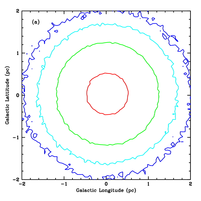
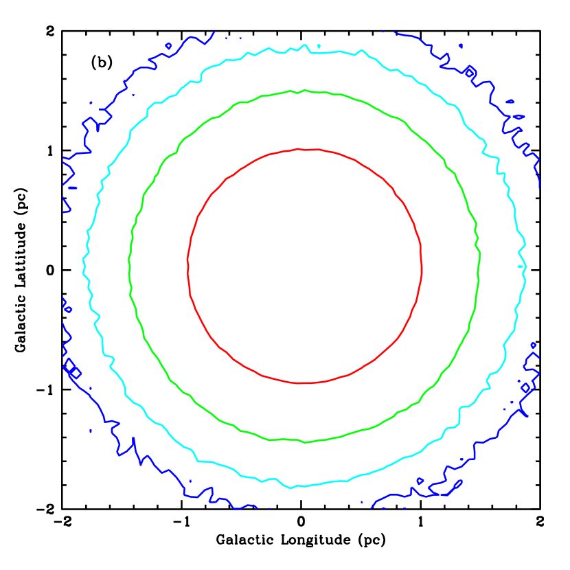
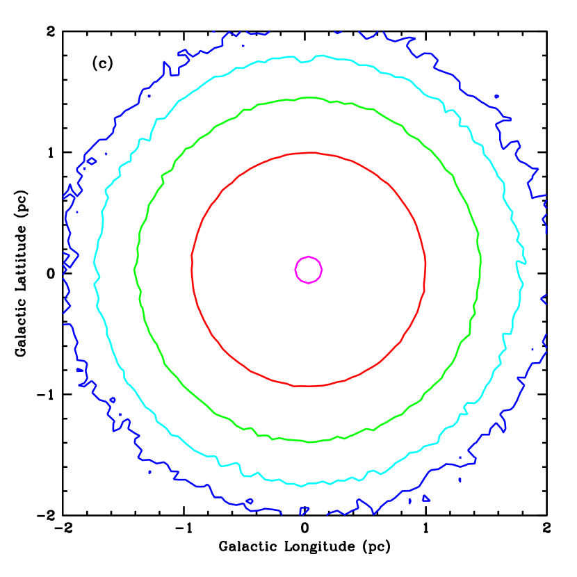
Figure 6: Contours of pion production as a function of projected surface area using our standard wind initial conditions: $\dot{M}_{\rm wind}=3\times 10^{-3}~{}{\rm M_{\odot}~{}y^{-1}}$, $v_{\rm wind}=1000{\rm kms^{-1}}$ and $\rho_{\rm MC}=10^{4}{\rm cm^{-3}}$. Each contour corresponds to the number of total pions produced in each column (we sum along the projected area to get the total “observed” production rate in each 0.06$\times$0.06 pc² zone. The contour levels correspond to fractions of: $3\times 10^{-3}$ (magneta), $3\times 10^{-4}$ (red), $3\times 10^{-5}$ (green), $3\times 10^{-6}$ (cyan), $3\times 10^{-7}$ (blue). The 3 plots correspond to (a) 1000 TeV, (b) 10 TeV, and (c) 0.1 TeV protons. Note that although the wind density is very extended, the source of pions is actually quite compact.

The photon emission is proportional to the pion production rate, and because the pion decay is rapid, the location of the $\gamma$-ray emission is at the same spot as that of the proton scattering. Hence we can use the scattering location to study the distribution of $\gamma$-rays. Before we calculate the photon energy distribution, we focus on the spatial distribution, and hence the scattering location. Our first step is to study the dependence of this spatial distribution on the proton energy. In our first series of plots, we present contours of the pion production per zone (a 0.06 pc$\times$0.06 pc square projected area) as a function of the Galactic coordinates. We normalize this production rate to the fraction of total protons launched at that energy. Figure 6 shows these contours for the wind-blown bubble density solution for 3 different proton energies: 0.1, 10, and 1000 TeV. Although the wind-blown bubble region extends beyond 2 pc, surface area effects produce the largest surface emission to be centered around the GC. As the energy of the protons increases, fewer and fewer pions are produced in the center, due to the decreased effect of magnetic fields for higher energy photons.

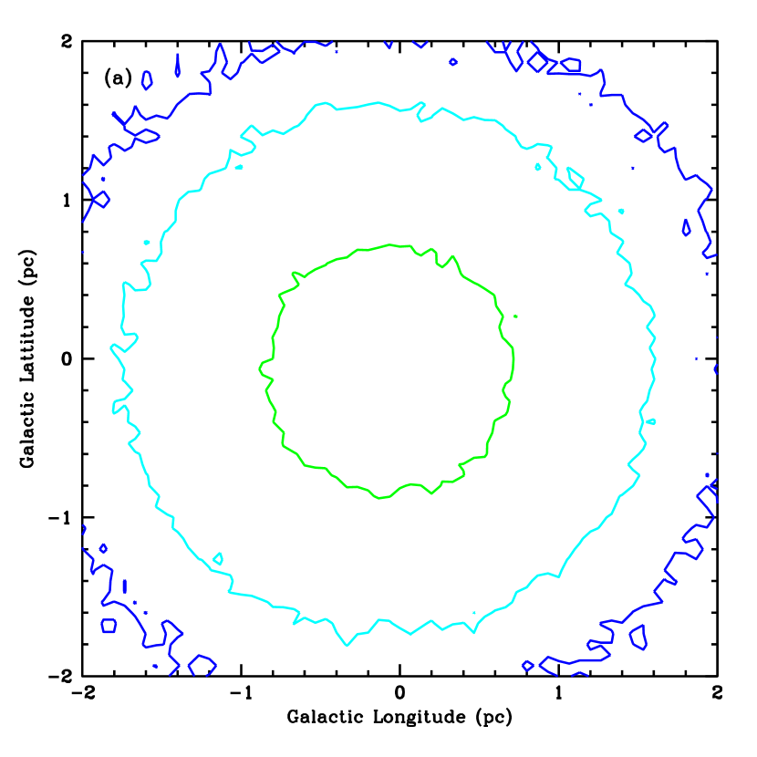
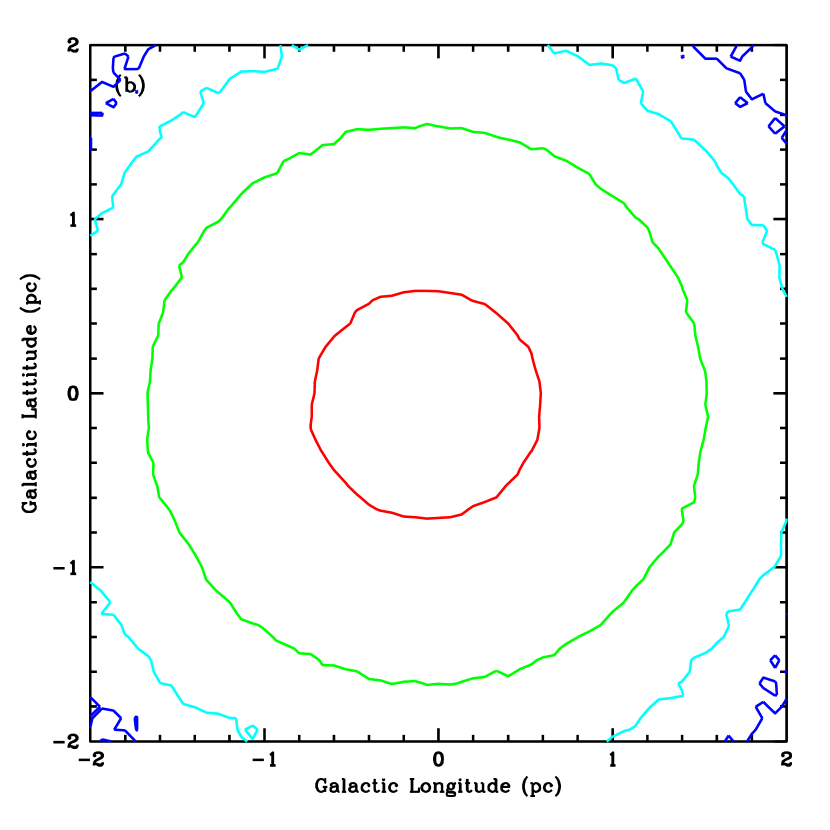
Figure 7: Same as Fig. 6 but with the density lowered by an order of magnitude and the extant of the bubble increased by $10^{0.2}$ following the calculation in equation 1.

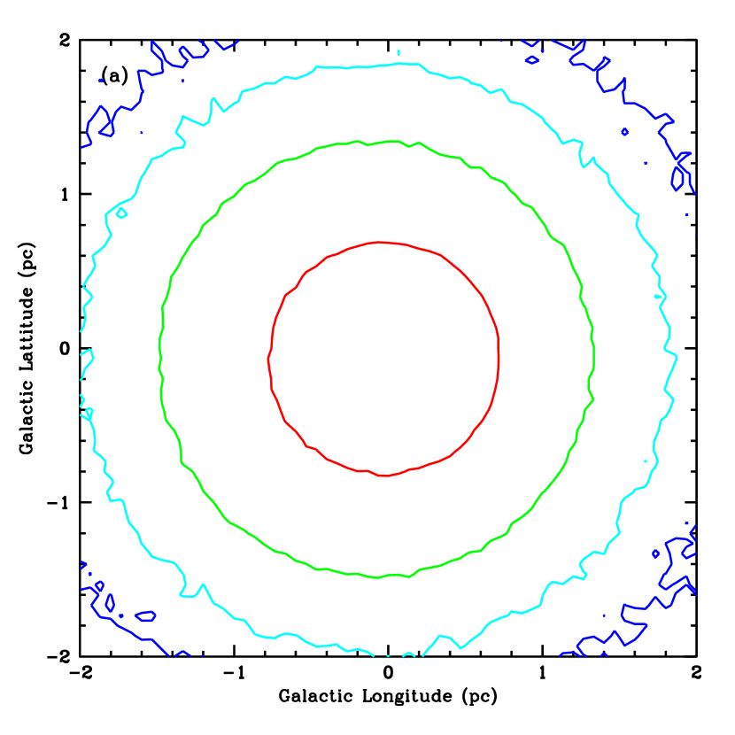
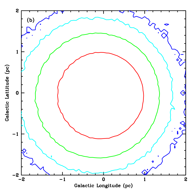
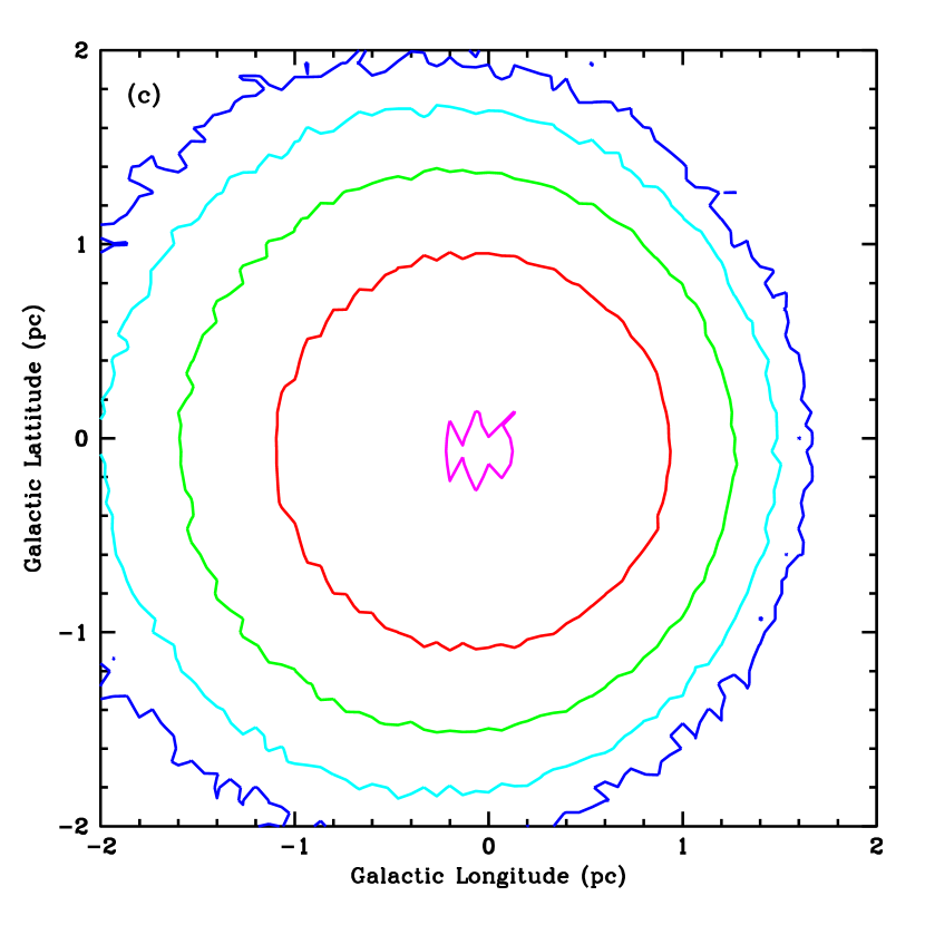
Figure 8: Same as Fig. 6 but with the density profile moved 2 pc off the center of the Galaxy.

How sensitive is this result to the details of our density profile? We also studied the effect of a lower density in the surrounding medium. Figure 7 shows the results of a simulation where this density is lowered by an order of magnitude and expanded (as we would expect from § 4). The result is fairly insensitive to this change (and will remain so until we lower the density of the molecular cloud sufficiently that the particles stream through it (below $\sim 100{\rm cm^{-3}}$). In addition, it is possible that the density profile, like Sgr A East, is offset from the center of Sgr A*, but since the winds arise from stars orbiting Sgr A*, this offset is likely to be small. As an extreme test of this uncertainty, we moved the center of the density distribution 2 pc away from Sgr A* to study the effects of such an offset. The corresponding spatial distribution of the $\gamma$-ray emission is shown in Figure 8. Although the shape is slightly changed, the result is very similar to our simple, spherically symmetric model centered on Sgr A*. Even though both of these alterations show differences from our standard model, it would be difficult, if not impossible, to observe these differences with existing telescopes.

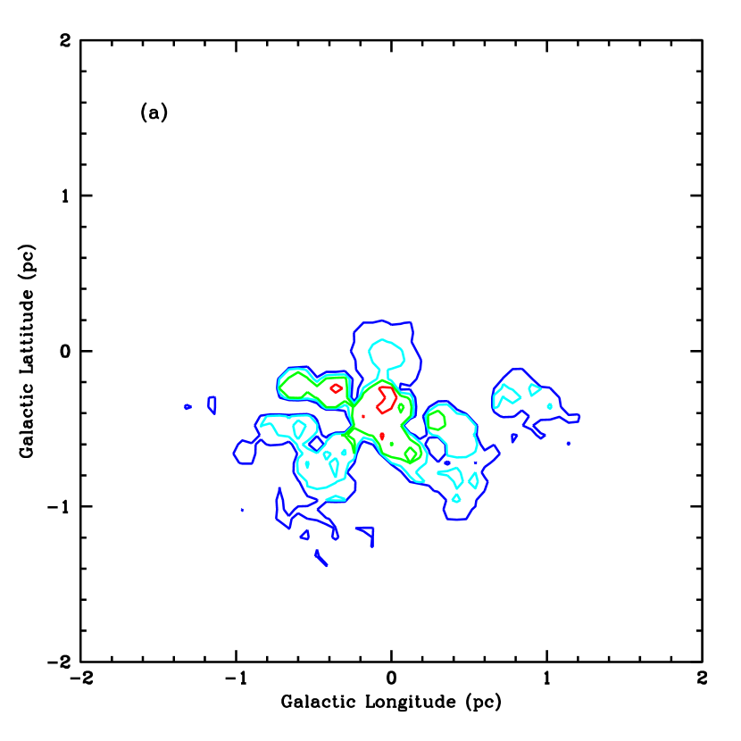
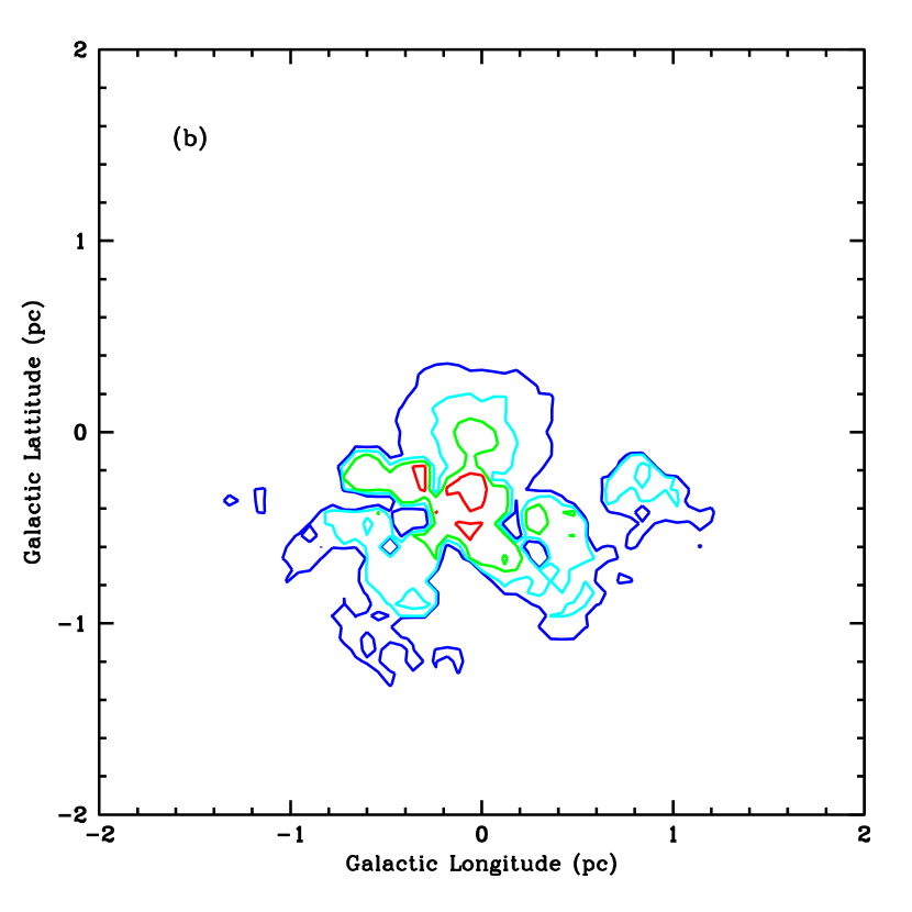
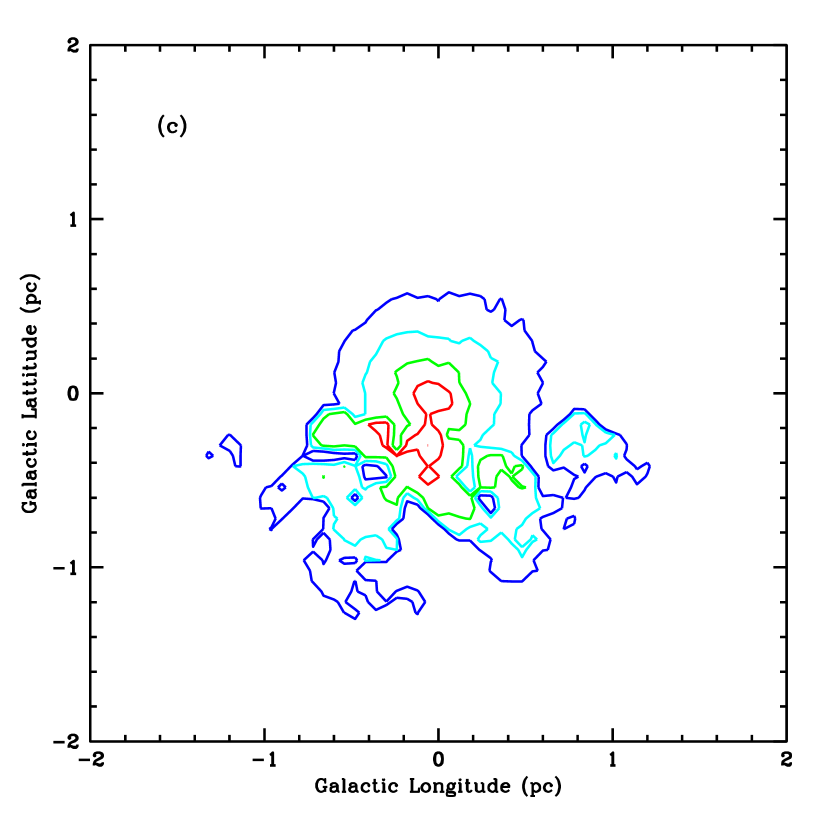
Figure 9: Same as Fig. 6 but with the density profile set by Rockefeller et al. (2004) that is dominated by the circumnuclear disk.

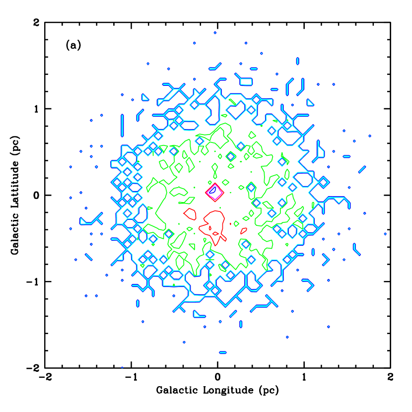
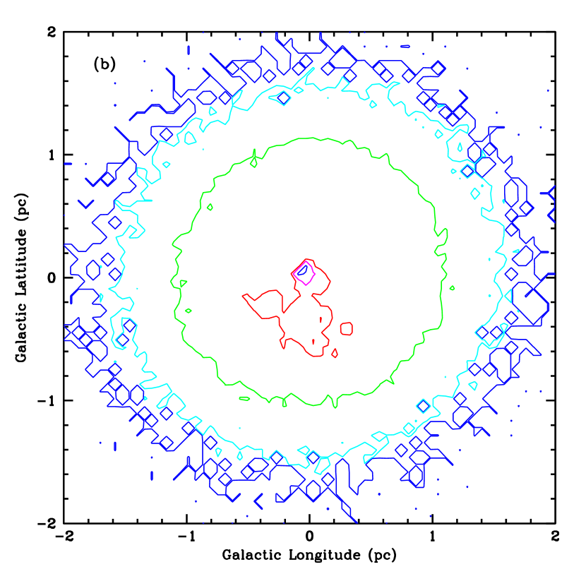
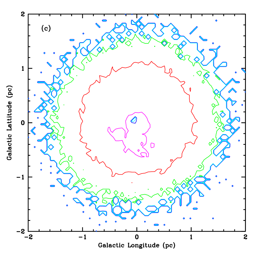
Figure 10: Same as Fig. 6, but a composite of both our wind profile and the inner density set by Rockefeller et al. (2004). This is our standard density profile for studying spectral features in § 5.

If we model the density profile produced by Rockefeller et al. (2004), the peak densities occur in the torus and right near Sgr A*. The resultant contours are far from symmetric (Fig. 9). The density structure of the circumnuclear disk is clearly shown in the image. In this manner, we can use the high energy emission to probe the density structures of the GC. This emission provides an independent means to study these densities perturbations. The combined structure, using the Rockefeller et al. (2004) density profile in the inner 2 pc and our derived wind-blown bubble structure beyond shows that dense structures such as the circumnuclear disk will still produce noticeable variations on the high-energy signature (Fig. 10).

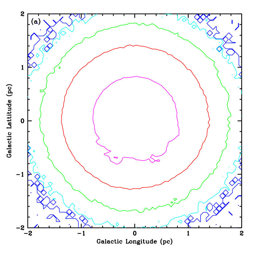
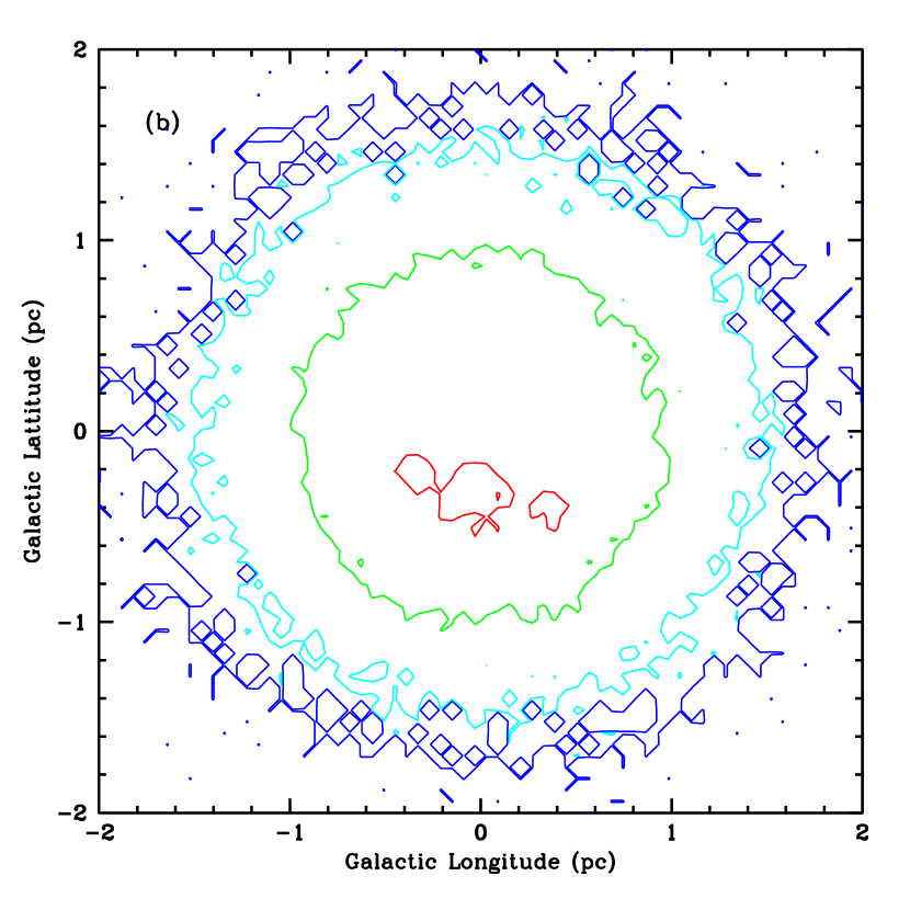
Figure 11: Same as Fig. 6, but a composite of both our wind profile and the inner density set by Rockefeller et al. (2004) using a $q$=2 value for the magnetic field distribution.

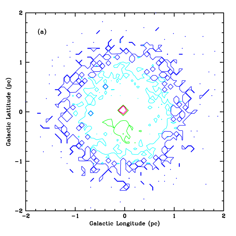
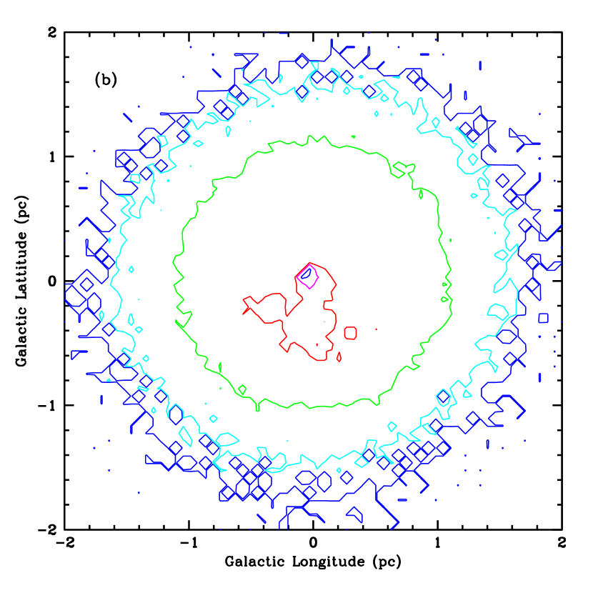
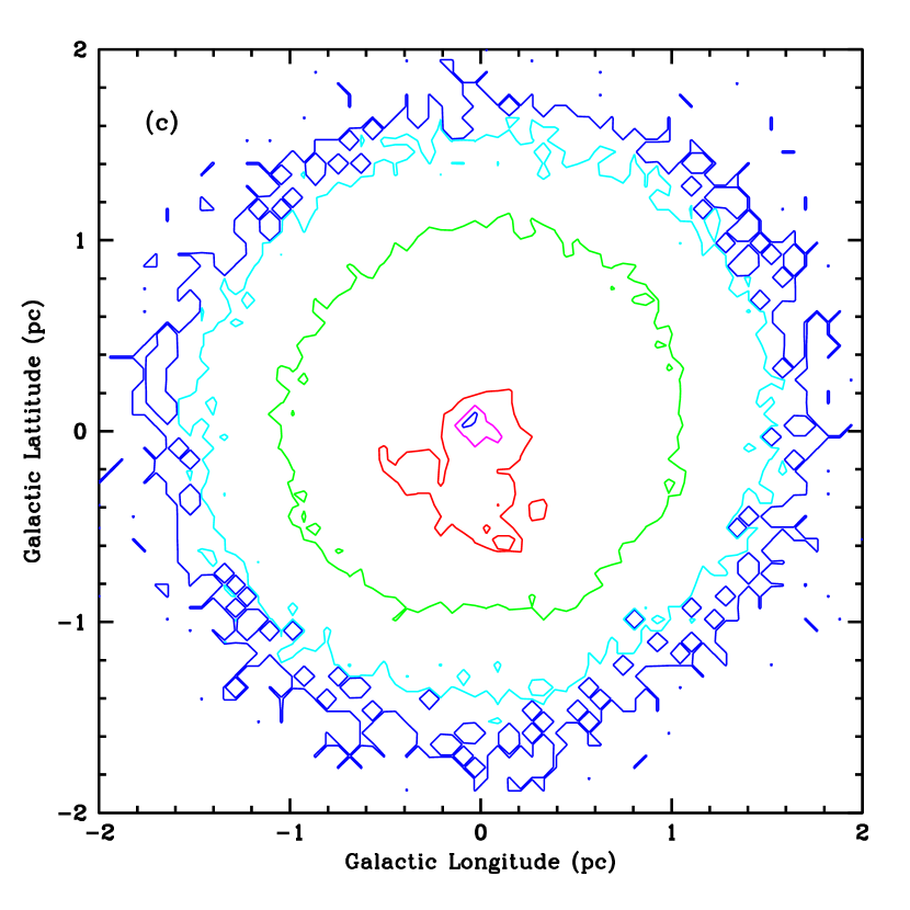
Figure 12: Same as Fig. 6, but a composite of both our wind profile and the inner density set by Rockefeller et al. (2004) using the full description of the opacity in equation 6.

How sensitive are our results to our choice of opacities? Fig. 11 shows the pion production distribution assuming that the power index for the magnetic fields is $q=2$ instead of $q=1.5$. We show plots for two scale lengths in the magnetic field: $10^{16}$ cm and $10^{18}$ cm. If the magnetic scale length is too short, much of the enhancement caused by the circumnuclear disk is washed out. Fig. 12 shows the pion production distribution with the full equation for the proton-proton scattering for 3 energies: 0.1 TeV, 10 TeV, and 1000 TeV. Over this range, the proton-proton scattering cross-section varies by less than a factor of 2 so it is not surprising that it does not change the distribution results considerably. These modifications will, however, have a larger effect on our gamma-ray spectra.

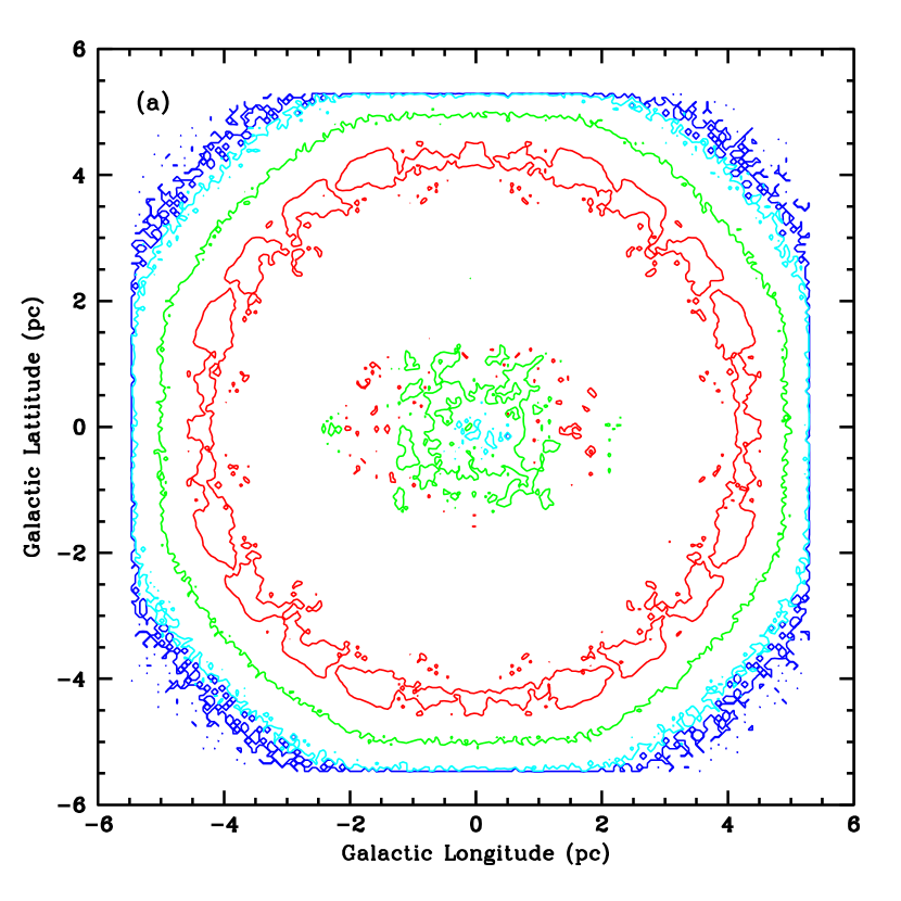
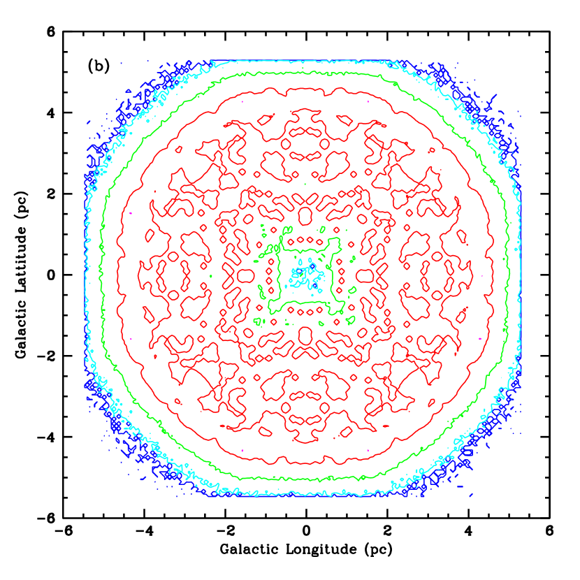
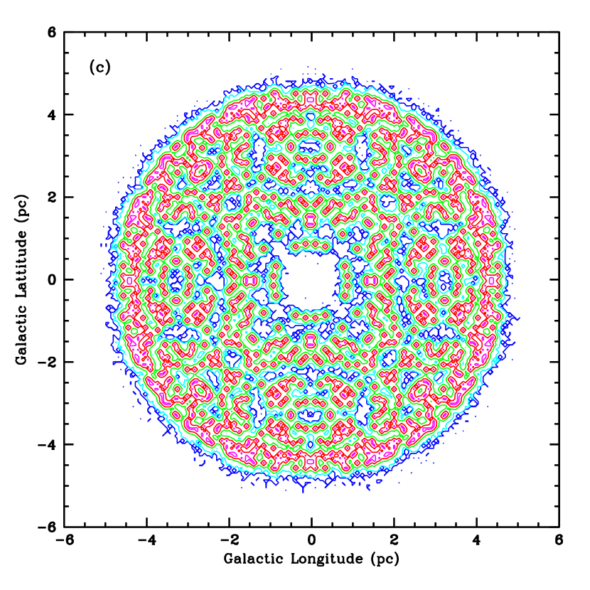
Figure 13: Same as Fig. 6, but a composite of both our wind profile and the inner density set by Rockefeller et al. (2004) using the supernova remnant Sgr A East as the source of protons. Note that this simulations produces a much more broad distribution of pion production.

Finally, can we distinguish a Sgr A East source from a more centrally located source. In all of our central source calculations, the dominant signal occurs in a projected 2 pc circle around Sgr A*. But if the source is the supernova remnant, the source will be extended (Fig. 13). Unfortunately, the distribution is still limited to a $\sim 5$ pc radial emission source in the GC, currently below the distribution resolution from HESS (Aharonian et al. 2004). If the density enhancement of Sgr A East truly is offset from Sgr A*, there is a possibility that we can distinguish this source from that of a Sgr A* source with the current data (we discuss this further below). Clearly, improved data will be able to distinguish these two sources.

A summary of our simulations is given in Table 1.

5 The High Energy Photon Emission

The plots from section 4 show the spatial distribution of the position where our protons scatter to produce pions for a set of different density profiles. Since the pions decay in less than $10^{-10}~{}$s, this is also the spatial distribution of the high-energy photons. Another way to understand the physics and the physical sources of this emission is to study the spectra produced by the different simulations. If we want to calculate the spectrum of this emission, we must estimate the energy distribution of pions and the resulting energy distribution of high energy photons.

For the energy distribution of pions, we assume a differential cross-section [$d\sigma(E_{p},E_{\pi^{0}})/dE_{\pi^{0}}$] for the proton scattering (Blasi & Colafrancesco 1999, Fatuzzo & Melia 2004):

$$d\sigma(E_{p},E_{\pi^{0}})/dE_{\pi^{0}}=\sigma_{0}f(E_{\pi^{0}}/E_{p})/E_{\pi^{0}},$$ (9)

where $E_{p}$ and $E_{\pi^{0}}$ are the proton and pion energies, respectively, $\sigma_{0}$ is the cross-section for proton scattering we used in in section 4, and $f_{\pi^{0}}(E_{\pi^{0}}/E_{p})$ is

$$f(E_{\pi^{0}}/E_{p})=0.67(1-E_{\pi^{0}}/E_{p})^{3.5}+0.5e^{-18E_{\pi^{0}}/E_{p}}.$$ (10)

If we assume momentum and energy conservation and that two photons dominate the decay, the energy distribution of the $\gamma$-ray photons we observe is flat between the limits of $(E_{\pi^{0}}-P_{\pi^{0}})/2$ and $(E_{\pi^{0}}+P_{\pi^{0}})/2$ where $P_{\pi^{0}}$ is the pion momentum. Combining these two distributions, we derive a spectrum for the $\gamma$-rays emerging from proton scattering. Note that the nature of equation LABEL:eq:dist means that the gamma-ray spectrum need not be identical to the spectrum of emitted protons, but, as we shall see, these two spectra are fairly similar.

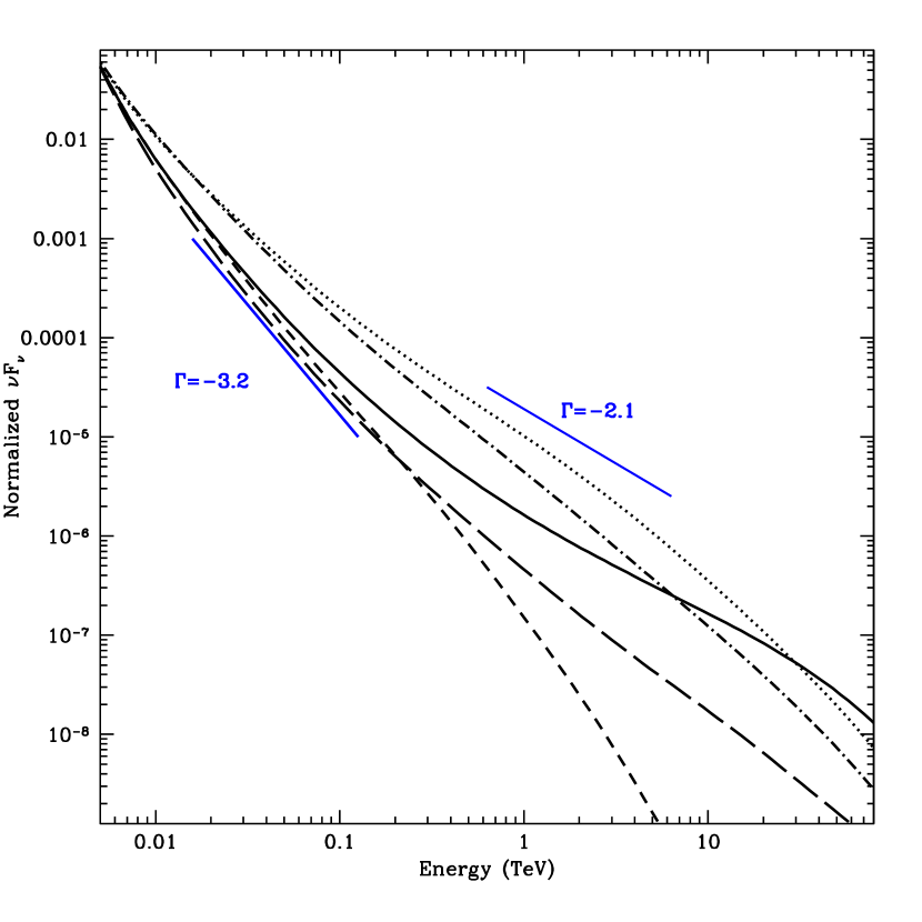
Figure 14: Normalized high-energy $\nu F_{\nu}$ fluxes per unit area as a function of energy (see Fig. 11) for 5 different models: our standard model from Fig. 11 (solid), a model only with the wind-blown bubble component (dotted), and a model with the same density profile, but with an index for the injection proton energy distribution of -3.3 (dashed), the model using the supernova remnant as a source (dot-dashed), and the model assuming $q=2$ for the magnetic field distribution (long-dashed). Clearly, if the proton energy distribution does not have a power index near -2.0, we can not get the correct slope for the gamma-rays.

To obtain an observed spectrum of $\gamma$-rays, we must first assume an injected spectrum of protons. For our standard model, we assume that the proton energy distributions falls off as $E_{p}^{-2.3}$. We include the emission protons from 10 GeV up to 1000 TeV. The exact value for this power index is fairly uncertain (we discuss the dependence on this index below). Our standard model also consists of our wind-blown bubble condition (assuming a $10^{4}{\rm cm^{-3}}$ surrounding density) with the circumnuclear disk added in the central 2 pc. The total spectrum within 6 pc is shown in Fig.14. To explain the flux of $\gamma$-rays observed by HESS from 165 GeV to 10 TeV, we need a total energy in high-energy $\gamma$-rays of $\sim 1.4\times 10^{35}~{}{\rm ergs^{-1}}$. For our simulation, such a flux would require a proton flux above 200 GeV of nearly $5\times 10^{37}~{}{\rm ergs^{-1}}$. Such values are easily within the possible proton fluxes predicted by models accelerating protons near the Sgr A* black hole (Liu et al. 2006).

Although between 10 and 100 GeV, the spectral index is close to that observed by HESS ($\Gamma\sim-2.2$), in the actual HESS regime (above 0.1 TeV), the spectral index is generally a bit steeper (below -2.2). This index depends sensitively on our assumptions of the proton energy distribution, the density profile, and the opacities. In Fermi shock acceleration models, we are restricted to source energy distributions of the protons with an index near 2. Not so with the stochastic model of Liu et al. (2006). If we assume the proton energy distribution falls off as $E_{p}^{-3.3}$, we obtain the dashed curve in Fig. 14. Here the spectral index of the $\gamma$-rays is much steeper than the observed rate. Whereas shock acceleration models predict roughly the correct energy distribution, the stochastic acceleration model must come up with an argument for getting an answer similar to the shock accleration models. For this simulation, we require a proton emission energy above 0.2 TeV of $10^{37}~{}{\rm ergs^{-1}}$ to match the HESS flux. The spectral index is also sensitive to the density distribution. Using the wind-blown bubble profile alone (with the proton distribution of $E_{p}^{-2.3}$), we obtain the dotted curve in Fig. 14. The spectral index for this simulation (using a proton spectral index of -2.3) is steeper than our corresponding combined simulation (solid curve, Fig. 14), but still within an acceptable range to fit the data. For this model, the proton flux required above 0.2 TeV would be below $10^{37}~{}{\rm ergs^{-1}}$. Similarly, we have modeled both a supernova remnant spectrum (dot-dashed) and altered opacity calculation (long-dashed). All fit the observations comparably well.

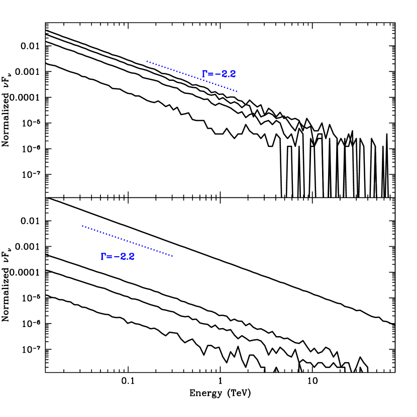
Figure 15: Normalized proton $\nu F_{\nu}$ fluxes per unit area as a function of energy for a range of separations from the GC ranging from 0.24 pc to 2.4 pc for our standard model (bottom) and the model assuming $q=2$ for the magnetic field distribution (top). Although the index does not change, as we move out, the signal gets increasingly noisy as the proton scattering rate decreases.

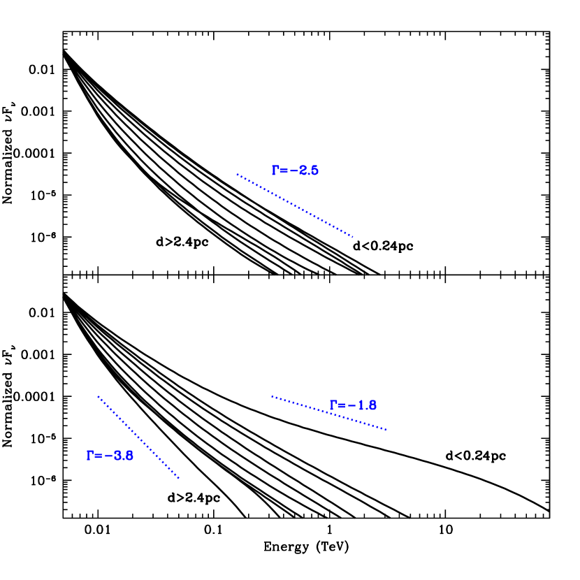
Figure 16: Normalized high-energy $\nu F_{\nu}$ fluxes per unit area as a function of energy for a range of separations from the GC ranging from 0.24 pc to 2.4 pc for our standard model (bottom) and the model assuming $q=2$ for the magnetic field distribution (top). Very close to the Galactic Center, high energy protons are absorbed, causing a flattening of the spectrum (this is especially evident in the standard model). As we move outward, the density and magnetic field drops sufficiently that essentially no high-energy protons are absorbed and the slope of the energy steepens. However, since we can only observe the total spectrum at this point, we can not constrain our opacities with the current observations.

If we had spatial information of the spectrum, we would have another set of constraints on our model. Figure 15 shows the energy distribution of our protons as a function of the position at which they scatter from 0.24 pc to 2.4 pc for our standard model (bottom) and our $q=2$ magnetic field distribution model (top). The slope does not change much, but the data gets much noiser as we move out from the center and get fewer scattering events (especially at the high energy range). The decrease in high-energy scatters will alter the slope of the gamma-ray emission. Figure 16 shows the spectrum of the $\gamma$-rays as we move out from 0.24 pc to 2.4 pc for these same two simulations. The spectral index in the 0.1-10 TeV range is approximately -1.8 close to the black hole, but falls to -3.8 if we look at material beyond 2.4 pc for our standard model. This is because so few high-energy protons scatter beyond the inner 0.5 pc of Sgr A*. Of course, this result depends sensitively on both our proton spectral index, our density distribution, and even on our choice for the power law index for the scale of our magnetic fields.

What can we take away from these calculations? Within the uncertainties in our proton emission, proton scattering, density profile, etc., we can easily match the observations of both $\gamma$-ray spectra and flux. This is simply because we have several large uncertainties that can be tuned to fit the results, and only 2 pieces of data. But, if we had more detailed information, such as the evolution of the spectral index with time, we could place stronger constraints on our models. If we had, in addition, a detailed spatial map of the emission, we could further constrain our models and ultimately get a better understanding of the magnetic field distribution and the energy distribution of our cosmic ray protons produced by our acceleration mechanism.

6 Conclusions and Future Prospects

A wind-blown bubble density structure provides an ideal first-order approximation of the $\sim 5$ pc region surrounding Sgr A*. This structure is not only a prediction of theory, but it also is supported by several observations. It allows a more reasonable estimate of the supernova explosion energy and explains the X-ray ridge observed near Sgr A*. With a single parameter (the density of the medium beyond the bubble), we can predict the size of the bubble. Bear in mind, however, that this model is still only a first-order approximation; many additional molecular structures complicate this region.

We apply this simple density structure to a specific model for the source of high-energy $\gamma$-rays near the GC: scattering of high-energy protons. Given the uncertainties in the source (both its energy and its spatial distribution), the opacities (especially the effects of magnetic fields), and the densities in the GC region, it is not surprising that we can construct multiple solutions that match the current observations. But our calculation does allow us to determine which uncertainties must be better understood to constrain the models further with the existing data. In addition, we can determine which future observations will most help us constrain the models.

We have shown that detailed spatial maps can help us study the density structure in the GC region, but if the source of protons is indeed Sgr A*, the resolution required is far beyond what we can do with current telescopes. What the observations can constrain is the source itself. If Sgr A East were the source, the emission would be quite extended. Figure 17 shows the normalized flux as a function of radius. For a source near Sgr A*, the gamma-ray emission really is point-like, within the inner 2 pc. But a Sgr A East supernova remnant source argues for an extended source of gamma-ray emission (out to 5 pc) that increases out to 5 pc and then drops precipitously. The innermost two pixels in the current data correspond roughly to 7 pc and our emission profile from Sgr A East is just barely consistent with these two pixels. The strong drop in emission at 5 pc would mean that a pixel centered at 7 pc should be a factor of 2 lower than the peak. As data improves, this emission source might be easily ruled out. But remember that Sgr A East is not a 5 pc spherical shell. If the emission is dominated by the shorter axis of Sgr A East, this emission would center around 3 pc instead of 5 pc.

The centroid of the emission also places constraints on a Sgr A East source. Sgr A East is offset by 2 pc from Sgr A*. If the centroid truly is exactly on Sgr A *, and the density profile of Sgr A East truly is offset (not just the emission), we can also rule out Sgr A East. Note that for a Sgr A* source, even if the termination shock of the wind-blown bubble is offset by 2 pc, we found that the centroid of the high energy emission does not move by more than 0.1 pc.

Finally the question arises whether the extended gamma-ray emission can be used as a constraint on the source. If we want to claim that the extended emission is produced by the same proton source as the point-like source, we can use the observations to constrain the proton source. For the Sgr A East source, the primary constraint arises because, given the new estimate for the age of the remnant by Rockefeller et al. (2006), Sgr A East has been producing high-energy protons for at most 1000 y. For those protons to emit gamma-rays 100 pc away, there must be a “hole” where the density is low and the scale-length of the magnetic field is high. The proton travel time is this distance (100 pc) times the effective optical depth of the protons divided by the speed of light. To make this timescale fall below 1000 y, this roughly requires an optical depth of less than 2-3, implying that the scale-lenght of the magnetic field is greater $\sim$ 50 pc. This timescale constraint is not important for a continuous source like Sgr A*. However, the fact that the spectral index is nearly identical suggests that either the opacities—in particular, the magnetic field effective opacity—must be energy independent or that a similar hole exists.

We can not absolutely rule out a Sgr A East source for the high energy emission, but taking all of the above constraints together, we have to introduce a number of caveats to make a Sgr A East source match the existing data. With accurate density maps and a precise localization of the high-energy source, it is likely that this source can be ruled out in a more absolute sense.

Finally, the spectral distribution of the gamma-ray emission depends on all of our uncertainties: source, opacities, and density distribution in the Galactic center. However, the spectral distribution as a function of space is an ideal probe of our opacities, in particular the distribution of the magnetic fields (compare the plots in Figure 16).

Acknowledgments This work was carried out under the auspices of the National Nuclear Security Administration of the U.S. Department of Energy at Los Alamos National Laboratory under Contract No. DE-AC52-06NA25396.

Table 1: Distribution Calculations

Source	Density	Opacity	Figure
Sgr A*	Wind	Eq. 5,8	6
Sgr A*	Wind, Low Dens.	Eq. 5,8	7
Sgr A*	Wind, Offset	Eq. 5,8	8
Sgr A*	Torus	Eq. 5,8	9
Sgr A*	Torus+Wind	Eq. 5,8	10
Sgr A*	Torus+Wind	Eq. 4,8	11
Sgr A*	Torus+Wind	Eq. 5,6	12
Sgr A East	Torus+Wind	Eq. 5,6	13

Figure 1: Velocity (top) and density (bottom) versus radius of the wind-blown bubble created by our standard set of conditions: a $3\times 10^{-3}{\rm M_{\odot}~{}s^{-1}}$, $1000~{}{\rm km~{}s^{-1}}$ wind blowing into a density of $10^{4}{\rm cm^{-3}}$. This structure is 110,000 y after the onset of the wind. We have separated the structure into 4 regions: free-streaming wind material (with its density falling off as the square of the radius), shocked wind material, shocked molecular cloud material (the outer edge of this region marks the end of the wind bubble), and unshocked (“cold”) molecular cloud material.

Figure 2: Velocity (top) and density (bottom) of our standard set of wind conditions for 3 different times: 60,000 y, 110,000 y, and 230,000 y. The edges of all the regions move outward with time. For instance, the outer edge of the shocked molecular cloud region (edge of the wind-blown bubble) moves 3.7 pc in the first 60,000 y, 1.2 pc in the next 50,000 y (a total of 4.9 pc in 110,000 y), and 1.7 pc in the next 120,000 y (a total of 6.6 pc in 230,000 y). If we were modeling turbulence and cooling in the shock, when the outward motion of the shock decelerated below the turbulent velocity, the wind bubble would stall. Because our molecular cloud is cool (and because we include its self-gravity), it gradually compresses, causing a slight rise in the density at late times.

Figure 3: Radius and expansion velocity of the wind-blown bubble as a function of time for three values of $\dot{M}_{wind}v^{2}_{\rm wind}/\rho_{\rm MC}$: our standard values (solid line), a factor of 10 increase in this value (dotted line), and a factor of 10 decrease in this value (dashed line). When the velocity of expansion drops below the turbulent (or sound speed velocity), the effective expansion of the bubble halts. Note that this happens before the wind-blown bubble is 100,000 y old. We can safely assume that the bubble produced by the stars surrounding Sgr A* has reached this steady state.

Figure 5: Magnetic field in mG for the wind blown bubble assuming the magnetic field energy is in equipartition with the thermal energy of the matter. The shocked regions have high values as their temperatures, and hence energies, are high.

Figure 17: Normalized flux per radial bin as a function of radius for our standard (solid), $q=2$ for the magnetic field distribution (dashed) and Sgr A East source (dotted) simualtions. The Sgr A East gamma-ray emission is much more extended.

References

- Aharonian et al. (2002) Aharonian, F.A., Belyanin, A.A., Derishev, E.V., Kocharovsky, V.V., & Kocharovsky, Vl.V. 2002, PRD, 66, 023005
- Aharonian et al. (2004) Aharonian, F. A. et al. 2004, A&A, 425, 13
- Aharonian et al. (2005) Aharonian, F. A. and Neronov, A. 2005, ApJ, 619, 306
- Aharonian et al. (2006) Aharonian, F. A., et al. 2006, Nature, 439, 695
- Albert et al. (2006) Albert, J., et al. 2006, ApJ, 638, L101
- Atoyan & Dermer (2004) Atoyan, A., & Dermer, C. D. 2004, ApJ, 617, L123
- Blasi & Colafrancesco (1999) Blasi, P., & Colafrancesco, S. 1999, Astropart. Phys., 12, 169
- Brown, Hartmann, & Burton (1995) Brown, A.G.A., Hartmann, D., & Burton, W.B. 1995, A&A, 300, 903
- Chevalier & Li (1999) Chevalier, R.A., & Li, Z.-Y. 1999, ApJ, 520, L29
- Fatuzzo and Melia (2003) Fatuzzo, M. and Melia, F. 2003, ApJ, 596, 1035
- Fryer et al. (1999) Fryer, C.L., Benz, W., Herant, M., & Colgate, S.A. 1999, ApJ, 516, 892
- Fryer, Rockefeller & Young (2006) Fryer, C.L., Rockefeller, G., & Young, P.A. 2006, accepted by ApJ
- Fryer et al. (2006) Fryer, C.L., Rockefeller, G., Hungerford, A.L., Melia, F. 2006, ApJ, 638, 786
- Heger et al. (2003) Heger, A., Fryer, C.L., Woosley, S.E., Langer, N., & Hartmann, D.H. 2003, ApJ, 591, 288
- Herrnstein & Ho (2004) Herrnstein, R.M., & Ho, P.T.P. 2004, ANS, 1, 583
- Herrnstein & Ho (2005) Herrnstein, R.M., & Ho, P.T.P. 2005, ApJ, 620, 287
- Hinton et a. (2006) Hinton, J. for H.E.S.S. Collaboration 2006, astro-ph/0607351
- Kosack et al. (2004) Kosack, K. and Collaboration, t. V. 2004, astro-ph/0403422
- LaRosa et al. (2005) LaRosa, T.N., Brogan, C.L., Shore, S.N., Lazio, T.J., Kassim, N.E., Nord, M.E. 2005, ApJ, 626, L23
- Liu, Melia, & Petrosian (2006) Liu, S., Melia, F., and Petrosian, V. 2006, ApJ, 636, L798
- Mezger et al. (1989) Mezger, P.G., Zyka, R., Salter, C.J., Wink, J.E., Chini, R., Kreysa, E., & Tuffs, R. 1989, ApJ, 209, 337
- Nomoto et al. (2004) Nomoto, K., Maeda, K., Mazzali, P.A., Umeda, H., Deng, J., & Iwamoto, K., in “Stellar Collapse”, Astroph. & Space Science Library, ed. Chris Fryer, Kluwer Academic Publishers (Dordrecht)
- Padoan et al. (2004) Padoan, P., Jimenez, R., Juvela, M., & Nordlund, A. 2004, ApJ, 604, L49
- Petrosian & Liu (2004) Petrosian, V., & Liu, S. 2004, ApJ, 610, 550
- Post (1956) Post, R. F. 1956, Rev. Mod. Phys., 28, 338
- Priddey et al. (2006) Priddey, R.S., Tanvir, N.R., Levan, A.J., Fruchter, A.S., Kouveliotou, C., Smith, I.A., & Wijers, R.A.M.J. 2006, MNRAS, 369, 1189
- Quataert & Loeb (2005) Quataert, E., & Loeb, A. 2005, ApJ, 635, 45
- Rockefeller, Fryer, Melia, & Warren (2004) Rockefeller, G., Fryer, C. L., Melia, F., and Warren, M. S. 2004, ApJ, 604, 662
- Rockefeller et al. (2005) Rockefeller, G., Fryer, C.L., Baganoff, F.K., & Melia, F.
- Tsuchiya et al. (2004) Tsuchiya, K. et al. 2004, ApJ, 606, L115
- Wang et al. (2006) Wang, Q. D., Lu, F. J., & Gotthelf, E. V. 2006, MNRAS, 367, 937
- Yan & Lazarian (2002) Yan, H., & Lazarian, A. 2002, Phys. Rev. Lett., 89, 281102