Temperature profiles of a representative sample of nearby X-ray galaxy clusters

Abstract

Context. A study of the structural and scaling properties of the temperature distribution of the hot, X-ray emitting intra-cluster medium of galaxy clusters, and its dependence on dynamical state, can give insights into the physical processes governing the formation and evolution of structure.

Aims. Accurate temperature measurements are a pre-requisite for a precise knowledge of the thermodynamic properties of the intra-cluster medium.

Methods. We analyse the X-ray temperature profiles from XMM-Newton observations of 15 nearby ($z<0.2$) clusters, drawn from a statistically representative sample. The clusters cover a temperature range from 2.5 keV to 8.5 keV, and present a variety of X-ray morphologies. We derive accurate projected temperature profiles to $\sim 0.5\,R_{200}$, and compare structural properties (outer slope, presence of cooling core) with a quantitative measure of the X-ray morphology as expressed by power ratios. We also compare the results to recent cosmological numerical simulations.

Results. Once the temperature profiles are scaled by an average cluster temperature (excluding the central region) and the estimated virial radius, the profiles generally decline in the region $0.1\,R_{200}\lesssim R\lesssim 0.5\,R_{200}$. The central regions show the largest scatter, attributable mostly to the presence of cool core clusters. There is good agreement with numerical simulations outside the core regions. We find no obvious correlations between power ratio and outer profile slope. There may however be a weak trend with the existence of a cool core, in the sense that clusters with a central temperature decrement appear to be slightly more regular.

Conclusions. The present results lend further evidence to indicate that clusters are a regular population, at least outside the core region.

1 Introduction

The temperature and density are the key measurable characteristics of the hot, X-ray emitting intracluster medium (ICM). The determination of important derived properties such as entropy, pressure, and, under the assumption of hydrostatic equilibrium, the total mass, is dependent on accurate estimation of these quantities. Because of limited photon statistics it is usual to measure the density and temperature in terms of radial profiles. However, while the density of the ICM is relatively easy to measure from the surface brightness profile of a given cluster, the temperature determination requires sufficient photon statistics to build, and fit, a spectrum. Thus ICM temperature profiles are typically determined with considerably less spatial resolution than density profiles.

The measurement of radial temperature profiles is further complicated by the density squared ($n_{e}^{2}$) dependence of the X-ray emission. The steep drop of the X-ray surface brightness with distance from the centre, combined with the background from cosmic, solar and instrumental sources, makes accurate measurement of the temperature distribution at large distances from the centre a technically challenging task.

The earliest temperature profiles were measured with Einstein, EXOSAT, Spacelab-2 and GINGA only for the nearest, brightest clusters (e.g., Fabricant, Lecar & Gorenstein 1980; Fabricant & Gorenstein 1983; Hughes, Gorenstein & Fabricant 1988; Eyles et al. 1991; Koyama, Takano & Tawara 1991). The low, stable background of ROSAT made possible spatially resolved spectroscopy of poor clusters (e.g. David, Jones & Forman, 1995); however, limited spectral resolution and bandwidth made such measurements difficult for hotter clusters (e.g. Henry, Briel & Nulsen, 1993; Briel & Henry, 1994; Henry & Briel, 1995). ASCA and BeppoSAX had sufficient high-energy sensitivity to accurately measure the temperatures of hot clusters. However both of these satellites suffered from significant PSF blurring, which, in the case of ASCA, was exacerbated by a significant energy dependence. As a result, at the end of the ASCA/BeppoSAX era, the exact shape of cluster temperature profiles was still under vigorous debate (Markevitch et al., 1998; Irwin, Bregman & Evrard, 1999; White, 2000; Irwin & Bregman, 2000; Finoguenov et al., 2001; De Grandi & Molendi, 2002).

Chandra and XMM-Newton do not suffer from major PSF problems. The on-axis Chandra PSF is negligible, while the XMM-Newton PSF becomes an issue only for clusters with very centrally peaked core emission; in addition, neither is energy-dependent. Recent observations of moderately large samples consisting primarily of nearby cooling core clusters with XMM-Newton (Piffaretti et al., 2005) and Chandra (Vikhlinin et al., 2005) have largely validated the original ASCA results of Markevitch et al., which suggested that temperature profiles declined from the centre to the outer regions. However, other Chandra and XMM-Newton observations have found flatter profiles (Allen et al., 2001; Kaastra et al., 2004; Arnaud et al., 2005). As of the time of writing, no systematic attempt has been made, with either XMM-Newton or Chandra, to look at the temperature profiles of a representative sample of nearby clusters. Although other projects on representative samples are in progress (e.g., Reiprich et al., 2006), they are not expected to be able to map the temperature distribution out to large radius.

In this paper we deal with observations of 15 clusters from a statistically representative sample observed with XMM-Newton . We describe in detail the data reduction and background subtraction, and compare our results with previous work and with those from cosmological hydrodynamical simulations. We also make a preliminary investigation of correlations with quantitative morphological measures. We present only projected temperature profiles in this paper – such profiles are direct observables and do not depend on complicated PSF and deprojection algorithms. We will deal with correction of the profiles in forthcoming papers which make use of observations of the full sample. All results are given assuming a $\Lambda$CDM cosmology with $\Omega_{m}=0.3$ and $\Omega_{\Lambda}=0.7$ and $H_{0}=70$ km s^-1 Mpc^-1. Unless otherwise stated, errors are given at the $68$ per cent confidence level.

2 The sample

The XMM-Newton Legacy Project for the study of cluster structure was initiated to study the structural and scaling properties of a large, representative sample of clusters. Since full details will appear in a forthcoming paper, we present here only a short summary of the sample selection.

The parent sample is the REFLEX catalogue (Böhringer et al., 2004). To ensure the best quality for potential targets, the REFLEX catalogue was first screened to include only objects which had (i) a firm detection threshold of more than 30 source photons in the ROSAT All Sky Survey and (ii) a low column density ($n_{H}<6\times 10^{20}$ cm^-2).

Since the Legacy Project selection was intended to be representative of an X-ray flux- or $L_{X}$-limited sample, clusters were chosen purely on the basis of X-ray luminosity. Further selection criteria included: (i) redshift $z<0.2$ to sample the nearby Universe; (ii) close to homogeneous coverage of the luminosity space; (iii) a flux limit corresponding to ${\rm k}T>2$ keV, to sample the mass range from poor systems to rich clusters; (iv) detectable with XMM-Newton to approximately a radius of $R_{500}$, with distances selected to optimise $R_{500}$ in the XMM-Newton field of view.

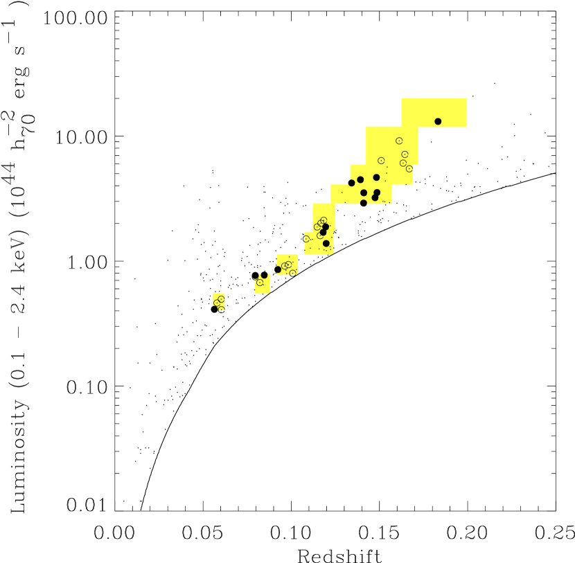
Figure 1: X-ray luminosity - redshift ( $L_{X}-z$) distribution of the REFLEX cluster sample in the redshift range $0<z<0.25$. The redshift/luminosity selection for the Legacy Project sample is indicated by the boxes. Filled circles indicate clusters from the Legacy Project which are discussed in this paper; dotted circles indicate clusters for which re-observations are necessary. The solid line is the REFLEX flux limit. (This figure is available in colour in the online version of the journal.)

To best assess the scaling relations, the sample should have close to homogeneous coverage of luminosity space. The luminosity-redshift space was thus sampled in eight almost-equal luminosity bins (see Fig. 1). The lower redshift boundary of each bin was placed above the flux limit curve or close to the curve defining the redshift at which $R_{500}$ corresponds to $9\arcmin$ ($10\arcmin$ for the most luminous clusters). The upper redshift boundaries were defined by the number of clusters to be included in the bin (4 objects). For the lowest luminosity bin these criteria were relaxed, and the bin put at lower redshift, because these clusters are fainter. The distribution of clusters in luminosity-redshift space is shown together with the luminosity bins chosen for the Legacy Project sample in Fig. 1.

Observations of the full sample of 31 clusters plus 2 archive observations have now been completed. As detailed below, the quality of 18 of these observations is not sufficient to derive accurate radial temperature profiles to relatively large radius. The remaining 15 clusters with good quality data are discussed in this paper. As shown in Fig. 1, only one redshift bin is not represented in this subsample, thus it is representative of the sample as a whole.

3 XMM data analysis

Observation data files (ODFs) were retrieved from the XMM archive and reprocessed with the XMM-Newton Science Analysis System (SAS) v6.1 using the publicly-available calibration current as of February 2005. The resulting calibrated EMOS and EPN event files were then used in all subsequent analysis.

3.1 ODF preparation

The data were cleaned for periods of high background due to soft proton solar flares using a two stage filtering process. A light curve was first extracted in 100 second bins in the [10-12]/[12-14] (EMOS/EPN) energy band. A Poisson distribution was fitted to a histogram of this light curve, and $\pm 3\sigma$ thresholds calculated. A Good Time Interval (GTI) file was produced using the upper threshold, and the event list was filtered accordingly. Since i) flares often appear to have soft ‘wings’; ii) the statistics at high energy are often poor; and iii) softer flares exist, the event list was then re-filtered in a second pass. In this case light curves were made in 10 sec bins in the full [0.3-10] band, the smaller bin size being possible because of the greatly improved statistics. A histogram was calculated, a Poisson distribution fitted, GTIs generated, and event lists were filtered as above.

Table 1: Basic cluster data.

RXCJ	$T_{X}$	z	$N_{H}$	Exp.	Comments
0003+0203	$3.71\pm 0.09$	0.085	4.7	26,26,17	A2700
0020-2542	$5.74\pm 0.13$	0.141	2.2	16,16,11	A22
0547-3152	$6.59\pm 0.12$	0.148	2.1	23,24,17	A3364
0605-3518	$4.68\pm 0.11$	0.139	4.5	22,23,14	A3378
1044-0704	$3.56\pm 0.05$	0.134	3.6	26,26,18	A1084
1141-1216	$3.60\pm 0.08$	0.120	3.2	28,28,22	A1348
1302-0230	$3.60\pm 0.08$	0.085	1.7	25,25,16	A1663
1311-0120	$8.45\pm 0.12$	0.183	1.8	36,37,29	A1689
1516+0005	$4.34\pm 0.07$	0.120	5.4	26,27,21	A2050
1516-0056	$3.75\pm 0.10$	0.120	5.4	29,30,22	A2051
2023-2056	$2.83\pm 0.08$	0.056	5.4	17,18,10	S868
2048-1750	$3.96\pm 0.08$	0.148	4.7	25,25,19	A2328
2129-5048	$3.84\pm 0.10$	0.080	2.2	21,22,11	A3771
2217-3543	$4.60\pm 0.08$	0.148	6.6	24,24,17	A3854
2218-3853	$5.84\pm 0.17$	0.141	5.7	21,22,11	A3856

This type of flare filtering is sufficient in the majority of cases. However, it is not as effective in removing flares in cases of data sets with softly-varying count rates or gradually increasing or decreasing count rates. The histograms of such data sets invariably have a Poisson distribution with a tail, which is not well fitted with a single component. All light curve histogram fits were thus carefully examined before further analysis. In problem cases, the data sets were cleaned by hand (generally by estimating the flare periods by eye, and excluding them).

Since the object of the present work is to obtain relatively high-quality temperature profiles, we only use those observations with a cleaned EPN exposure time greater than 10 ks. Of the 33 clusters in the Legacy Project sample, 15 meet this criterion at the present time.. These observations are listed in Table 1. Figure 1 shows the X-ray luminosity - redshift distribution of the LP clusters. Filled circles show the clusters discussed in this paper, while open circles show clusters for which data are pending. REFLEX clusters appearing in the boxes include those for which the X-ray criteria (minimum 30 source photons and column density $n_{H}<6\times 10^{20}$ cm^-2) were not met. The current subsample is clearly representative of the whole sample; only one redshift bin is not represented.

After removal of periods of high soft proton flux, events were filtered according to PATTERN and FLAG criteria. For EMOS event files singles, doubles, triples and quadruples were selected (PATTERN < 13), while for EPN data sets singles and doubles were selected (PATTERN < 5). Events not corresponding to these criteria were removed from the event files before further processing. In addition, for all cameras events next to CCD edges and next to bad pixels were excluded ( FLAG==0).

To correct for vignetting, a WEIGHT column was added to each event list using the SAS task evigweight. All subsequent science products were extracted from this column as described in Arnaud et al. (2001).

Serendipitous and point sources were detected in a broad band ([0.3-10.0] keV) coadded EPIC image using the SAS wavelet detection task ewavdetect, with a detection threshold set at $5\sigma$. Detected sources were excluded from the event file for all subsequent analysis.

3.2 Background preparation

3.2.1 Flare cleaning

The basic background files used are those of Read & Ponman (2003), which have nominal exposure times of $\sim 1$ Ms/400 ks (EMOS/EPN). Close inspection of the high-energy band light curves showed that considerable periods of high soft proton flux still existed in the event files. These periods were removed by two applications of the double pass filtering procedure described in Sect. 3.1 above. The resulting filtered background event lists have light curve histograms which are adequately described by a standard Poisson distribution. The loss in exposure time is $\sim 200/100$ ks (EMOS/EPN); the larger relative EPN time loss reflects the greater EPN sensitivity to flares.

After flare filtering, the same PATTERN and FLAG selections as above were applied to the background event files. The background files were then corrected for vignetting via the addition of a WEIGHT column to the event lists.

3.2.2 Exposure correction

Since the background data sets consist of stacked observations with sources removed, exposure times can vary by up to a factor of two across the detector. Using the exposure maps supplied by Andy Read , a new exposure map was computed for each event list taking into account exposure variations due to the point source subtraction. These exposure maps were renormalised to the new exposure time of the background files after flare cleaning. An EXPOSURE column, containing the exposure time at the position of the event, was then added to each background file. The WEIGHT column was then corrected for exposure variations by simply dividing by the EXPOSURE column.

3.3 Background subtraction

The blank sky backgrounds are recast onto the sky using the aspect information from the cluster pointing, enabling extraction of source and background spectra from the same detector regions. This procedure is necessary because the spatial distribution of the various instrumental lines is not constant across the field of view.

3.3.1 Quiescent background

The XMM-Newton EMOS and EPN backgrounds are dominated by charged-particle events above $\sim 2$ keV. The intensity of this component can vary by typically $\pm 10\%$, and must be accounted for by renormalisation. The renormalisation factor for each observation was calculated in the source-free [10-12]/[12-14] kev (EMOS/EPN) energy band, and the WEIGHT column of each background file was adjusted accordingly. This renormalisation assumes that the particle induced background can simply be scaled depending on the count rate. The renormalisation factors are listed in Table 2.

3.3.2 Soft diffuse X-ray background

The observation and blank field event files contain a component due to the soft diffuse X-ray background, which dominates the flux below $\sim 1$ keV. This component is variable across the sky, and thus from pointing to pointing. Correction for this variation is thus needed.

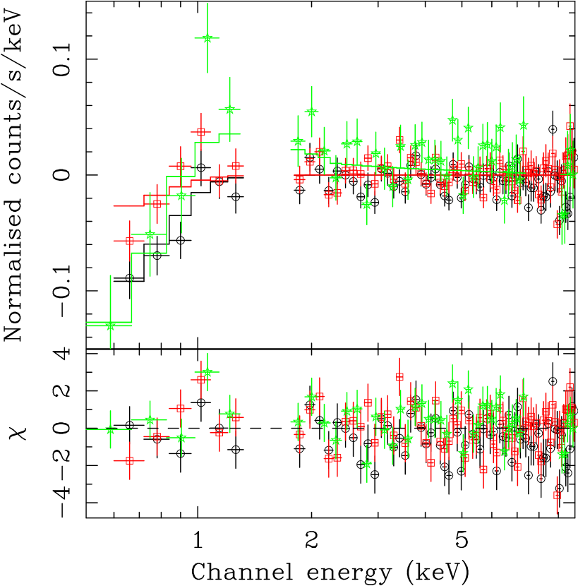
Figure 2: The residual spectrum of R0547, indicating oversubtraction of the soft X-ray background (see text for details). Black: EMOS1; red: EMOS2; green: EPN. The fit is a Solar abundance MEKAL model with ${\rm k}T=0.24$ keV and negative normalisation. The EPN model has an additional power-law component with positive normalisation. (This figure is available in colour in the online version of the journal.)

As discussed above in Sect 2, the present cluster sample was explicitly defined so that a certain fraction of the detector area is essentially free of cluster emission, enabling a direct estimation of the local background in the outer regions of the field of view. For each observation, we extracted surface brightness profiles in the [0.3-3.0] keV band for each camera. EMOS and EPN surface brightness profiles were background subtracted, coadded, and binned to $3\sigma$ significance. The local background spectrum was built using all events outside the radius at which the surface brightness profile in no longer significantly detected. A renormalised spectrum from the same region of the blank sky background was then subtracted, yielding a residual spectrum. We fitted the residual spectrum in the [0.5-10.0] keV band with an unabsorbed, solar abundance MEKAL model. Energies with significant instrumental line emission (1.4-1.6 keV for all instruments; 7.45-9. keV for EPN) were excluded from the fits. In case of a significant excess of counts in the $\gtrsim 2$ keV band, presumably due to a remaining component of soft protons, a power-law was added to the model. The EPIC spectra were fitted simultaneously, with the temperature of the MEKAL model linked between instruments. The power-law slope and normalisations of all components were free to vary in the fitting process. The normalisation of the MEKAL model was allowed to be negative, to account for over-subtraction. This purely phenomenological model is capable of describing a wide variety of residual spectra (Fig. 2), although care must be exercised in deriving the initial model parameters. This residual model, with all parameters fixed and the normalisation scaled appropriate to the ratio of extraction region areas, was treated as an additional component in all subsequent annular fits.

Table 2: Columns: (1) Cluster name; (2) Radius beyond which external region spectra were accumulated (EMOS1,EMOS2,EPN); (3-5) Normalisation factor for background rescaling. This factor was calculated from the ratio of the count rate in the observation and background files in the [10-12]/[12-14] keV (EMOS/EPN) energy band; (6) Temperature of MeKaL model used to describe the residual spectrum; (7-9) xspec normalisation of the MeKaL model used to describe the residual spectrum, in units of $10^{-4}$.

RXCJ	$R_{\rm ext}$	Normext			${\rm k}T_{\rm ext}$	MeKaL norm
	( ′ )	EMOS1	EMOS2	EPN		EMOS1	EMOS2	EPN
0003 +0203	11,11,11	1.07	0.98	1.12	0.23	-1.01	-2.98	-0.54
0020 -2542	11,11,12.5	1.00	0.98	1.02	0.10	-14.32	-20.02	-6.00
0547 -3152	11,11,11	0.99	0.93	1.04	0.24	-1.38	-0.31	-0.76
0605 -3518	11,11,11	1.22	1.18	1.19	0.26	-1.74	-1.09	-0.42
1044 -0704	10,10,10	1.14	1.11	1.16	0.26	-2.16	-0.67	-5.00
1141 -1216	11,11,11	1.06	1.04	1.13	0.27	-1.22	-1.26	-0.40
1302 -0230	11,11,11	1.04	1.02	1.07	0.27	-0.81	-0.97	-0.41
1311 -0120	11,11,11	0.97	0.93	1.05	0.19	0.95	0.95	0.95
1516 +0005	12.5,12.5,13.5	1.16	1.14	1.29	0.24	0.48	1.27	1.01
1516 -0056	12.5,12.5,12.5	0.98	0.96	1.07	0.25	0.75	1.04	1.67
2023 -2056	11,11,11	0.98	1.17	1.16	0.23	1.00	1.16	2.58
2048 -1750	13.5,13.5,14	0.96	0.99	1.06	0.20	0.17	0.43	0.62
2129 -5048	11,11,12	1.33	1.34	1.32	0.33	-0.51	0.90	0.00
2217 -3543	11,11,12	0.93	1.14	1.16	0.65	-0.75	-0.45	-0.36
2218 -3853	11.5,11.5,12.5	1.24	1.25	1.25	0.26	-1.32	0.30	0.05

3.4 Spectral fitting

If the cluster exhibited an obvious bright cooling core region, spectra were accumulated in annuli centred on this surface brightness peak. Some clusters have no obvious central peak: in these objects spectra were centred on the emission centroid evaluated in a 6 arcminute radius. Annular regions for spectral fitting were then defined i) to have 1500-2500 EMOS1 counts available after background subtraction, and ii) to have a minimum width of $30\arcsec$ to minimise PSF effects. The spectra were extracted using the WEIGHT column, assuring full vignetting correction. Effective area and response files corresponding to the on-axis position were generated using arfgen and rmfgen, respectively. The spectra were binned to $3\sigma$ significance after background subtraction, to allow the use of Gaussian statistics. Spectral fits were undertaken in the 0.5-10 keV energy range, excluding the 1.4-1.6 keV band (due to the Al line in all three detectors), and, in the EPN, the 7.45-9.0 keV band (due to the strong Cu line complex).

Spectra were fitted with absorbed MEKAL models with abundances from the data of Anders & Grevesse (1989). The residual model described above, with all parameters fixed and the normalisation scaled appropriate to the ratio of extraction region areas, was treated as an additional component. After first checking whether the X-ray absorption was in agreement with the HI value, the absorption was fixed at either the HI value or the best-fitting X-ray value. The EPIC spectra were fitted simultaneously, with temperatures and metallicities tied and the EPN spectral normalisation as an additional free parameter. Annuli with abundance uncertainties $\delta Z/Z>0.3$ were frozen at the average value of the two preceding fitted annuli. This procedure will not affect the temperature estimates in view of the generally flat abundance profiles in the outer cluster regions (e.g., De Grandi & Molendi, 2002).

Figure 3: Observed (background subtracted) spectrum of the outermost annulus of RXC J2048 -1750 ($6\aas@@fstack{\prime}75<R<8\aas@@fstack{\prime}9$) The solid line is the best fitting model spectrum consisting of a cluster component plus a Galactic component (see text for details). (This figure is available in colour in the online version of the journal.)

To take into account systematic uncertainties, the spectra were initially fitted with nominal background normalisation. They were then re-fitted with the background normalisation fixed at $\pm 10\%$ of nominal. The changes in the best fitting cluster temperature were treated as the corresponding systematic uncertainty; these were added in quadrature to the statistical uncertainties of each annulus. Since the temperature determination is dominated by the exponential cutoff of the Bremsstrahlung slope at higher energies, which will depend strongly on the scaling of the particle background, we believe that this approach is extremely conservative in terms of error determination.

Figure 3 shows the observed background subtracted spectrum of the outermost annulus of RXC J2048 -1750 ($6\aas@@fstack{\prime}75<R<8\aas@@fstack{\prime}9$). The signal to noise of this spectrum is typical of that in the outer annulus across the sample. The solid line shows the best fitting model spectrum consisting of a cluster component plus a Galactic component. The fit is excellent, with a $\chi^{2}_{\nu}=0.98$ for 157 degrees of freedom.

3.5 X-ray images

We produced images for each cluster to enable readers to judge the morphology of the 15 objects in the sample. Images of the source and associated background files were extracted from the WEIGHT column of the EMOS event files in $3\aas@@fstack{\prime\prime}3$ bins in the [0.5-2.0] keV band. (We do not use the EPN for image generation due to severe problems with artifacts caused by the large gaps between CCD chips in this detector.) EMOS1 and EMOS2 images were exposure corrected and background subtracted separately, after which they were coadded. The total EMOS image was then binned to $5\sigma$ significance using the weighted Voronoi tesselation method of Diehl & Statler (2005).

4 Results

Cluster images and projected temperature and abundance profiles are described in detail in Appendix A. It is clear that there is a general trend for the cluster temperature profiles to decline with distance from the centre. For a better understanding of how similar, or otherwise, the profiles are, it is instructive to look at the scaled temperature profiles.

4.1 Scaled temperature profiles

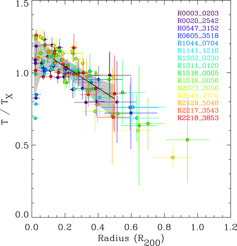
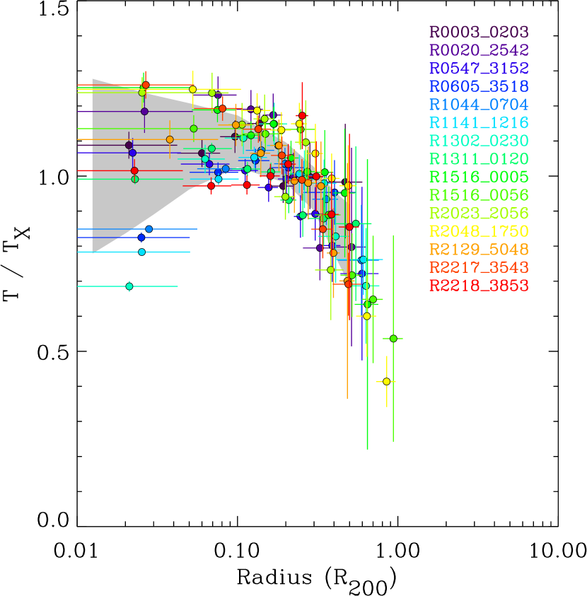
Figure 4: Scaled projected temperature profiles. Left panel: linear $x$-axis; right panel: logarithmic $x$-axis. The profiles have been normalised to the mean spectroscopic temperature in the $0.1\,R_{200}\leq r\leq 0.4\,R_{200}$ region, where $R_{200}$ has been determined iteratively using the $R$–$T$ relation of Arnaud et al. (2005). The shaded grey area corresponds to the region enclosed by the mean plus/minus the $1\sigma$ standard deviation. The solid line in the left-hand panel is the linear fit in the radial range $0.125<R_{200}<0.5$ detailed in Eqn. 1. (This figure is available in colour in the online version of the journal.)

We normalise the radial temperature profile of each cluster by a global temperature, $T_{X}$, which should be representative of the ‘virial’ temperature of the cluster. Strong cooling core clusters have central temperature decrements of up to a factor of three which, when combined with the $n_{e}^{2}$ dependence of the X-ray emission, means that average integrated temperatures of such systems can be biased. However, the cooling core region rarely extends beyond $\sim 0.1\,R_{200}$. In addition, our measured temperature profiles do not extend to much further than 1 Mpc even in the best cases, which corresponds to $\sim 60$ per cent of $R_{200}$ for a 5 keV cluster (Arnaud et al., 2005). We thus chose to use the overall spectroscopic temperature in the $0.1\,R_{200}\leq r\leq 0.4\,R_{200}$ region. We estimated this region in an iterative fashion, using the $R_{200}$–$T$ relation of Arnaud et al. (2005) and starting with the mean temperature from the measured temperature profiles. The measured values of $T_{X}$ are given in Table 1.

The resulting scaled temperature profiles are shown in Figure 4. It is obvious that, despite the large variety of objects in this sample, from strong cooling core objects to highly unrelaxed systems, there is some similarity in the temperature profiles; the profiles generally decline from the centre to the outer regions. As an initial measure of the scatter in scaled temperature profiles, we estimated the dispersion at various scaled radii in the range $0.0125$–$0.5\,R_{200}$. The shaded region in Fig. 4 shows the region enclosed by the mean plus/minus the $1\sigma$ standard deviation. Clearly the scatter increases towards the central regions. The relative dispersion in scaled profiles remains approximately constant at $\sim 10$ per cent beyond $0.1\,R_{200}$. In the core regions, however, this increases to $\sim 25$ per cent. Since the profiles have not been corrected for PSF and projection effects, this figure is likely a lower limit. In fact there is a clear difference between the cool core clusters, which have a large temperature drop toward the centre, and the non-cool core clusters, which generally have profiles which increase linearly or flatten toward the centre.

The largest cluster samples were assembled from ASCA and BeppoSAX (Markevitch et al. 1998 and De Grandi & Molendi 2002, respectively). More recent investigations with XMM-Newton (Piffaretti et al., 2005) and Chandra (Vikhlinin et al., 2005) have allowed better constraints to be put on the form of the profiles of cool core clusters out to 0.4-$0.5\,R_{200}$. In Fig. 5 we show a comparison of our temperature profiles with those from ASCA, BeppoSAX and Chandra. We use the same average temperature as above to normalise the temperatures, but as in these previous works, we scale the radial coordinate to $R_{180}$ using the relation given in (Evrard et al., 1996). There is good agreement between the profiles measured with different instruments. There is a tendency for our temperature profiles to scatter around the upper edge of the envelope of the ASCA results. We note however that the same tendency is seen in the Chandra observations (see Fig. 16 of Vikhlinin et al., 2005).

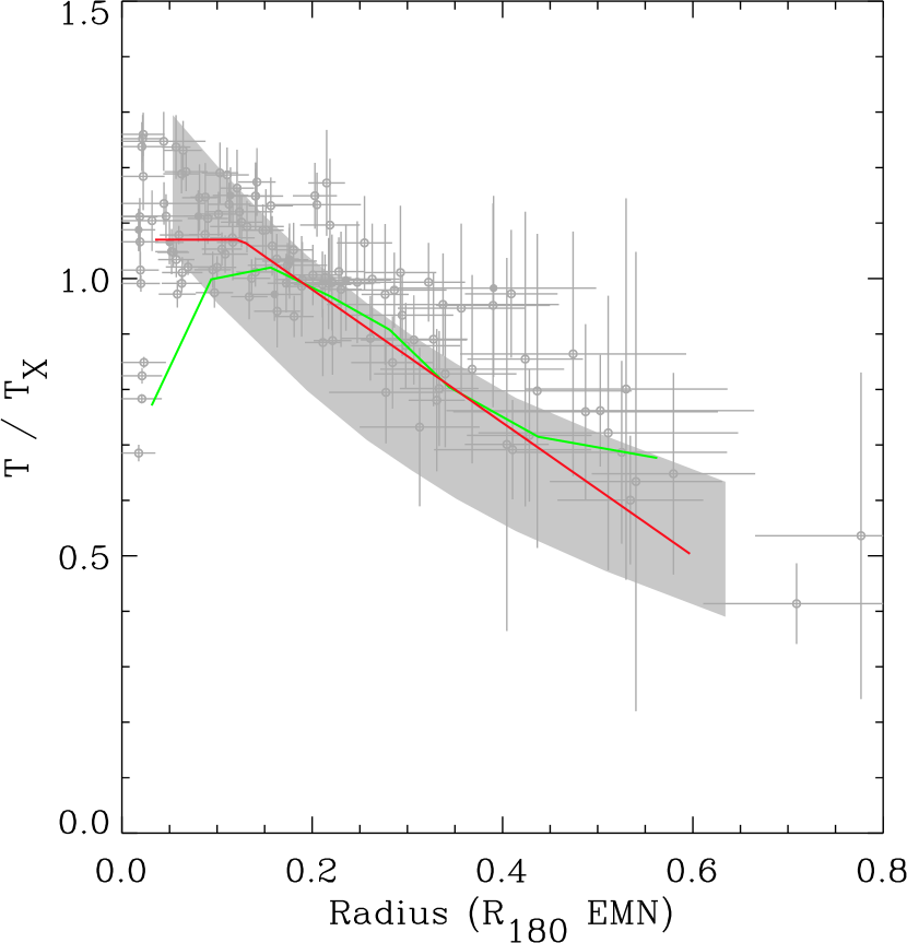
Figure 5: Scaled projected temperature profiles compared with the average profiles from ASCA (Markevitch et al., 1998, grey band), BeppoSAX observations of cooling core clusters (De Grandi & Molendi, 2002, green line), and Chandra observations of cooling core systems (Vikhlinin et al., 2005, red line). The observed profiles have been scaled using $R_{180}$ derived from the simulations of Evrard et al. (1996). (This figure is available in colour in the online version of the journal.)

It should be noted that the definitions of the global temperature and/or the virial radius often differ between samples, making exact comparison between different results rather difficult. We do not compare with the XMM-Newton results of Piffaretti et al. (2005) since their results are quoted for $R_{180}$ measured from the data, rather than derived from the relation of Evrard et al. (1996). We also note that the normalisation of the Piffaretti et al. (2005) profiles is $\sim 20$ per cent lower compared to our results and to those from other satellites. It is possible that this difference comes from their different definition of global temperature (Piffaretti et al. fit the emission-weighted bins outside the cooling core with a constant temperature). However, the general declining trend with radius is similar to their results.

Fitting the radial range $0.125<R_{200}<0.5$ with a simple linear model we find,

$$T/T_{X}=1.19-0.74R/R_{200}$$ (1)

for a fit with the BCES estimator. A linear least squares fit gives identical results.

4.2 Comparison with simulations

Negative gradients of the temperature profiles on scales $R>0.1\,R_{200}$ are naturally produced by cosmological hydrodynamical simulations of galaxy clusters, quite independent of the details of the physical processes included (e.g., Evrard et al., 1996; Lewis et al., 2000; Loken et al., 2002; Borgani et al., 2004; Kay et al., 2004). Markevitch et al. (1998) and De Grandi & Molendi (2002) compared observed temperature profiles from ASCA and Beppo-SAX data, respectively, to the results from non–radiative simulations by (Evrard et al., 1996) and found a reasonable agreement in the outer cluster regions. Loken et al. (2002) discussed a universal temperature profile in their simulated clusters, whose shape agrees well with observations outside the core regions. However, a number of authors have shown that including radiative cooling in simulations causes a substantial steepening of temperature profiles in the central cluster regions (e.g., Lewis et al., 2000; Valdarnini , 2003; Tornatore et al., 2003). The resulting temperature profiles are at variance with respect to the observed properties of cool core clusters (e.g., Borgani et al., 2004). This points towards the need to introduce a suitable energy feedback scheme to regulate gas cooling in the central regions (e.g., Kay et al., 2004).

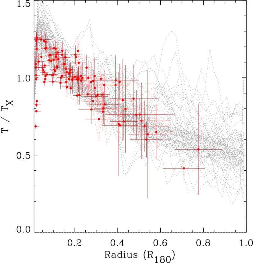
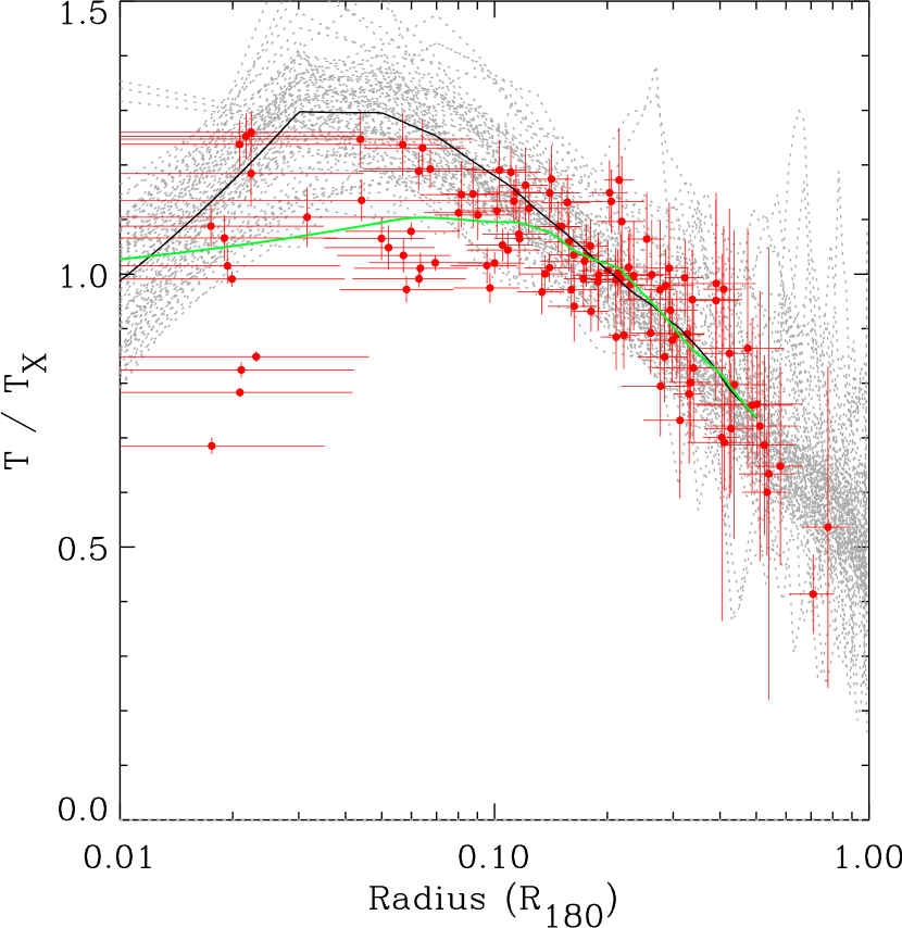
Figure 6: Scaled projected temperature profiles compared with the projected profiles of all clusters with ${\rm k}T>2$ keV from the simulations of Borgani et al. (2004). The mean profile of the observed and simulated profiles are shown by the black and green lines respectively. The observed profiles are scaled by the measured spectral temperature in the $0.1-0.4\,R_{200}$ region. The simulated profiles are scaled using the mean emission weighted temperature, with a further adjustment of 8 per cent to take into account the difference between the two definitions of global temperature used to scale the profiles. See text for details. (This figure is available in colour in the online version of the journal.)

In Figure 6 we show a comparison of the observed profiles with the projected simulated profiles of all clusters with ${\rm k}T>2$ keV from Borgani et al. (2004), in which the SPH code GADGET-2 (Springel, 2005) was used to simulate a concordance $\Lambda$CDM model ($\Omega_{M}=0.3,\Omega_{\Lambda}=0.7,\sigma_{8}=0.8,h=0.7$) within a box of $192\,h^{-1}$ Mpc on a side, using $480^{3}$ dark matter and an equal number of gas particles. The simulation included radiative cooling, star formation and galactic ejecta powered by supernova feedback. The observed profiles are scaled using the spectral temperature $T_{X}$, measured as described above in Sect 4.1. The simulated profiles were scaled using the emission weighted global temperature, with a further 8 per cent adjustment so that the normalisation in the $0.15<R_{200}<0.5$ region is the same as that of the observed profiles (this adjustment is necessary because the emission weighted global temperature is not the same as the measured spectral global temperature $T_{X}$). Three projections are shown for each cluster. The scatter in the simulated profiles is noticeable and comes from colder subclumps accreting onto the main cluster and shock fronts due to supersonic accretion. The simulated profiles decline continuously from a peak at about $0.05\,R_{180}$. The mean observed and simulated profiles are shown as black and green lines, respectively.

Table 3: Cluster power ratios, calculated in an aperture corresponding to $R_{500}$, estimated from the $R$–$T$ relation of Arnaud et al. (2005). Columns: (1) Cluster name; (2): $R_{500}$ in arcminutes; (3,5,7) power ratios; (4,6,8) $1\sigma$ errors on power ratios.

RXCJ	$R_{500}$	$P_{2}/P_{0}$	$\sigma_{P_{2}/P_{0}}$	$P_{3}/P_{0}$	$\sigma_{P_{3}/P_{0}}$	$P_{4}/P_{0}$	$\sigma_{P_{4}/P_{0}}$
0003+0203	$9\aas@@fstack{\prime}25$	$1.06\times 10^{-6}$	$3.67\times 10^{-8}$	$8.16\times 10^{-8}$	$1.16\times 10^{-8}$	$4.01\times 10^{-8}$	$4.66\times 10^{-9}$
0020-2542	$7\aas@@fstack{\prime}32$	$9.76\times 10^{-7}$	$3.11\times 10^{-8}$	$-3.48\times 10^{-9}$	$9.68\times 10^{-9}$	$-1.15\times 10^{-9}$	$4.35\times 10^{-9}$
0547-3152	$7\aas@@fstack{\prime}47$	$8.22\times 10^{-7}$	$1.92\times 10^{-8}$	$1.04\times 10^{-7}$	$6.10\times 10^{-9}$	$6.33\times 10^{-8}$	$2.50\times 10^{-9}$
0605-3518	$6\aas@@fstack{\prime}59$	$7.10\times 10^{-7}$	$9.90\times 10^{-9}$	$-2.70\times 10^{-9}$	$2.69\times 10^{-9}$	$2.25\times 10^{-9}$	$1.21\times 10^{-9}$
1044-0704	$5\aas@@fstack{\prime}91$	$1.64\times 10^{-6}$	$7.88\times 10^{-9}$	$-1.61\times 10^{-9}$	$2.18\times 10^{-9}$	$3.27\times 10^{-10}$	$8.32\times 10^{-10}$
1141-1216	$6\aas@@fstack{\prime}55$	$4.87\times 10^{-7}$	$1.28\times 10^{-8}$	$4.14\times 10^{-8}$	$3.69\times 10^{-9}$	$2.22\times 10^{-9}$	$1.58\times 10^{-9}$
1302-0230	$9\aas@@fstack{\prime}10$	$7.97\times 10^{-6}$	$4.40\times 10^{-8}$	$2.76\times 10^{-7}$	$1.31\times 10^{-8}$	$5.93\times 10^{-8}$	$5.88\times 10^{-9}$
1311-0120	$7\aas@@fstack{\prime}23$	$2.54\times 10^{-7}$	$4.35\times 10^{-9}$	$1.27\times 10^{-8}$	$1.05\times 10^{-9}$	$5.36\times 10^{-9}$	$4.90\times 10^{-10}$
1516+0005	$7\aas@@fstack{\prime}28$	$2.63\times 10^{-7}$	$2.64\times 10^{-8}$	$7.24\times 10^{-8}$	$7.97\times 10^{-9}$	$9.54\times 10^{-8}$	$3.35\times 10^{-9}$
1516-0056	$6\aas@@fstack{\prime}69$	$4.41\times 10^{-6}$	$6.54\times 10^{-8}$	$9.63\times 10^{-7}$	$2.20\times 10^{-8}$	$8.05\times 10^{-8}$	$9.08\times 10^{-9}$
2023-2056	$11\aas@@fstack{\prime}74$	$3.35\times 10^{-7}$	$1.22\times 10^{-7}$	$-3.43\times 10^{-8}$	$4.09\times 10^{-8}$	$4.80\times 10^{-8}$	$1.95\times 10^{-8}$
2048-1750	$6\aas@@fstack{\prime}08$	$5.89\times 10^{-6}$	$5.53\times 10^{-8}$	$2.97\times 10^{-7}$	$1.51\times 10^{-8}$	$1.46\times 10^{6}$	$6.70\times 10^{-9}$
2129-5048	$10\aas@@fstack{\prime}01$	$7.18\times 10^{-8}$	$6.68\times 10^{-8}$	$3.22\times 10^{-7}$	$1.94\times 10^{-8}$	$-5.76\times 10^{-9}$	$8.93\times 10^{-9}$
2217-3543	$6\aas@@fstack{\prime}18$	$5.33\times 10^{-7}$	$2.21\times 10^{-8}$	$3.25\times 10^{-8}$	$6.25\times 10^{-9}$	$9.83\times 10^{-9}$	$2.61\times 10^{-9}$
2218-3853	$7\aas@@fstack{\prime}28$	$5.28\times 10^{-6}$	$1.40\times 10^{-8}$	$3.65\times 10^{-8}$	$4.37\times 10^{-9}$	$1.68\times 10^{-8}$	$2.03\times 10^{-9}$

There is relatively good agreement in the external regions, with the simulated profiles reproducing the observed scatter. In the central regions the peak of the simulated temperature profiles lies at $\sim 0.04\,R_{180}$, in contrast to the observations, which show a less pronounced peak at $\sim 0.06\,R_{180}$, a point which is particularly evident from the mean profiles. In addition there appears to be considerably more dispersion in the observed profiles in the central regions. While admittedly our profiles are uncorrected for PSF and projection effects, we note that a similar difference in peak position (as compared to the simulations) is also evident when comparing with the Chandra results of Vikhlinin et al. (2005). Clearly, a more rigorous comparison would require estimating temperatures in the simulated clusters and rescaling their profiles in exactly the same manner as the data. Nevertheless, we believe that the agreement between simulated and observed clusters is quite good and lends support to the capability of numerical simulations to describe the global thermal structure of the ICM.

4.3 Dependence on cluster morphology/dynamical state

It is interesting to investigate whether there are correlations between the form of the temperature profile and the morphology or dynamical state of the cluster. To this end, we make a preliminary investigation using the power ratio method of Buote & Tsai (1995) to characterise the morpho-dynamical state of the objects in our sample.

Figure 7: Power ratios. The power ratios are computed in an aperture corresponding to $R_{500}$ estimated using the $R$–$T$ relation of Arnaud et al. (2005). See text for details.

4.3.1 Power ratio calculation

To obtain a quantitative estimate of substructure in the surface brightness distribution of the clusters, we applied the analysis method proposed by Buote & Tsai (1995). In this method, the projected mass distribution is associated with the X-ray surface brightness; a multipole expansion of the X-ray image then yields a similar expansion of the gravitational potential. The multipole analysis provides a measure of the ’power’ of each multipole component to the X-ray image of the cluster in absolute units. To obtain a measure that is independent of the cluster X-ray luminosity, the ’power’ terms are scaled by the zeroth order (monopole) moment and are consequently called ’power ratios’. The method was recently used to compare substructure in nearby and distant cluster samples observed with Chandra (Jeltema et al., 2005).

The method is applied within an aperture radius as described in Buote & Tsai (1995). We used a minimization of the first (dipole) moment to obtain an independent centering of the cluster emission within the aperture. The lowest order power ratios which are of interest for our study are $P_{2}/P_{0}$, $P_{3}/P_{0}$, and $P_{4}/P_{0}$, which correspond to the quadruple, the hexapole, and the octopole moments. Due to the nature of the moment functions, a large weight is given to the outer parts within the aperture, in particular for the higher moments. Thus the results depend somewhat on the choice of aperture. We have explored this effect with a range of aperture radii, results from which will be described in a future paper. For the purposes of this initial investigation, we estimate the power ratios within $R_{500}$, where this radius is estimated using the $R$–$T$ relation of (Arnaud et al., 2005).

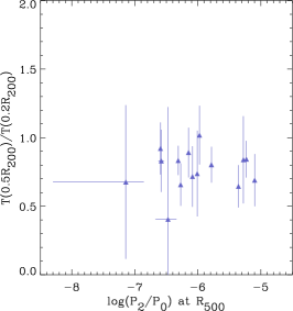
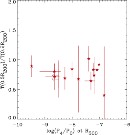
Figure 8: Scatter plots of $T(0.2_{R_{200}})/T(0.5_{R_{200}})$ (a measure of the temperature profile slope) with power ratio. There are no obvious correlations.

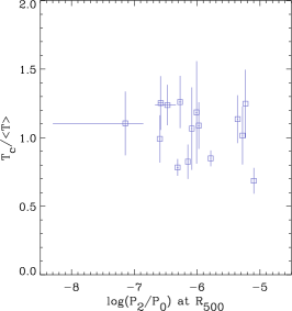
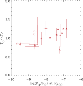
Figure 9: Scatter plots of the (projected) central temperature $T_{c}$ divided by the mean spectroscopic temperature in the $0.1\,R_{200}\leq r\leq 0.4\,R_{200}$ region (a measure of the central temperature dip) with power ratio.

Systematic effects and uncertainties for each power ratio were also taken into account. We created 1000 simulations of each cluster where the image pixels were azimuthally randomized around the predetermined cluster centre. The power ratio signal measured for these simulated clusters should be solely due to shot noise, providing a measure of the accuracy for rejection of the hypothesis that the cluster has no structure. We therefore subtract the mean of the simulated power ratio signal from the result obtained for the observed cluster and use the dispersion of the simulated results as an approximation of the error of the power ratio. We defer a more precise treatment to a forthcoming paper. The results shown in Fig. 7 demonstrate that we have sufficient photon statistics to produce robust results with small uncertainties, except for those cases where the clusters have a highly symmetric appearance. In general the results for the power ratios correspond very well to the visual impression of the cluster, where in particular $P_{2}/P_{0}$ can easily be identified with the cluster ellipticity. The parameter $P_{3}/P_{0}$ provides then the best measure for further substructure and since some ellipticity can be related to the quasi-equilibrium state of the cluster, the third moment provides often the strongest indication for a deviation from a relaxed dynamical state.

Power ratio values and $1\sigma$ errors are listed in Table 3. The power ratios for the clusters in our sample in general occupy a similar range of values to those derived for a nearby cluster sample by Jeltema et al. (2005). Plots of $P_{2}/P_{0}$ vs $P_{3}/P_{0}$, $P_{2}/P_{0}$ vs $P_{4}/P_{0}$ and $P_{3}/P_{0}$ vs $P_{4}/P_{0}$ are shown in Fig. 7. Of particular note is the strong correlation in $P_{4}/P_{0}$ vs $P_{3}/P_{0}$.

4.3.2 Preliminary comparison with power ratio

We can check to see if there are any correlations between the power ratio value and the shape of the temperature profile. We parameterise the outer temperature slope by measuring the ratio between the temperature at $0.5\,R_{200}$ and the temperature at $0.2\,R_{200}$ ($T(0.5_{R_{200}})/T(0.2_{R_{200}})$. These values are calculated by spline interpolation and are extrapolated if necessary. In Fig. 8, we show a scatter plot of the outer slope parameter and each of the power ratios. We then tested for correlations between $T(0.5_{R_{200}})/T(0.2_{R_{200}})$ and power ratio in the linear-log plane. We calculate the generalised Kendall’s $\tau$ correlation coefficient (Isobe et al., 1986), appropriate for censored data, for each scatter plot. The probability that a correlation is not present is 80, 66 and 88 per cent for $T(0.5_{R_{200}})/T(0.2_{R_{200}})$ vs $P_{2}/P_{0}$, $P_{3}/P_{0}$ and $P_{4}/P_{0}$, respectively. Given the wide range of morphologies present in the sample, the lack of significant correlation suggests that, in general, the morphology/dynamical state does not have a significant impact on the outer slope of the azimuthally averaged temperature profile, at least at the currently-available resolution.

Another interesting question is whether there is a correlation between the presence of a central temperature dip and the power ratio. In Fig. 9 we show a scatter plot of the ratio of the central temperature, $T_{c}$ (the temperature of the first bin in the temperature profile) to the mean spectroscopic temperature $T_{X}$, and each of the power ratios. Calculating the generalised Kendall’s $\tau$ correlation coefficient for each scatter plot, we find a probability that a correlation is not present of 55, 87 and 9 per cent for $T_{c}/T_{X}$ vs $P_{2}/P_{0}$, $P_{3}/P_{0}$ and $P_{4}/P_{0}$, respectively. Thus there is evidence for a weak correlation of central temperature drop with $P_{4}/P_{0}$, in the sense that clusters with smaller $P_{4}/P_{0}$ are more likely to have a central temperature drop. We do not yet have the full sample of clusters from which correlations can be derived, nor have the temperature profiles been corrected for PSF and projection effects, which will enhance the observed central gradients to some degree.

It should be noted that the spatial resolution of these and other recent temperature profiles, particularly at large radius, while much improved over results from previous satellites, is still the limiting factor when looking for correlations, or comparison between different cluster subsamples. This will also have a bearing on comparisons with numerical simulations.

5 Conclusions

We have used XMM-Newton observations of 15 clusters drawn from a statistically representative, luminosity-selected sample to investigate the behaviour of the temperature profiles. The clusters range from morphologically relaxed looking objects with strong central surface brightness peaks (e.g., RXC J1044 -0704), to diffuse structures with significant amounts of surrounding substructure (e.g., RXC J1516 +0056), and constitute a representative subsample. We find that, once scaled appropriately, the temperature profiles are similar in the radial range from $0.1\,R_{200}$ to $0.5\,R_{200}$, declining steadily from the central regions to the outer boundary of the measurements with a relative dispersion of $\sim 10$ per cent out to $0.5\,R_{200}$. The region interior to $0.1\,R_{200}$ is the region of greatest scatter in the scaled profiles: the relative scatter of $\sim 25$ per cent is likely a lower limit. A preliminary comparison with numerical simulations shows relatively good agreement outside $\sim 0.1\,R_{200}$, with all of the measured temperature profiles falling within the scatter of the simulated profiles.

Calculating power ratios for the sample, we investigate whether there are correlations between the power ratio measured in an aperture corresponding to $R_{500}$ and the shape of the temperature profile. We characterise the temperature profile shape in two ways: with the ratio $T(0.5\,R_{200})/T(0.2\,R_{200})$, a measure of the outer slope, and with the ratio $T_{c}/\langle T\rangle$, a measure of the central temperature drop. There is no obvious correlation of outer slope with power ratio; neither is there a correlation of central temperature dip with $P_{2}/P_{0}$ or $P_{3}/P_{0}$. There is evidence for a weak correlation of the central temperature dip with $P_{4}/P_{0}$. The analysis thus suggests that the outer slope of the temperature profile is not particularly sensitive to the morpho-dynamical state, although there may be some correlation with the existence of a central temperature drop. Further investigation with power ratios evaluated in other apertures, for the entire sample, should be undertaken before definitive conclusions can be drawm.

The overall conclusion from this work on a statistically representative sample indicates that clusters are a relatively regular population, at least outside the cool core regions, with the caveat that comparisons between samples or with simulations is limited by the available temperature profile resolution. The observed similarity in density (Neumann & Arnaud, 1999; Croston et al., 2006) and temperature profiles (Markevitch et al., 1998; De Grandi & Molendi, 2002; Piffaretti et al., 2005; Vikhlinin et al., 2005, this work) indicates both similarity in the underlying gravitational mass distribution (such as has already been seen in the X-ray mass profiles of morphologically relaxed clusters, e.g., Pointecouteau, Arnaud & Pratt 2005), and similarity in the entropy of the ICM (such as has been seen by e.g., Ponman, Sanderson & Finoguenov 2003; Pratt, Arnaud & Pointecouteau 2006). In this case a single integrated temperature, excluding the core region, should be a good proxy for the total mass. The observed regularity thus has important implications for the use of clusters as cosmological probes.

In future papers, we will reinvestigate the trends with the full sample, make maps of quantities such as temperature, entropy and pressure, and estimate the mass, baryon fraction and entropy in the clusters. A more extensive comparison with numerical simulations will also be undertaken.

Appendix A Individual cluster profiles

A.1 RXC J0003 +0203

RXC J0003 +0203, also known as Abell 2700, has an average temperature of ${\rm k}T=3.8$ keV and lies at $z=0.092$. The cluster presents a symmetric X-ray image but does not possess a strong central surface brightness peak. After renormalisation of the quiescent background, the spectra extracted in the external region ($r>11\arcmin$) can be adequately fitted with a MeKaL model at 0.23 keV with negative normalisation. An additional power-law is required for the EMOS2 and EPN spectra.

The temperature and metallicity profiles are shown in Fig. 10. The temperature profile is consistent with being isothermal at large radii, although given the $\sim 35\%$ uncertainties in the final bin, a decline cannot be ruled out. The metallicity profile is highly peaked, declining smoothly from $Z\sim 0.5Z_{\odot}$ in the central bin to $Z\sim 0.25Z_{\odot}$ at large radii. While the increase in metallicity towards the centre is reminiscent of a cooling core (De Grandi & Molendi, 2002), the temperature profile does not show a significant central decline, at least at the resolution of these data.

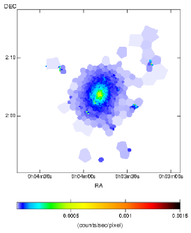
Figure 10: Image (left), temperature (middle) and abundance (right) profiles of RXC J0003 +0203. In this and the following images, the colour scale is square root with a maximum of 0.0015 counts per second (enabling easy comparison between images). The angular size of each image has been chosen to approximately match the virial radius of the cluster as determined from the average temperature $T_{X}$ (as defined in Sect. 4.1) and the $R$–$T$ relation of Arnaud et al. (2005). The horizontal line without errors in the abundance profile plots denotes the regions where the abundance was frozen. (Figures are available in colour in the online version of the journal.)

A.2 RXC J0020 -2542

Moderately luminous, lying at $z=0.141$ and with a temperature of ${\rm k}T=5.7$ keV, this cluster is also known as Abell 22. The X-ray image is highly disturbed, with a prominent surface brightness edge to the N, and an emission extension to the S. The overall X-ray emission is aligned approximately in the direction of the line joining the two brightest cluster galaxies. The annular regions were centred on the surface brightness peak, which lies on the surface brightness edge and corresponds to the position of the BCG. The residual spectrum shows negative residuals and is adequately described with a combination of a MeKaL model at 0.10 keV with negative normalisation, with an additional power-law component for the EMOS2 and EPN.

The temperature profile (Fig. 11) shows a prominent decline with radius. The abundances are roughly flat but became unconstrained at only $\sim 400$ kpc from the centre and were frozen thereafter.

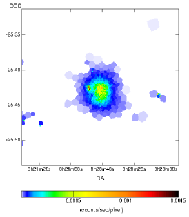
Figure 11: RXC J0020 -2542.

A.3 RXC J0547 -3152

Also known as Abell 3364, this luminous cluster lies at $z=0.148$ and has an average temperature of ${\rm k}T=6.6$ keV. The X-ray image shows a bright, offset core, with obvious surface brightness edges to the NW and SE. After renormalisation, the spectrum of the external region shows negative residuals below $\sim 1$ keV. These are adequately described with a MeKaL model with negative normalisation and a temperature of 0.24 keV. An additional power-law component is needed to fully describe the EPN spectrum (see Fig. 2).

The temperature profile declines monotonically, from ${\rm k}T\sim 7$ keV to ${\rm k}T\sim 4.5$ keV, from the centre to the largest radii at which we can measure the temperature. The metallicity profile declines from $Z\sim 0.4Z_{\odot}$ to $Z\sim 0.2Z_{\odot}$ between $0<r<300$ kpc, but then increases once more to the central value at $r\sim 600$ kpc. The metallicity trends may be connected to the disturbed nature of the cluster.

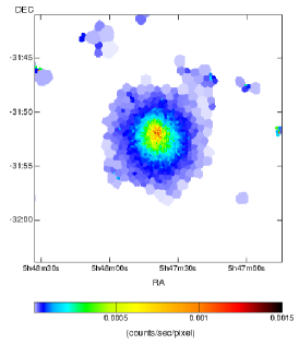
Figure 12: RXC J0547 -3152.

A.4 RXC J0605 -3518

Lying at $z=0.14$, with an average temperature of ${\rm k}T=4.7$ keV, this cluster is also known as Abell 3387. It is highly symmetric, presenting a strongly-peaked central surface brightness and no visible substructure. The residual spectrum is well described with a MeKaL model with negative normalisation and a temperature of 0.26 keV. An additional power-law component is necessary for a full description of the EPN data.

The temperature profile (Fig. 13) rises from the central regions to a peak at $R\sim 200$ kpc, after which there is a gentle decline. The abundance profile declines smoothly from $\sim 0.6\,Z_{\odot}$ in the central regions to $\sim 0.2\,Z_{\odot}$ at $R>500$ kpc. The general behaviour of the temperature and abundance profiles is very reminiscent of the Chandra temperature profiles of cool core clusters derived by Vikhlinin et al. (2005).

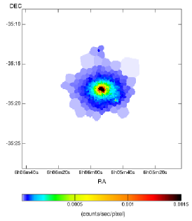
Figure 13: RXC J0605 -3518.

A.5 RXC J1044 -0704

RXC J1044 -0704, also known as Abell 1048, lies at $z=0.13$. It has an average temperature of ${\rm k}T=3.6$ keV and although slightly elliptical, is another symmetric cluster with a strongly-peaked central surface brightness. The residual spectrum is negative in the 0.5-1.0 keV band, indicating oversubtraction of the background in this band. The residual spectrum can be fitted with a MeKaL model at 0.26 keV with negative normalisation. An additional power-law component improves the fit to the EPN data.

The temperature and abundance profiles (Fig. 14) are once again reminiscent of those of other cool core clusters. The temperature climbs to a peak at $R\sim 200$ kpc and declines thereafter, while the abundance profile declines from the central regions to the outskirts (although in this case the decline is not smooth).

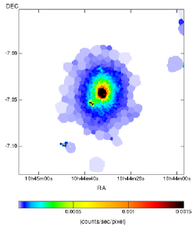
Figure 14: RXC J1044 -0704.

A.6 RXC J1141 -1216

This highly symmetric cluster at $z=0.12$ exhibits strongly peaked central emission. The cluster is also known as Abell 1348 and has an average temperature of ${\rm k}T=3.6$ keV. The residual spectrum shows negative residuals and is well fitted with a simple MeKaL model with negative normalisation and a temperature of 0.27 keV.

The temperature and abundance profiles shown in Fig. 15 are very similar to those of the previous two clusters. The central temperature dip is associated with an abundance enhancement; the temperature peaks around 200 kpc and declines gently thereafter. The abundance declines smoothly from the centre to the external regions.

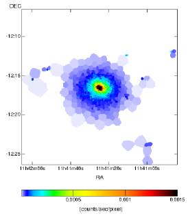
Figure 15: RXC J1141 -1216.

A.7 RXC J1302 -0230

Also known as Abell 1663, this is a symmetric looking cluster at ${\rm k}T=3.6$ keV lying at $z=0.085$. It has a strong central emission peak. The residual spectrum of the external region ($r>11\arcmin$) can be characterised with a MeKaL model at 0.27 keV with negative normalisation. An additional power law component improves the fit for the EMOS2 and EPN spectra.

The temperature and abundance profiles (Fig. 16) are very characteristic of cooling core clusters. Compared to similar clusters in this sample, however, RXC J1302 -0230 is characterised by a particularly steep central temperature drop, and a similarly steep increase of metallicity towards the central regions.

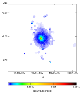
Figure 16: RXC J1302 -0230.

A.8 RXC J1311 -0120

This extremely symmetric cluster lying at $z=0.183$ is the well-known lensing cluster Abell 1689. This is the most luminous cluster in the present sample, which is reflected by its particularly high temperature (${\rm k}T=8.5$ keV). The residual spectrum of the external region ($r>11\arcmin$) shows a positive excess which is well modelled by a MeKaL model at 0.19 keV. An additional power-law component improves the fit for the EPN detector.

The temperature and abundance profiles (Fig. 17) are not characteristic of cooling core clusters, however. While there is a central temperature drop, it is not nearly as steep as that displayed by other cool core clusters in this sample. Furthermore, the abundance profile does not show a central peak. The temperature and abundance profiles we have derived are in good agreement with those derived (from the same XMM-Newton data) by Andersson & Madejski (2004). Girardi et al. (1997) use galaxy velocity date to describe this cluster as a line of sight merger. This may explain why the clusters is quite symmetric but does not appear to possess a strong cooling core.

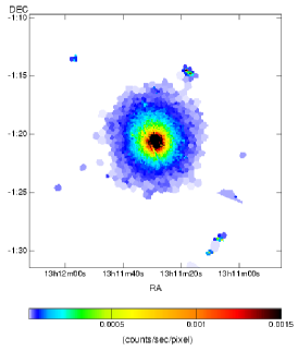
Figure 17: RXC J1311 -0120.

A.9 RXC J1516 +0005

Also known as Abell 2050, this moderate temperature (${\rm k}T=4.6$ keV) symmetric looking cluster lying at $z=0.120$ does not, however, exhibit peaked central emission. The external residual spectrum, accumulated from events from beyond $12.5\arcmin$ from the cluster centre exhibits an excess of counts at $E<1$ keV and is adequately fitted with a MeKaL model at 0.25 keV. An additional power law component improves the EPN fit.

The temperature profile of this cluster (Fig. 18) shows no sign of cool core emission, declining linearly from the centre to the external regions. As expected, the abundance profile is consistent with being flat at $Z\sim 0.3\,Z_{\odot}$ out to 500 kpc (the maximum radius at which we can measure abundances).

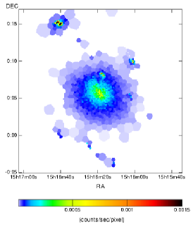
Figure 18: RXC J1516 +0005.

A.10 RXC J1516 +0056

A moderate temperature (${\rm k}T=3.75$ keV) cluster lying at $z=0.120$, RXC J1516 +0056 is also known as A2051. The X-ray image presents quite a lot of structure, with several possible subclumps at the outskirts of the object. These subclumps were excluded from the annuli used to determine the temperature profile. The background subtracted spectrum of the external region is well fitted with a single MeKaL model at 0.25 keV, with positive normalisation.

The temperature and abundance profiles are shown in Fig 19. The temperature profile is flat in the inner 400 kpc, but declines by $\sim 50$ per cent at the radius of maximum detection. The abundance profile is consistent with being flat out to the radius of maximum detection.

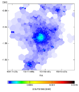
Figure 19: RXC J1516 -0056

A.11 RXC J2023 -2056

Also known as S868, lying at $z=0.056$, this is the lowest temperature cluster in the present sample (${\rm k}T=2.7$ keV). The object has a fairly regular appearance, but no strong evidence for a cooling core. The background subtracted external region spectrum is well described by a MeKal model with positive normalisation and a temperature of 0.23 keV. An additional power law component improves the fit of the EPN data.

The temperature profile of the cluster, shown in Fig 20 is flat in the inner 100 kpc, after which there is a decline. The abundance profile declines smoothly in power law fashion from a peak of $Z=0.5Z_{\odot}$ in the centre to about half that value at the outskirts.

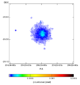
Figure 20: RXC J2023 -2056.

A.12 RXC J2048 -1750

With a temperature of ${\rm k}T=4$ keV and lying at $z=0.085$, RXC J2048 -1750 presents a fairly disturbed appearance. The background subtracted spectrum of the region external to the cluster emission can be fitted with a simple thermal model at 0.20 keV, with positive normalisation.

The temperature profile of the cluster (Fig. 21) declines linearly, by more than a factor of two, from the centre to the external regions. The abundance profile is very poorly constrained, and we can only measure the three inner bins.

Figure 21: RXC J2048 -1750.

A.13 RXC J2129 -5048

A moderate temperature (${\rm k}T=3.8$ keV) cluster also known as A3771, RXC J2129 -5048 lies at $z=0.08$. The X-ray image is disturbed, with a distinct elongation in emission from the centre towards the NE. The background subtracted spectrum of the external region can be fitted with a thermal model at ${\rm k}T=0.33$ keV with an additional power law improving the fit in all three cameras.

The temperature profile of the cluster (Fig. 22) is relatively flat in the inner 200 kpc or so, but declines beyond this. The abundance profile is relatively poorly constrained, but is consistent with being flat at an average of $Z\sim 0.35Z_{\odot}$.

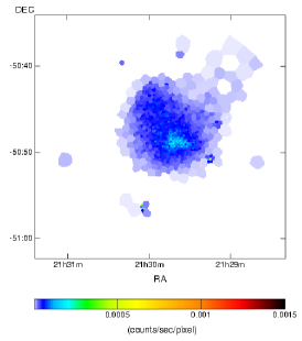
Figure 22: RXC J2129 -5048.

A.14 RXC J2217 -3543

One of the more distant clusters in the sample, having an average temperature of ${\rm k}T=4.6$ keV and lying at $z=0.148$, RXC J2217 -3543 is also known as A3584. The X-ray image is quite compact and symmetric, although the cluster does not present strongly-peaked core emission. The spectrum of the background subtracted external region presents strongly negative residuals below 1 keV and can be fitted with a thermal model at 0.65 keV, with negative normalisation.

The temperature profile shown in Fig. 23 declines linearly from the peak of 5.5 keV at the centre to 3 keV at the maximum radius at which we can measure the temperature. The abundance profile does not show any trends with radius.

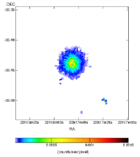
Figure 23: RXC J2217 -3543.

A.15 RXC J2218 -3853

RXC J2218 -3853 is also known as A3856, has an average temperature of ${\rm k}T=5.8$ keV and lies at $z=0.09$. The X-ray image is elliptical, presenting an elongation in the SE-NW direction. The background subtracted spectrum of the external region is well fitted with a thermal model at 0.26 keV, with an additional power law component improving the fit for all three cameras.

The temperature profile (Fig. 24) is flat in the inner regions, rises to a peak at $\sim 400$ kpc, and then declines (although not significantly). The abundance profile is consistent with being flat at an average of $Z=0.3Z_{\odot}$ out to 400 kpc, the detection limit.

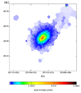
Figure 24: RXC J2218 -3853.