Mapping population synthesis event rates on model parameters II: Convergence and accuracy of multidimensional fits

Abstract

Binary population synthesis calculations and associated predictions, especially event rates, are known to depend on a significant number of input model parameters with different degrees of sensitivity. At the same time, for systems with relatively low formation rates, such simulations are heavily computationally demanding and therefore the needed explorations of the high-dimensional parameter space require major – often prohibitive – computational resources. In the present study, to better understand several key event rates involving binary evolution and binaries with two compact objects in Milky Way-like galaxies and to provide ways of reducing the computational costs of complete parameter space explorations: (i) we perform a methodical parameter study of the StarTrack population synthesis code ; and (ii) we develop a formalism and methodology for the derivation of multi-dimensional fits for event rates. We significantly generalize our earlier study, and we focus on ways of thoroughly assessing the accuracy of the fits. We anticipate that the efficient tools developed here can be applied in lieu of large-scale population calculations and will facilitate the exploration of the dependence of rate predictions on a wide range binary evolution parameters. Such explorations can then allow the derivation of constraints on these parameters, given empirical rate constraints and accounting for fitting errors. Here we describe in detail the principles and practice behind constructing these fits, estimating their accuracy, and comparing them with observations in a manner that accounts for their errors.

1. Introduction

Models for binary stellar evolution and population syntheses are necessary to provide quantitative theoretical predictions for the relative likelihood of assorted events involving the evolution of binary stars. The resulting predictions are particularly critical when no empirical estimates exist for topics of immediate astrophysical interest, such as mergers of double-compact object (DCO) through the emission of gravitational waves. The most practical and widely applied binary population synthesis codes available in the community – such as the StarTrack code described in Belczynski et al. (2002) and significantly updated in Belczynski et al. (2006a); the BSE code, described in Hurley et al. (2002); the SeBa code described in Portegies Zwart & Verbunt (1996); and the StarFaster code described in Fryer et al. (1998) – rely on a large set of fairly simple parameterized rules to characterize many complex and often ill-understood physical processes. Unfortunately, current binary population synthesis codes are greatly and often forbiddingly computationally demanding (depending on their level of sophistication): even with substantial simplifications, exploring the entire parameter space relevant to the simulations is beyond present-day computational capability.

However, observational information can provide us with constraints that help us improve our understanding of massive binary evolution. For example, pulsar searches continue to discover and refine observations of isolated pulsars and new binary pulsar systems; e.g., see Lorimer (2005) for a review. Specifically, the samples of binary pulsars with neutron star and relatively massive white dwarf companions have been used for a statistical derivation of empirical rate estimates for their formation (most recently see Kim et al. (2003), Kim et al. (2004), Kalogera et al. (2005) and references therein). Additionally, many ground-based gravitational wave detectors now operating at or near design sensitivity (i.e., LIGO, GEO, TAMA) are designed to detect the late stages of double compact object (DCO) inspiral and merger. Based only on early-stage data, these instruments have already provided conservative upper limits to certain DCO merger rates (see,e.g. Abbott et al., 2005b, a). With LIGO now very close to design sensitivity, a year of LIGO data could definitively exclude (and even possibly confirm) the most optimistic theoretical predictions for BH-BH merger rates (see, e.g. O’Shaughnessy et al., 2005a, for a range of BH-BH merger rates arising from binary evolution in Milky Way-like galaxies). Thus, gravitational-wave based upper limits (and, eventually, detections) will shortly provide constraints on theoretical models of DCO formation.

Faced with the availability of empirical rate constraints, and yet at first unable to quantitatively impose them on population synthesis predictions because of the extremely limited exploration of the multi-dimenional parameter space, O’Shaughnessy et al. (2005a) realized that any single unambiguous population synthesis prediction could be sampled loosely and then fit over the most sensitive population synthesis parameters. In the same study, we also presented a technique to accelerate the synthesis code used (StarTrack) to study a single target subpopulation, which we called “partitioning”: we used experience gained from prior simulations to reject binary parameters highly unlikely to produce the current event of interest. O’Shaughnessy et al. (2005b) first applied these early fits to allow a direct comparison between StarTrack-produced population synthesis predictions and the observed formation rate for NS-NS binaries. Though only a small fraction ($2\%$) of StarTrack models appeared consistent with the constraints, conceptual challenges with seven-dimensional visualization prevented O’Shaughnessy et al. (2005a) from clearly describing the constraint-satisfying region. A forthcoming paper, O’Shaughnessy et al. (2007b) will significantly extend that earlier preliminary analysis, adding significantly more observational constraints as well as a clearer investigation of the constraint-satisfying models.

In this paper, we extend and generalize the analysis of O’Shaughnessy et al. (2005a), and we present a thorough discussion of our much-updated and vastly larger population synthesis archive (§2) and particularly of the fitting methods we employ to extract predictions and assess their uncertainties and quality (§3). Because several imporant and yet not immediately obvious pitfalls must be identified avoided when constructing, testing, and applying fits, in this paper we provide a thorough and pedagogical discussion of our fitting method and philosophy. For example, we explain how systematic fitting errors that were ignored in O’Shaughnessy et al. (2005b) can limit our ability to constrain the merger rates in the Milky Way. In a companion paper (O’Shaughnessy et al., 2007b) we explore the astrophysical applications of these fits, emphasizing their use in deriving empirical constraints on population syntheses and rate predictions.

Though we develop the fitting formulation specifically for the results of the StarTrack code, the methods described in this paper can be applied to any family of population synthesis simulations. For this reason, we survey the physics underlying the StarTrack model only in our companion paper O’Shaughnessy et al. (2007b), in which these fits are used to cover the parameter space and apply empirical rate constraints from supernovae and binary pulsars.

2. Population synthesis archives

Population synthesis simulations can be extremely computationally demanding: even though StarTrack can fully evolve roughly $10^{3}$ binaries of interest per CPU-hour with modern-day processors, because some double compact objects form very infrequently (e.g., black holes, which occur roughly once every $\sim 10^{-4}$ binaries evolved), a representative sample of stellar systems often contains $10^{4.5}-10^{6.5}$ binaries and requires hundreds of CPU hours to complete. Additionally, since population synthesis rate predictions depend delicately on model parameters, the computation time needed to build up a sufficiently representative collection of stellar systems – one where some event of interest occurs many times – varies considerably depending on astrophysical assumptions. Given the prohibitive computational demands of a brute-force approach, we took advantage of several simplifications originally developed in O’Shaughnessy et al. (2005a) to assemble our archive of roughly 3000 population synthesis simulations, upon which our fits our predicated. In this section we briefly describe how those archives were generated and how we identify and extract event rates for several processes of interest.

2.1. StarTrack population synthesis code

We estimate formation and merger rates for several classes of double compact objects using the StarTrack code first developed by Belczynski et al. (2002) [hereafter BKB] and recently significantly updated and tested as described in detail in Belczynski et al. (2006a). Like other population synthesis codes, StarTrack evolves some number $N$ binaries from their birth (drawn randomly from specified birth distributions) to the present, tracking the stellar and binary parameters. Because binaries without any high-mass components cannot produce black holes or neutron stars, we configured StarTrack to simulate only those binaries whose heaviest initial component mass $m_{1}$ was greater than $4M_{\odot}$. In effect, the small number $N$ of binaries simulated mimic the results of a much larger simulation of size $N_{eff}$ in which $m_{1}$ can take on any value from the hydrogren burning limit ($0.08M_{\odot}$) to the maximum initial stellar mass we allow ($150M_{\odot}$):

$$N_{eff} = N/\int_{4M_{\odot}}^{150M_{\odot}}dm\;\phi(m)\simeq 131N$$ (1)

based on a broken Kroupa initial mass function $\phi(m)\propto m^{-1.3}$ if $m\in[0.08,0.5]M_{\odot}$, $\propto m^{-2.2}$ if $m\in[0.5,1]M_{\odot}$, and $\propto m^{-2.7}$ if $m>1M_{\odot}$. In turn, a simulation of $N_{eff}$ stellar systems can be scaled up to represent the $N_{g}$ stellar systems in the Milky Way. The number of stellar systems $N_{g}$ in the Milky Way (and thus the normalization of population synthesis simulations) can be estimated in many ways, depending on the observational inputs used; for the purposes of this paper, we estimate $N_{g}$ from the average number of binary systems formed through steady star formation over $T=10\,{\rm Gyr}$ of star formation at $\dot{M}\simeq 3.5M_{\odot}\,{\rm yr}^{-1}$ (Rana, 1991; Lacey & Fall, 1985):

$$N_{g} = \frac{\dot{M}T}{\left<m_{1}+m_{2}\right>}=\frac{\dot{M}T}{\left<m_{1}\right>\left(1+f_{b}\left<m_{2}/m_{1}\right>\right)}$$

$$\simeq 7.6\times 10^{10}\left(\frac{T}{10{\rm Gyr}}\right)\frac{1}{1+f_{b}\left<m_{2}\right>/\left<m_{1}\right>}$$

where $f_{b}$ is the binary fraction and $\left<m_{2}\right>/\left<m_{1}\right>$ is the ratio of average masses of the companion and primary, respectively. The proportionality constant $s\equiv N_{g}/N_{eff}$ needed to scale the results of our simulations up to the universe is therefore

$$s \equiv N_{g}/N_{eff}$$

$$= 5.9\times 10^{8}N^{-1}(T/10{\rm Gyr})\frac{1}{1+f_{b}[\left<m_{2}\right>/\left<m_{1}\right>]}$$

Note that parameters of the population synthesis model such as $f_{b}$ and $\left<m_{2}\right>/\left<m_{1}\right>$ influence the result at best by $O(50\%)$. These scaling relations allow us to estimate the merger rate implied by simulations ($R$) via a surrogate ($\tilde{R}$) based on the number $n$ of merger events seen in simulation:

$$\tilde{R} \equiv sn/T=7.6\times 10^{-3}\frac{n}{N}\frac{\dot{M}}{\left<m_{1}+m_{2}\right>}$$

$$\simeq 0.059{\rm yr}^{-1}\frac{n}{N}\frac{1}{1+f_{b}[\left<m_{2}\right>/\left<m_{1}\right>]}$$

[Unless otherwise noted, “tilde” quantities refer to estimates for the corresponding “normal” quantity for one individual simulation, based on only information from that one simulation.]

Given unlimited computational resources, this simulation could be repeated many times to measure the merger rate $R$ implied by this model to any accuracy desired, or equivalently measure the average number $\mu$ of of merger events expected from this simulation

$$\mu\equiv RT/s\,.$$ (5)

In practice, each simulation is performed once; therefore, the simulated number of merger events ($n$) is only statistically correlated to the average number of events expected ($\mu$), with relative probabilities $p(n|\mu)$ of any one simulation producing $n$ events given by the Poisson distribution

$$p(n|\mu)=\frac{\mu^{n}}{n!}e^{-\mu}\;.$$ (6)

On average our estimates of the $\tilde{R}=sn/T$ and equivalently of the number of events $\tilde{\mu}=n\;$ will agree with the true properties of the underlying simulation: averaging over many trials, $\left<\tilde{R}\right>=R$ and and $\left<\tilde{\mu}\right>=\mu$. However, an estimate based on any one specific simulation should differ from the mean by a characteristic relative amount

$$\sqrt{\left<(\log\tilde{R}-\log R)^{2}\right>} = \sqrt{\left<(\log\tilde{\mu}-\log\mu)^{2}\right>}$$

$$\simeq 1/\sqrt{\mu}\ln(10)\simeq 1/\sqrt{n}\ln(10)$$

2.2. Parameters varied in archives

Our extensive experience in modeling of binary compact objects with StarTrack clearly indicates that there are seven parameters that strongly influence compact object merger rates (see e.g., Belczynski et al. (2002)): the supernova kick distribution (3 parameters $\sigma_{1,2}$ and $s$ describing a superposition of two independent maxwellians), the massive stellar wind strength $w$ (1), the common-envelope energy transfer efficiency $\alpha\lambda$ (1), the fraction of mass accreted by the accretor in phases of non-conservative mass transfer $f_{a}$ (1), and the binary mass ratio distribution, as described by a negative power-law index $r$ (1). We allow the dimensionless parameters $\alpha\lambda,f_{a}$, $w$ and $s$ to run from 0 to 1; the dimensionless $r$ can be between $0$ and $3$; and finally we vary the dispersion of either component of a bimodal Maxwellian $\sigma_{1},\sigma_{2}$ from 0 to 1000 km/s. Additionally, motivated by recent observations suggesting pulsars with masses near $2M_{\odot}$ (see,e.g. Nice et al., 2005; Splaver et al., 2002), we assume the maximum neutron star mass to be $2.5M_{\odot}$.

To improve our statistics, we combine results from several different databases of simulations. The most extensive database samples $\sigma_{1}\in[200,1200]$ and $\sigma_{2}\in[0,200]$ very densely and was developed by O’Shaughnessy et al. (2005a) and O’Shaughnessy et al. (2005b). A second archive, significantly less dense due to computational resource limitations, allows both dispersions to run uniformly from 0 to 1000 km/s. [Additional archives include, for example, a set chosen to better-sample kick parameters that best correspond to observations of pulsar proper motions Arzoumanian et al. (1999); Hobbs et al. (2005).] Consequently, as shown in Figure 1, our archived results do not uniformly sample the kick-related parameters through this range. This irregular sampling has two effects. First, having irregular sampling of the model parameters effectively corresponds to imposing non-flat priors on these parameters and hence biasing the resulting distribution function of merger rates that come directly from the database of runs; see Appendix A and in particular Figure 6. Therefore it is even more important to develop the fits, which then allow us uniform sampling of the parameter space, and hence the derivation merger rate distributions assuming flat priors, as our intention is. Second, certain kick combinations are relatively undersampled, which likely plays a role in the relatively poor global convergence of fits for physical parameters, as described in § 4. Nonetheless, our sampling rather thoroughly explores the most physically likely regimes suggested by Hobbs et al. (2005) and Arzoumanian et al. (1999).

Figure 1.— Scatter plot of the two bimodal kick velocity dispersions $\sigma_{1}$, $\sigma_{2}$ for the population synthesis archives used to evaluate the merger rate of NS-NS binaries [denoted NSNS(m)]. The strong bias is introduced by incorporating high-density and computationally expensive simulations from O’Shaughnessy et al. (2005a) and O’Shaughnessy et al. (2005b).

2.3. Event identification

Most events of physical interest are uniquely and fairly unambiguously identifiable within the code. Type II and Ib/c supernovae events are distinguished by the presence or absence of a hydrogen-rich envelope at the supernova event. We also record DCOs which merge, so we can unambiguously determine the number of BH-BH, BH-NS, NS-NS, and WD-NS merger events which occur in a simulation. [These event classes will be denoted BHBH(m), BHNS(m), NSNS(m), and WDNS(m) for brevity henceforth.] Since the code also tracks binary eccentricity, for example, we can identify those WD-NS binaries which end their evolution with a non-zero eccentricy [denoted WDNS(e)].

When constructing our archived population synthesis results, we do not record detailed information about the nature and amount of any mass transfer onto the first-born NS. We therefore cannot determine the degree to which pulsars are recycled. However, we do record whether any mass transfer occurs. Thus for the purposes of identifying a class of potentially recycled (“visible”) wide NS-NS binaries [denoted NSNS(vw)], we assume any system undergoing non-CE mass transfer recycles its NS primary.

2.4. Practical Archive Generation and Resolution, with Partitions and Heterogeneous Targets

The accuracy to which each population synthesis event rate prediction is known, $\sim 1/\sqrt{n}$, is uniquely set by the number of events $n$ seen within that simulation. For this reason, O’Shaughnessy et al. (2005a) (i) designed their population synthesis runs to continue until a fixed number of events were seen and (ii) used results only from such targeted simulations, where a minimum number of events was guaranteed. In contrast in this study, given limited computational resources and a wide range of targets for which predictions are needed, we extract all possible information from each simulation: whenever possible, we make an estimate of each event rate of interest.

However, it is important to note that most of our simulations employ some degree of accelerating simplification which can bias estimates. To give the most extreme example: the most accurate estimates for the BH-BH merger rate come from population synthesis runs which evolve only a subset of possible progenitor binaries by using partitions. This subset has been shown to include the progenitors of the vast majority of BH-BH binaries, but very few progenitors of NS-NS binaries and other less massive DCOs (for more information, see O’Shaughnessy et al., 2005a, ; we continue to employ the same partition they devised). Similarly, the vast majority of simulations used to study NS-NS event rates (i) use a similar partition to reduce contamination from white dwarf binaries and (ii) terminate the evolution of any binary immediately after any WD forms. These strong biases make data from these two types of simulations inappropriate for use in, for example, estimating the WD-NS merger rate. For this reason, the number of population synthesis archives $N$ available to make predictions varies significantly across the various target event types; see Table 2.

Furthermore, the accuracy each simulation can provide varies considerably: unlike earlier studies, the number of event samples $n$ in each archive is not guaranteed to be greater than a minimum value. However, usually we have at least one event for each event type: $N_{s+}$, the number of unbiased population synthesis results containing one or more events is usually very close to $N_{s}$, the total number of unbiased population synthesis simulations available. And in most cases a significant proportion of our sample contains enough events to determine the rate to better than $30\%$ (i.e., $n\geq 10$).

3. Fitting: Principles and Tests

Given the prohibitive computational demands of direct population synthesis simulations described in § 2, we use fits based on archived results of population synthesis runs as a surrogate for repeated detailed simulations. Confidence in our results is therefore tied intimately to confidence in the quality of these fits. However, even low order fits in seven dimensions involve many parameters: to fit any nontrivial function, we must fit roughly a handful of data points per parameter. To build confidence, we must show that the fit order chosen adequately describes the data without overfitting. More delicately, since these fits are used in the derivation of empirical constraints on the population synthesis models in our companion paper (O’Shaughnessy et al., 2007b), we must also be able to show that the key end product, the ”constraint-satisfying model region” does not depend sensitively on the fit details or on random accidents in the data (i.e., any different Monte Carlo realization of our simulations should yield the same result). Finally, we note that our companion paper (O’Shaughnessy et al., 2007b) will impose four independent constraints. In order to have more than $90\%$ confidence that all models that satisfy all constraints are indeed inside the intersection of the four constraint-satisfying regions, we must at a minimum show that each individual constraint-satisfying prediction contains more than $0.90^{1/4}\simeq 0.974$ of the models that truly satisfy that constraint.

3.1. One-Dimensional Model

Though we intend to build confidence explicitly in our ability to make predictions on the basis of seven-dimensional fits, some of the required principles, notation, and tools are best illustrated through a one-dimensional example. Thus in this section we explore an arbitrarily-chosen but known “population synthesis” model. Depending on one real parameter $x$ with $0\leq x\leq 1$, this model on average will produce $\mu(x)$ merger events out of $N=10^{5}$ binaries, with $\mu(x)$ chosen arbitrarily as

$$\mu(x) \equiv 10^{M(x)}=5+20x^{2}\;.$$ (8)

Specifically, in this model we assume: all stars are born in binaries ($f_{b}=1$); that the smaller companion star has mass randomly distributed from the hydrogen burning limit to the primary’s mass, corresponding to $\left<m_{2}\right>/\left<m_{1}\right>=0.5$; and that star formation extends over an interval $T=10\,{\rm Gyr}$. Under these specific circumstances, as discussed in §2 [Eqs. (5,2.1)], a model which produces $\mu(x)$ events on average out of $10^{5}$ binaries corresponds to a merger rate

$$R(x) = s\mu(x)/T$$ (9)

$$\simeq 4\times 10^{-7}\mu(x)\,{\rm yr}^{-1}\;.$$ (10)

An individual simulation of this model will produce some number $n$ of events, with $n$ statistically related to $\mu(x)$ via the Poisson distribution [Eq. (6)].

To estimate the merger rate as a function of $x$, we perform several simulations ($N_{s}=11$) using different parameter values $x=x_{\alpha}=(\alpha-1)/10$ for index values $\alpha=1\ldots 11$, obtaining results $n_{\alpha}$ and thus estimates $\tilde{R}_{\alpha}=sn_{\alpha}/T$ as shown in Figure 2. To better fit the merger rate over the many orders of magnitude that appear in practice, we choose our fit $\hat{R}(x)=10^{\hat{M}(x)}s/T$ to minimize the logarithmic difference between it and simulations, weighted by the relative statistical uncertainties of each simulation, $1/n(\ln 10)^{2}$ from Eq. (2.1). [Here and henceforth we use “hat” symbols to denote our fit quantities; unlike “tilde” quantities, which estimate properties of an individual simulation, the “hatted” quantities generally depend on the results of all simulations simultaneously.] Specifically, to generate a $q$-th order polynomial fit $\log\hat{R}_{q}(x)$ for the logarithm of the merger rate, we choose the coefficients of the polynomial $\hat{M}_{q}(x)=\log\hat{R}_{q}(x)T/s$ to minimize the “average square deviation divided by characterist deviation, per degree of freedom”

$$\chi^{2}_{q} \equiv \frac{1}{N_{s}-N_{\leq q}}\sum_{\alpha=1}^{N_{s}}[\log_{10}(\hat{R}_{q}(x_{\alpha})/\tilde{R}_{\alpha})]^{2}n_{\alpha}(\ln 10)^{2}$$ (11)

where $N_{\leq q}$ is the number of $q$th-order basis polynomials ($q+1$, in one dimension). The fit which minimizes $\chi^{2}_{q}$ is the (gaussian) maximum-likelihood estimator for $R(x)$, the best single estimate possible. Figure 2 shows the results of this minimization for the linear ($q=1$) and quadratic ($q=2$) fits:

$$\log\hat{R}_{1} = \log(s/T)+0.49+0.93x$$ (12)

$$\log\hat{R}_{2} = \log(s/T)+0.35+1.49x-0.547x^{2}$$ (13)

Both performing simulations and fitting introduce errors, which we can quantify by the mean square deviation between the exact merger rate $\log R$ and its fit $\log\hat{R}_{q}$:

$$I_{q} = \left[\int dx|\log(\hat{R}_{q}(x)/R(x))|^{2}\right]^{1/2}$$ (14)

For example, the value of $I_{1}$ is $0.075$. Roughly speaking, $I_{q}$ estimates the rms uncertainty in the fit: $\hat{R}_{q}$ should lie within a factor $\sim 10^{\pm I_{q}}$ of $R(x)$. For example, $R_{1}$ should be accurate to within a factor roughly $10^{\pm 0.075}\simeq 1.2^{\pm 1}$, as confirmed by Fig. 2. Similarly, the values of $x$ that correspond to a given merger rate should be uncertain to roughly $O\left(I/(\partial\log R/\partial x)\right)\simeq 0.1$.

As noted previously, an extremely high level of confidence is needed in any prediction of a constraint-satisfying region. Let us use $V(G,f)$ to denote the set of points that $f$ maps to an interval $G=\{g_{\rm min},g_{\rm max}\}$, so $V(G,f)=\{x|f(x)\in G\}$; and $C$ is an observation we demand our simulation reproduce; then the fraction of $V(C,\log R)$ – the population synthesis models which truly satisfy the constraint – which are inside $V(C,\log\hat{R})$ – the set of population synthesis models which are naively predicted to satisfy the constraint, based on the fit and the original constraint – is given by $r_{+}(C,\log R|C,\log\hat{R})$ where $r_{+}$ is generally defined by

$$r_{+}(A,\log R|B,\log\hat{R})=\frac{|V(A\log R)\cap V(B\log\hat{R})|}{|V(A\log R)|}$$ (15)

for arbitrary intervals $A,B$; here $|V|$ is the volume of $V$. In the example shown in Figure 2, the fraction $r_{+}$ of the truly constraint-satisfying area that is predicted to satisfy the constraints is only $78\%$; if this constraint had to be combined with four other constraints of similar quality, fewer than $(78\%)^{4}\simeq 37\%$ of all constraint satisfying points would lie inside the intersection of all four naive predictions.

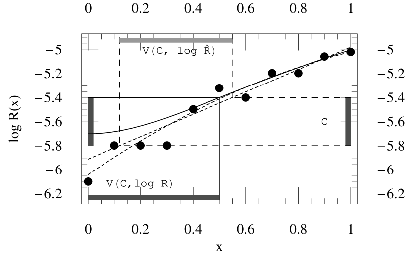
Figure 2.— Illustration of how small errors in fits can produce large uncertainties in the constraint-satisfying region, using a one-dimensional model. Solid line: the “true” function $\log R(x)=\log\mu(x)s/T$ [Eq. (8)], expressing the log of the average number of events expected for any $x$. Points: results of “experiments” for eleven values of the parameter $x$. Dotted lines: linear and quadratic least-squares fits to the data. Dark shaded boxes: (y-axis) the “constraint” interval $C=[-5.8,-5.4]$; (x-axis) the range of $x$ which truly satisfies the constraints [i.e., all $x$ so $\log R(x)\in C$; this region is denoted $V(C,\log R)$ in the notation of this paper]. Light shaded box: the interval predicted to satisfy the constraints, based on a linear fit [denoted $V(C,\log\hat{R}_{1})$ in the notation of this paper].

To increase the fraction of constraint-satisfying points included in a prediction – in the notation of this paper, to find a volume $V$ which contains the “naive” prediction $V(C,\log\hat{R}_{q})\subset V$ but contains more of the truly constraint-satisfying points $V(C,\log R)$ – the simplest option is simply to increase the size of the “constraint” interval. A larger constraint interval $C^{*}$ containing the original would automatically include more points in its predicted region (now $V(C^{*},\log\hat{R})$). While this prediction loses some of its reliability (i.e., we cannot ensure that only constraint-satisfying points lie in this region), we increase its robustness: by a good choice of $C^{*}$ we can almost guarantee that all constraint-satisfying points are included. Specifically, if we change the interval $C=\{c_{\rm min},c_{\rm max}\}$ to the broader interval $C^{*}(I)=\{c_{\rm min}-I,c_{\rm max}+I\}$ – that is, if we increase the constraint region by the size of the characteristic error in the fit – then any point $x$ which truly satisfies the constraints (in our notation, $x\in V(C,\log R)$) almost certainly lies within the larger “predicted” volume $V(C^{*},\log\hat{R})$. Formally, assuming the error at any point $|\delta\log R|$ is likely less than $I$, we conclude that $\log\hat{R}(x)=\delta\log R(x)+\log R(x)>\delta\log R(x)+c_{\rm min}\gtrsim-I+c_{\rm min}$ and similarly that $\log\hat{R}(x)\lesssim I+c_{\rm max}$. In the case shown in Figure 2, this error-widened prediction $V(C^{*}(I_{1}),\log\hat{R}_{1})$ includes both a higher fraction of constraint satisfying points ($r_{+}\simeq 92\%$) and a higher fraction of points which are not constraint satisfying ($20\%$).

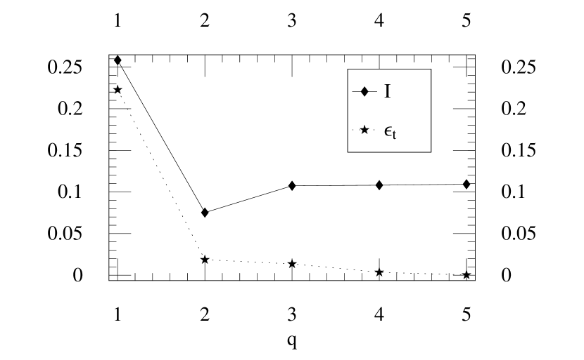
Figure 3.— Illustration of the balance between truncation and sampling error in a one-dimensional fit.

All these calculations, however, depend on the fit order: higher fit orders $q$ often allow more degrees of freedom with which to reproduce the true function $\log R(x)$ and therefore estimate $V(C,\log R)$. For example, assuming arbitrarily small (constant) errors and arbitrarily dense sampling $\vec{x}_{\alpha}$, the best possible $q$-th order polynomial least-squares fit is the orthogonal projection $P_{q}\log R$ of $\log R$ onto the space of $q$-th order polynomials, given in one dimension by

$$(P_{q}\log R)(x) = \sum_{l=0}^{q}\phi_{l}(x)\int_{0}^{1}dy\phi_{l}(y)\log R(y)$$

for $\phi_{l}(x)$ any set of orthonormal basis polynomials of degree $\leq l$ (e.g., $\phi_{l}(x)=\sqrt{2l+1}P_{l}(2x-1)$ where $P_{l}(x)$ are Legendre polynomials). Therefore, the minimum possible error of a $q$th-order polynomial fit is the magnitude $||P_{\perp q}\log R||$ of the difference $P_{\perp q}\log R\equiv\log R-P_{q}\log R$ between $\log R$ and this best fit, where $||f||^{2}=\int_{0}^{1}dx|f(x)|^{2}$. As the fit order increases, this “truncation error”

$$\epsilon_{t,q}\equiv||P_{\perp q}\log R||$$ (16)

decreases dramatically, as shown in Figure 3. However, the total error $I_{q}$ in the fit reflects a balance between (i) decreasing the “truncation error” with more degrees of freeom and (ii) increasing the “sampling error” as fewer data points are available per degree of freedom. For this reason, an optimal fit order exists, which provides the smallest error in $R(x)$, indicated by a minimum in $I_{q}$. This best fit order will provide the most reliable estimate of $V(C,\log R)$.

In principle, this one dimensional example contains all the core concepts we will apply to fitting seven-dimensional population synthesis results: the sampling uncertainty in each sample $n_{\alpha}$ of “simulated merger events”; the fit and its inaccuracies; the need to increase the size of the constraint interval and thus the “predicted” constraint-satisfying region to include a larger fraction of constraint-satisfying events; and a specific procedure for doing so, based on the characteristic errors of the fit. In practice, however, we must substantially flesh out this outline in two ways: (i) we must add a reliable way for estimating the fit error and selecting the optimal fit order without using $I$, since its definition in Eq. (14) uses the fit itself and requires exact, a priori knowledge of $R(x)$ (the function being fitted) that is not available in practice; (ii) we must extend the concepts developed here to seven dimensions, given the dependence of our population simulations.

3.2. Seven-Dimensional Analog

By virtue of existing in seven dimensions, the full population synthesis fitting problem is qualitatively different than the one-dimensional problem even with the same number of points and characteristic error. In the one-dimensional case, the many densely packed and relatively accurate samples of $R$ permit very accurate fits to $\log R$; barring rapid variation in $\log R$ with $x$, one-dimensional fits can easily have accuracies considerably exceeding the limiting accuracy of any individual measurement. On the other hand, in seven dimensions the same number of data points are much more loosely spaced (geometrically, the characteristic spacing is proportional to $N^{-1/d}$) and must constrain many more degrees of freedom at the same polynomial order, yielding much less accurate fits. For this reason, rather than attempt to rescale the number and uncertainties of our population synthesis simulations to generate a tractable one-dimensional analog, we instead demonstrate convergence using a seven-dimensional model that best captures the relevant features of our population synthesis data.

Explicitly, in this seven-dimensional toy model (i) the logarithm of the simulation size $\log N$ is gaussian distributed around $-4.5$ with an order of magnitude standard deviation, omitting simulations smaller than $10^{3}$ and larger than $10^{7}$; (ii) each set of simulation parameters $\vec{x}_{\alpha}$ is chosen by uniformly selecting seven random numbers $0\leq x^{k=1\ldots 7}_{\alpha}\leq 1$; (iii) the number of mergers $n_{\alpha}$ observed in any particular simulation parameterized by the seven parameters $\vec{x}_{\alpha}$ is drawn from a Poisson distribution with mean $\mu(\vec{x}_{\alpha})=\rho(\vec{x}_{\alpha})N$, where the mean number of mergers per binary $\rho(x)$ is defined by

$$\rho(\vec{x})=\mu(\vec{x})/N = 10^{-4x\cdot x/7-2.5}\;,$$ (17)

and thus (iv) implies a merger rate

$$R(\vec{x}) = \rho(\vec{x})(0.04{\rm yr}^{-1})$$ (18)

(again assuming $f_{b}=1$ and $\left<m_{2}\right>/\left<m_{1}\right>=0.5$). More specifically still, to compare with the array of $O(2000)$ simulations of merging NS-NS binaries, we generate a “model archive” of $N_{s}=2000$ randomly realized analogs, each defined by their parameter choices $\vec{x}_{\alpha}$, specific simulation sizes $N_{\alpha}$, observed merger numbers $n_{\alpha}$, and merger rates $\tilde{R}_{\alpha}=0.04{\rm yr}^{-1}(n_{\alpha}/N_{\alpha})$.

This seven-dimensional model qualitatively reproduces the distribution of merging double neutron star [NS-NS(m)] simulations in $(n,N)$ and $R$ [Fig. 4]. Quantitatively, this toy model is on average as accurate as our population synthesis simulations: the root-mean-square relative sampling error $\sigma_{E}$ (the “expected” standard deviation in the data, given the limiting error produced by sampling at each point)

$$\sigma^{2}_{E} \equiv \frac{1}{N_{s}}\sum_{\alpha=1}^{N_{s}}\left[n_{\alpha}(\ln 10)^{2}\right]^{-1}$$ (19)

of our population synthesis simulations $\sigma_{E}=0.25$ [see Table 2] agrees with the corresponding value $\sigma_{E}=0.24$ [see Table 1] for this seven-dimensional analog. Furthermore, in both cases this average accuracy $\sigma_{E}$ is still slightly smaller than the range in $\log R$, as characterized by $\sigma_{DD}$ (the “data-data” standard deviation, measuring the range of the distribution):

$$\sigma_{DD}^{2} = \frac{1}{N_{s}}\sum_{\alpha}\left[(\log\tilde{R}_{\alpha})^{2}-\left<\log\tilde{R}\right>^{2}\right]$$ (20)

($\sigma_{DD}=0.73$ for real simulations; $\sigma_{DD}=0.42$ for our toy model) Finally, as can be seen by comparing $N_{s}$, the number of population synthesis simulations, to $N_{s}^{+}$, the number of simulations with at least one event [Table 1], a significant fraction $O(10\%-50\%)$ of population synthesis simulations are totally unresolved; our seven-dimensional toy model has a similar fraction ($20\%$) of unresolved simulations.

Figure 4.— Comparison between our toy model (left) and simulations of merging NS-NS binaries (right). Top panels: scatter plot of the simulation size $N$ versus the number of merger events $n$ seen. Bottom panels: distribution of merger rates seen in simulation. In the right panels, no corrections are being made for the highly irregular patterns in which $N$ and $n$ were chosen, and which introduces unavoidable biases in the distribution of $\log(R)$.

3.3. Error Estimates and Convergence

Using this concrete and highly realistic seven-dimensional model problem described in §3.2, we can not only conclusively demonstrate that fairly accurate fits are possible for population syntheses, but we can also find a reliable estimate of the rms error in the fit, an estimate that can be reliably applied to surround all constraint-satisfying points inside a “predicted” volume. Precisely as in the one-dimensional case, given a fixed archive of seven-dimensional simulations, we can estimate $\log R$ with $\log\hat{R}_{q}$, the unique polynomial of order $\leq q$ that minimizes $\chi^{2}_{q}$, using any integer $q$ [Table 1]. With more degrees of freedom, higher-order fits can much more easily reproduce the data, so their mean square difference from the data $\sigma_{DF}$

$$\sigma_{DF}^{2} \equiv \frac{1}{N_{s}}\sum_{\alpha}\left[\log\hat{R}(\vec{x}_{\alpha})-\log\tilde{R}_{\alpha}\right]^{2}$$ (21)

(a “data-fit” comparison) decreases monotonically; see the fourth column of Table 1. But as these high order polynomials increasingly fit every sampling-induced flucuation in the data, high-order fits increasingly deviate from the exact solution: the exact rms error $I_{q}$ is also shown in Table 1 [calculated by comparing the fit to the known seven-dimensional model $R(x)$ from Eqs. (LABEL:eq:7d:R,eq:7d:mu)], showing $I_{q}$ has a minimum near an optimal fit order. Near this optimal fit order, the characteristic fit error $I_{q}$ is substantially less than the characteristic range of the data ($\sigma_{DD}$) – in fact, even less than the average statistical error of the sample $\sigma_{E}$. In other words, though this fit is accurate to only $20\%-30\%$ at any point (based on $10^{I_{q}}-1$ for $q=1\ldots 4$), this accuracy is sufficient to apply constraints, given the many orders of magnitude range spanned by $R(x)$.

Table 1Behavior of Sample Fit as Order Increases

$q$	$\chi^{2}$	$J$	$I$	$\sigma_{DF}$	$\sigma_{DD}$	$\sigma_{E}$
0	60.7	0.	0.462	0.421	0.421	0.241
1	4.16	0.373	0.138	0.228	0.421	0.241
2	1.3	0.104	0.0813	0.203	0.421	0.241
3	1.61	0.0475	0.0929	0.198	0.421	0.241
4	2.4	0.105	0.143	0.182	0.421	0.241

But while accurate fits exist, the tools presented henceforth provide few ways to identify them and particularly estimate their error without resorting to knowledge of the function being fit. For example, as we increase the available number of degrees of freedom, the root-mean-square difference $\sigma_{DF}$ between the fit and the data decreases monotonically to zero. Even at or near the optimal fit order, in our experience both $\sigma_{DF}$ and $\sigma_{E}$, the expected sampling-induced root-mean-square difference between data and predictions [Eq. (19)], correlate only weakly with the true error in the fit ($I_{q}$). A good fit can be identified using the weighted squared difference $\chi^{2}_{q}$, which does have a minimum value for a good fit. However, to understand and estimate the fit-induced error we must compare fits of successive orders with

$$J_{q} \equiv \left[\int d^{7}x\left[\log(\hat{R}_{q}/\hat{R}_{q-1})\right]^{2}\right]^{1/2}$$ (22)

This comparison between fits of different orders arises naturally from understanding how the error in the fit $I_{q}$ reflects a balance between (i) an increasing ability to fit $\log R$ exactly with more basis polynomials and ever smaller “truncation error”, decreasing the magnitude $||P_{\perp q}\log R||$ for $P_{\perp q}$ the and (ii) a decreasing statistical accuracy with fewer independent degrees of freedom $N_{s}-N_{\leq q}$ available to constrain the $N_{\leq q}$ independent coefficients in the expansion. These two terms contribute independently to the error at any fit order, allowing us to estimate $I_{q}$ by an incoherent superposition of “truncation error” and statistical error without explicitly calculating the best fit $\log\hat{R}_{q}$ itself:

$$I_{q}^{2} \simeq ||P_{\perp q}\log R||^{2}+\sigma_{E}^{2}\frac{N_{\leq q}}{N_{s}-N_{\leq q}}$$ (23)

with

$$N_{\leq q} \equiv \frac{(d+q)!}{d!q!}$$ (24)

Here $d=7$ is the dimension in which our functions are defined and $P_{\perp q}$ projects functions perpendicular to the space of basis polynomials of order less than or equal to $q$ [cf. Eq. (3.1)]: for example, if $\log R$ is a polynomial, $P_{\perp q}$ selects those coefficients of $\log R$ of order less than q. In this and other cases, this expression very accurately reproduces $I_{q}$; see for example Table 1.

When sampling errors are relatively small (i.e., $n_{\alpha}\gg 1$, so $\sigma_{E}\sim 0$), each successive approximation order $\log\hat{R}_{q}\simeq P_{q}\log R$ is found by orthogonal projection of $\log R$; therefore, for low fit orders the truncation error is just the magnitude of the next-highest-order correction to be applied, $J_{q}$:

$$||P_{\perp q}\log R||\simeq||\log\hat{R}_{q+1}-\log\hat{R}_{q}||\equiv J_{q+1}$$

In other words, for low $q$ we expect $I_{q}\simeq J_{q+1}$, as confirmed in Table 1.

From our experience with this and other model problems, the true rms fit error ($I_{q}$) is quite generally close to the change in the fit to the next order ($J_{q+1}$) and from the previous order ($J_{q}$). In particular, the difference between the current and next-lowest-order fit ($J_{q}$) has a minimum similar in magnitude and location to the minimum of $I_{q}$; see for example Table 1. We therefore use the order at which $J_{q}$ is smallest to select the optimal fit order and its value as the characteristic root-mean-square error in the fit.

3.4. Volume estimation

This error estimate provides the key tool needed to reliably and algorithmically surround almost all of the points with merger rates $R$ consistent with constraints, using information only about the fit, to the high level of accuracy needed to trust the results of multiple constraints. For example, observations of Galactic binary pulsars suggest double neutron star binaries merge in the Milky Way merge at a rate between $c_{\rm min}=\log(3\times 10^{-5}{\rm yr}^{-1})$ and $c_{\rm max}=\log(23\times 10^{-5}{\rm yr}^{-1})$. This constraint range turns out to lie on the high end tail of what our model simulations produce (Kim et al., 2003; O’Shaughnessy et al., 2007b). If our seven-dimensional model exactly described double neutron star merger rates, then only a small fraction of model parameters $\vec{x}\in V(C,\log R)$ ($5\%$ by volume of the unit seven-dimensional cube, corresponding to $|\vec{x}|<1.04$) reproduce observations. However, even though these merger rates correspond to the largest possible and therefore best-sampled predictions from population synthesis, the fit remains sufficiently inaccurate so that only $1-r_{+}\simeq 18\%$ of all constraint-satisfying points would not be included in a prediction $V(C,\log{\hat{R}})$ based on the fit alone. But based on Table 1, we can estimate the characteristic error in our fit by $J\simeq 0.05$. Therefore, when we compensate for this uncertainty with a wider constraint interval $C^{*}\equiv C^{*}(J)$, we much more accurately bound the set of constraint-satisfying points: $1-r_{+}(C^{*},\log\hat{R})=5\%$.

Strictly, the fraction of constraint-satisfying points that will be encompassed with a larger constraint interval $\tilde{C}$ depends strongly on the width and placement of the original interval $C$ – intuitively, an extremely narrow constraint requires extremely high-precision reconstruction of $R(\vec{x})$, in turn possible only at high merger rates $R$, where many events should be seen in simulation. However, the case shown here, with a very tight constraint (with only $5\%$ by volume of parameters satisfying the constraint), is substantially more difficult to satisfy than most individual observational constraints that can be applied in practice. Comparing our experience with model problems to the weak constraints available, we are confident that fewer than $5\%$ of constraint-satisfying systems will be omitted from $V(\tilde{C},\log\hat{R})$ when these volumes are constructed on the basis of real population synthesis simulations and corresponding observations. [The results of our broader array of model problems are available online in O’Shaughnessy et al. (2007a).]

4. Fitting: Population Synthesis Predictions

Almost exactly the same fitting techniques presented above are applied to our population synthesis data: we perform a weighted least-squares fit of polynomial-like basis functions over our seven-dimensional space, for each of the event rates of interest [BHBH(m), BHNS(m), NSNS(m), NSNS(vw), WDNS(e), WDNS(m), SNIb/c, and SNII, as introduced in §2.3]. For each fit, we evaluate the fit quality of several different polynomial orders to our data. To minimize the possibility of using more parameters than allowed by the number of our data points, we choose as “best” fit that order which minimizes the relative difference between fit orders $J_{q}$ (see below). However, we know that the merger rate $R(x)$ must satisfy certain symmetries, based on the manner in which we represent the kick velocity dispersion as a sum of two maxwellians (i.e., we can switch labels associated with the two distributions); therefore we limit the manner in which those parameters associated with kicks can enter into the distribution (see the Appendix).

Table 2Statistics of population synthesis simulations for event rates

Type	$N_{s}$	$N_{s,+}$	$\bar{N}_{\leq q}$	$q$	$\chi^{2}$	$\sigma_{DF}$	$J_{q}$	$\sigma_{E}$	$\sigma_{DD}$	$\eta(10)$
BH-BH(m)	2930	1201	141	3	15.5	0.77	0.67	0.25	0.78	12%
BH-NS(m)	2533	1334	141	3	11.1	0.53	0.40	0.23	0.71	2%
NS-NS(m)	2803	2382	141	3	18.4	0.37	0.22	0.14	0.63	5%
NS-NS(vw)	1325	1087	141	3	16.7	0.39	0.37	0.13	0.76	8%
WD-NS(e)	1770	1564	141	3	12.5	0.34	0.20	0.14	0.57	10%
WD-NS(m)	1770	1658	141	3	16.4	0.34	0.19	0.13	0.45	11%
SN Ib/c	1482	1482	141	3	7.8	0.07	0.06	0.02	0.11	n/a
SN II	1482	1482	141	3	6.0	0.04	0.02	0.03	0.17	n/a

Table 2 summarizes the properties of the least-squares fits we applied to our archived population synthesis results. The first column provides a brief label for the fit, as described in greater detail in the text. The next two columns summarize the amount of available information contained in our population synthesis archive: $N$ is the number of population synthesis models with unbiased data (i.e., where all plausible progenitors for the target event have been included), whereas $N_{+}$ is a smaller number of models with unbiased data containing one or more events (i.e., for which an estimate of the rate, rather than merely an upper bound, is possible). The next block of five columns describes properties and diagnostics of a weighted least-squares fit applied to our data. The first two columns, $q$ and $\bar{N}_{\leq q}$, merely indicate the polynomial order and number of degrees of freedom involved in our fit ($\bar{N}_{\leq q}$ differs from $N_{\leq q}$ introduced earlier due to the symmetry requirement described above). In all the cases shown here, the optimal polynomial order produces far fewer degrees of freedom than population synthesis simulations (i.e., $\bar{N}_{\leq q}\ll N_{s,+}$).

The next three columns provide critical diagnostics of our fit: $\chi^{2}$, $\sigma_{DF}$, and $J_{q}$ [Eqs. (11,19,22)]. All three columns roughly measure our “goodness-of-fit”; based on our experience with model problems and our understanding of the values these quantities should take for fits dominated by statistical and truncation errors, all three universally indicate that truncation error dominates – that is, that our low-order polynomial basis functions are not sufficiently general models to match the exact merger rate $R(x)$ implied by our population synthesis simulations. For example, the limiting value of $J_{q}$ is significantly above the level of sampling error $\sigma_{E}/\sqrt{N_{s,+}/\bar{N}_{\leq q}}$ suggested by the second term in Eq. (23) – that is, above the level of error expected when averaging $N_{s,+}/N_{\leq q}$ simulation samples per degree of freedom, each with characteristic error $\sim\sigma_{E}$. This high level of error suggests fit accuracy is limited by truncation error – inability to fit the exact form of $R(x)$ with our basis polynomials – rather than sampling uncertainties at each point. Additionally, as illustrated in our discussion of seven-dimensional model problems, the latter two columns provide the logarithmic uncertainty in our fits; for example, fits with $J\simeq 0.33$ are known to within a factor two with one-sigma confidence. These columns should be contrasted with the next two, which provide the average sampling-induced uncertainty $\sigma_{E}$ in the data [Eq. (19)] and the characteristic range of merger rates $\sigma_{DD}$ seen in simulation [Eq. (20)]. Our fits remain useful so long as their uncertainties are much less than the range of $\log R$ (i.e., so long as $J\lesssim\sigma_{DD}$). As seen in Table 2, our best fit satisfies this requirement ($J\lesssim\sigma_{DD}$) for each populations of interest.

The last column provides the fraction $\eta$ of simulations with no events when more than $10$ would be expected based on the fit. Based on an average uncertainty of a characteristic factor of two in the fit (our best fits have $J\simeq 0.33$, corresponding to a merger rate known to within a factor $2\simeq 10^{J}$), we would estimate that the fraction of simulations $\eta$ which produce no merger events when more than 10 should be seen based on our uncertain estimate of the event rate should be comparable to or smaller than the fraction of simulations which should produce $10/2=5$ events but in fact produce zero, namely $\eta\lesssim p(0,10/2)\simeq 0.7\%$ [Eq. (6)]. However, regions with the lowest merger rates will be undersampled and therefore have characteristic uncertainties marginally larger (e.g., up to a factor $3$ to $4$), leading to $\eta$ of a few to ten percent.

4.1. Results

Supenovae: Given our choice of stellar mass interval probed in our simulation (i.e., $m_{1}>4M_{\odot}$), supernovae occur extremely frequently, providing us with superb statistics at low cost. However, our limited set of basis functions can only with difficulty reproduce the observed variation in supernovae rates: even though SN rates for models in our archive are at times known to $1\%$ (i.e., involving $10^{4}$ or more sampled events), or $0.004$ in the log, our optimal fit differs significantly from the data, by $\sigma\simeq O(0.04)$ in the log.

Nonetheless, as discussed in the forthcoming O’Shaughnessy et al. (2007b), the supernovae rate remains a striking success of the StarTrack population synthesis code and our normalization conventions (e.g., $\dot{M}\simeq 3.5M_{\odot}{\rm yr}^{-1}$). No matter what combination of population synthesis parameters we choose, the predicted SN rates lie well within the observational constraints found by Cappellaro et al. (1999).

WD-NS binaries: As with supernovae, white dwarf-neutron star binaries occur fairly frequently,allowing us to accumulate fairly good statistics over a broad range of population synthesis parameters. Additionally, based on the distribution of $N_{s}$ versus $n$ (i.e., as in Figure 5), our sample shows no signs of systematic incompleteness: we appear to have covered the full range. Though our polynomial fits continue to introduce systematic error, the resulting fit behaves well throughout the range.

BH-BH binaries: Double black hole binaries, in contrast, occur extremely infrequently, especially with an assumed maximum NS mass of $2.5M_{\odot}$, instead of $2.0M_{\odot}$, as assumed in O’Shaughnessy et al. (2005a, b). [The inefficient formation of coalescing BH-BH binaries is discussed and explained in more detail by Belczynski et al. (2006b).] Nonetheless, by using special-purpose partitions, O’Shaughnessy et al. (2005a) accumulated a large ($\simeq 500$ simulations) sample with good ($n\simeq 10$) statistics on a large subset of parameter space; though these simulations assumed a maximum NS mass of $2M_{\odot}$, we post facto changed the maximum NS mass to $2.5M_{\odot}$. By adjoining the results of general-purpose simulations not assured of good statistics, this sample has since been enlarged by a factor $\simeq 5$, with emphasis on the same subset of parameter space presented in O’Shaughnessy et al. (2005a) (see Figure 1). Finally, though the distribution of $n$ versus $N_{s}$ (Figure 5) suggests the lowest BH-BH merger rates may not be very well-resolved, we have no reason to suspect we have any significant under-resolved region: simulations larger than $10^{6}$ binaries consistently produce several merger events ($n\gg 0$).

Nonetheless, the BHBH(m) fit is comparatively poor: even though the average simulation with binary black holes produces enough to fairly accurately determine the rate (i.e., $\sigma_{E}\simeq 0.25$), our best fit is barely more accurate than approximating the average BH-BH merger rate seen in simulations (i.e., compare the characteristic fit error $J_{q}\simeq 0.67$ with the range of BH-BH merger rates seen in simulation, $\sigma_{DD}\simeq 0.78$).

Results: NS-NS and BH-NS binaries: Despite (or perhaps because of) a concerted effort to accumulate good statistics targeted specifically to these classes, fits for NS-NS and BH-NS event rates are statisticallly implausible as measured by $\chi^{2}$. Judging from Figure 5, the NSNS(m) and BH-NS(m) are comparatively well-resolved: longer simulations fairly consistently have a lower chance of producing $n=0$ results. For this reason, we strongly suspect some feature of these underlying rate functions are poorly-described by our basis functions; we intend to more thoroughly test this hypothesis (with better statistics) by comparing these fits to nonparametric estimates in a future paper.

5. Conclusions

To develop a more comprehensive understanding of population synthesis predictions and to allow those theoretical predictions to be systematically compared with observations of the end products of high-mass single and binary stellar evolution, we have fit eight predictions from the StarTrack code over seven of its input parameters. These fits are available on requests sent to the first author. In a companion paper, O’Shaughnessy et al. (2007b) apply these fits along with estimates of their systematic errors to discover robust constraints on the seven parameters that enter into population synthesis. Additionally, we have demonstrated that in analagous model problems the constraint-satisfying region defined by using these fits can, under appropriate conditions, very accurately trace the underlying constraint-satisfying region. Finally, we have presented a thorough diagnostic formalism, including a large list of diagnostic quantities and tests ($I,J,\sigma_{E,DF,DD},\chi^{2},\eta,r_{+}$, etc.), which can be applied to studies of fits to large archives of any (individual) population synthesis code.

Appendix A Sampling, prior distributions and the likelihood of results

In Figure 6 we compare the distribution of merger rates derived directly from our current database of simulations (dotted lines) to the distribution of merger rates derived from the corresponding fit (solid lines) obtained using the methodology described here. Unlike Figure 3 of O’Shaughnessy et al. (2005b), in which the simulations being fit had parameters drawn randomly from the entire range of parameters allowed, in this study the simulations were not randomly distributed through the entire parameter range; see for example Figure 1. In effect, the rate distributions drawn from simulations and fits assume significantly different priors for population synthesis model parameters, the former favoring lower kicks. Therefore, although the distributions appear different in shape, they reflect the same physical process, just with different priors regarding what model parameters are likely. In particular, the fitted rate results represent the unbiased distributions of rates with uniform coverage of the seven-dimensional model parameter space. Furthermore these distributions fully account for uncertainties in the fits, as described in §4.

To phrase the same statement more abstractly, our prior expectations about the relative likelihood of population synthesis parameters (e.g., kicks) influences our expectations for the relative likelihood of different merger rates. If at any point our knowledge of binary properties, evolution, and compact object kicks improves to a degree such that we can confidently move away from flat priors into favoring certain, more specific priors for the model parameters, then the shape of the probability distributions derived from fits will change accordingly, expressing the influence of the adopted priors.

Figure 5.— Log-log scatter plot of the number of events seen in a sample against the population synthesis sample size. Also shown is a diagonal line corresponding to the 99% lower bound on the fit-predicted rate distribution, translated from physical rate into expected number of events seen per unit population synthesis sample size. For completeness, models with zero events are shown with $\log_{10}n$ as $-1$.

Figure 6.— Probability distributions for formation rates for different types of binaries in the Milky Way. Dotted lines: the distributions of rates derived directly from our database of simulations, which does not regularly sample the model parameter space; cf. Figure 1. Thin solid curves: the distribution of different formation rates derived using fits, using precisely the same sampling as the raw data (dotted line). Heavy solid curve: the distributions derived from our fits to the simulations when the model parameter space is sampled uniformly. In all cases, the formation rate data is smoothed with a gaussian of standard deviation $0.1$. It is evident that: (i) the quality of the fits is rather good; and (ii) the change in the shape of the distributions is primarily because of the different priors between the dotted and thick-solid lines. Last we note that: (i) the rate results for binaries involving BHs are most uncertain because of the assumed maximum NS mass of $2.5M_{\odot}$ that reduces the overall formation rates for BH binaries (compared to an assumed maximum mass of $2M_{\odot}$); (ii) all rates quoted in this studies are for Milky-Way like galaxies and we do not account for any differences associated with elliptical galaxies.

Appendix B Polynomial basis functions

To parameterize supernovae kick distributions, StarTrack employs three parameters, $\sigma_{1}$, $\sigma_{2}$, and $s$, which represent the superposition of two Maxwellian kick distributions with probabilities $s$ and $1-s$. The physical predictions associated with $(\sigma_{1},\sigma_{2},s)$ are therefore identical to those of $(\sigma_{2},\sigma_{1},1-s)$. To improve the physical significance of our fit, we have chosen to employ basis polynomials which enforce this requirement to all orders.

Specifically, rather than allow for homogeneous basis polynomials in these parameters, we use the following, for arbitrary $p$ and $q$:

$$\sigma_{1}^{p}s^{q}+\sigma_{2}^{p}(1-s)^{q}$$ (B1)

$$2\sigma_{1}^{p}\sigma_{2}^{p}s(1-s)+\sigma_{1}^{2p}s^{2}+\sigma_{2}^{2p}(1-s)^{2}$$ (B2)

Because $s$ must enters in a heterogeneous manner to preserve our desired symmetry, these basis polynomials are of a fixed order in all kick parameters. For the purposes of order counting when constructing fits, the first polynomial is denoted order $p+q$ and the second order $p$.

References

- Abbott et al. (2005a) Abbott, B., Abbott, R., Adhikari, R., Ageev, A., Allen, B., Amin, R., Anderson, S. B., Anderson, W. G., Araya, M., Armandula, H., Ashley, M., Asiri, F., Aufmuth, P., Aulbert, C., Babak, S., Balasubramanian, R., & OTHERS. 2005a, Phys. Rev. D, 72, 082002 [ADS] [ADS]
- Abbott et al. (2005b) Abbott, B., Abbott, R., Adhikari, R., Ageev, A., Allen, B., Amin, R., Anderson, S. B., Anderson, W. G., Araya, M., Armandula, H., Asiri, F., Aufmuth, P., Aulbert, C., Babak, S., Balasubramanian, R., Ballmer, S., Barish, B. C., Barker, D., Barker-Patton, C., & OTHERS. 2005b, Phys. Rev. D, 72, 082002
- Arzoumanian et al. (1999) Arzoumanian, Z., Cordes, J. M., & Wasserman, I. 1999, ApJ, 520, 696 [ADS]
- Belczynski et al. (2002) Belczynski, K., Kalogera, V., & Bulik, T. 2002, ApJ, 572, 407 [ADS]
- Belczynski et al. (2006a) Belczynski, K., Kalogera, V., Rasio, F., Taam, R., Zezas, A., Maccarone, T., & Ivanova, N. 2006a, arxiv eprint [URL]
- Belczynski et al. (2006b) Belczynski, K., Taam, R. E., Kalogera, V., Rasio, F. A., & Bulik, T. 2006b, ApJ. (accepted); eprint astro-p0h/0612032 [ADS]
- Cappellaro et al. (1999) Cappellaro, E., Evans, R., & Turatto, M. 1999, A&A, 351, 459 [ADS]
- Fryer et al. (1998) Fryer, C., Burrows, A., & Benz, W. 1998, ApJ, 496, 333 [ADS]
- Hobbs et al. (2005) Hobbs, G., Lorimer, D. R., Lyne, A. G., & Kramer, M. 2005, MNRAS, 360, 974 [ADS]
- Hurley et al. (2002) Hurley, J. R., Tout, C. A., & Pols, O. R. 2002, MNRAS, 329, 897 [ADS]
- Kalogera et al. (2005) Kalogera, V., Kim, C., Lorimer, D. R., Ihm, M., & Belczynski, K. 2005, in ASP Conf. Ser. 328: Binary Radio Pulsars, ed. I. Stairs, 261–+
- Kim et al. (2003) Kim, C., Kalogera, V., & Lorimer, D. R. 2003, ApJ, 584, 985 [ADS]
- Kim et al. (2004) Kim, C., Kalogera, V., Lorimer, D. R., & White, T. 2004, ApJ, 616, 1109 [ADS]
- Lacey & Fall (1985) Lacey, C. G. & Fall, S. M. 1985, Astrophysical Journal, 290, 154
- Lorimer (2005) Lorimer, D. 2005, Living Reviews in Relativity, 2005-7 [URL]
- Nice et al. (2005) Nice, D. J., Splaver, E. M., Stairs, I. H., Löhmer, O., Jessner, A., Kramer, M., & Cordes, J. M. 2005, ApJ, 634, 1242 [ADS]
- O’Shaughnessy et al. (2005a) O’Shaughnessy, R., Kalogera, V., & Belczynski, K. 2005a, ApJ, 620, 385 [ADS]
- O’Shaughnessy et al. (2007a) —. 2007a, Submitted to ApJ (astro-ph/0609465) [URL]
- O’Shaughnessy et al. (2005b) O’Shaughnessy, R., Kim, C., Fragos, T., Kalogera, V., & Belczynski, K. 2005b, ApJ, 633, 1076 [ADS] [ADS]
- O’Shaughnessy et al. (2007b) O’Shaughnessy, R., Kim, C., Kalogera, V., & Belczynski, K. 2007b, Submitted to ApJ (astro-ph/0610076) [URL]
- Portegies Zwart & Verbunt (1996) Portegies Zwart, S. F. & Verbunt, F. 1996, A&A, 309, 179 [ADS]
- Rana (1991) Rana. 1991, Annual reviews of astronomy and astrophysics, 29, 129 [URL]
- Splaver et al. (2002) Splaver, E. M., Nice, D. J., Arzoumanian, Z., Camilo, F., Lyne, A. G., & Stairs, I. H. 2002, ApJ, 581, 509 [ADS]