Giant Molecular Clouds in M31 – I: Molecular Cloud Properties

Abstract

We present Berkeley Illinois Maryland Association (BIMA) millimeter interferometer observations of giant molecular clouds (GMCs) along a spiral arm in M31. The observations consist of a survey using the compact configuration of the interferometer and follow-up, higher-resolution observations on a subset of the detections in the survey. The data are processed using an analysis algorithm designed to extract GMCs and correct their derived properties for observational biases thereby facilitating comparison with Milky Way data. The algorithm identifies 67 GMCs of which 19 have sufficient signal-to-noise to accurately measure their properties. The GMCs in this portion of M31 are indistinguishable from those found in the Milky Way, having a similar size-line width relationship and distribution of virial parameters, confirming the results of previous, smaller studies. The velocity gradients and angular momenta of the GMCs are comparable to the values measured in M33 and the Milky Way; and, in all cases, are below expected values based on the local galactic shear. The studied region of M31 has a similar interstellar radiation field, metallicity, Toomre $Q$ parameter, and midplane volume density as the inner Milky Way, so the similarity of GMC populations between the two systems is not surprising.

1. Introduction

As the instrumentation for millimeter-wave telescopes improves, it becomes progressively more straightforward to study individual molecular clouds in other galaxies. Recent studies of Local Group galaxies have surveyed large numbers of molecular clouds in the Large Magellanic Cloud (Mizuno et al., 2001b), the Small Magellanic Cloud (Mizuno et al., 2001a), M33 (Engargiola et al., 2003), and a bevy of Local Group dwarf galaxies (e.g.  Wilson, 1994; Taylor et al., 1999). These recent studies explore the nature of star formation on galactic scales by studying the properties of giant molecular clouds (GMCs, $M>10^{5}~{}M_{\odot}$) throughout their host galaxies. Such GMCs contain the majority of the molecular mass in the Milky Way’s ISM and are responsible for most of the star formation in the Galaxy (Blitz, 1993).

The Andromeda Galaxy (M31) is the second largest disk galaxy in the Local Group, after the Milky Way, and it subtends over 2 deg² on the sky. Its proximity (770 kpc, Freedman & Madore, 1990) makes it an excellent target for studying extragalactic molecular clouds. Numerous surveys of CO emission have been conducted over a portion of M31 and a comprehensive list of the 24 CO studies published up to 1999 is given in Loinard et al. (1999). This extensive list of surveys can be supplemented with a few major studies that have occurred since then. Sheth et al. (2000, 2006) used the BIMA millimeter interferometer to study a $3^{\prime}$ field in the outer region of the galaxy ($R_{gal}=12$ kpc) and find 6 molecular complexes similar to those found in the Milky Way. An extensive survey covering the entirety of the star-forming disk of M31 has been completed using the IRAM 30-m by Nieten et al. (2006, see also references therein). Finally, Muller (2003) used the Plateau de Burre interferometer to examine the properties of molecular clouds in 9 fields. Using the GAUSSCLUMPS (Stutzki & Güsten, 1990; Kramer et al., 1998) algorithm, they decompose the emission into 30 individual molecular clouds.

Previous high-resolution observations of CO in M31 indicate that a large fraction of the molecular gas is found in GMCs. Identifying individual GMCs requires a telescope beam with a projected size $\lesssim 50$ pc, the typical size of a GMC in the Milky Way (Blitz, 1993), which requires an angular resolution of $14^{\prime\prime}$ at the distance of M31. There have been seven observational campaigns that observed CO $(1\to 0)$ emission from M31 at sufficient resolution to distinguish molecular clouds: Ichikawa et al. (1985); Vogel et al. (1987); Lada et al. (1988); Wilson & Rudolph (1993); Loinard & Allen (1998); Sheth et al. (2000); Muller (2003). With the exception of Loinard & Allen (1998), all of these studies have found GMCs with properties similar to those found in the inner Milky Way and Melchior et al. (2000) have argued that the differences observed by Loinard & Allen (1998) can be attributed to observational errors. Indeed, Vogel et al. (1987) presented the first direct observations of GMCs in any external galaxy using interferometric observations. Subsequent studies with interferometers and single-dish telescopes confirmed that most CO emission in M31 comes from GMCs and that the GMCs properties were similar to those found in the Milky Way (Lada et al., 1988; Wilson & Rudolph, 1993; Sheth et al., 2000; Muller, 2003).

Although the molecular gas in M31 has been extensively studied, there remains a gap connecting the large-scale, single-dish observations and the small-scale, interferometer observations. To address this gap, we completed CO($J=1\to 0$) observations of a large (20 kpc² region) along a spiral arm of M31 with high resolution ($\sim 50$ pc). We then followed up on these observations using a more extended configuration of the interferometer yielding data with a resolution of $\sim 25$ pc. This paper presents the observational data of the both the survey and the follow-up observations (§2). Using only the follow-up data, we present the first results, namely a confirmation of previous studies that find GMCs in M31 are similar to those in the Milky Way (§§3,4). Notably, this paper utilizes the techniques described in (Rosolowsky & Leroy, 2006) to correct the observational biases that plague extragalactic CO observations, thereby placing derived cloud properties on a common scale that can be rigorously compared with GMC data from other galaxies. The follow-up observations are also used to examine the velocity gradients and angular momentum of the GMCs, which are then compared to the remainder of gas in the galaxy for insight into the GMC formation problem (§5). We conclude the paper by examining the larger galactic environment of M31 to explore connections between the GMCs and the larger ISM (§6). Subsequent work will explore the star formation properties of these GMCs and the formation of such clouds along the spiral arm using the data from the spiral arm survey.

2. Observations

We observed ¹²CO($J=1\to 0$) emission from M31 during the spring and fall observing seasons of 2002 with the D and C configurations of the BIMA millimeter interferometer (Welch et al., 1996). The observations consisted of an 81-field mosaic using the most compact (D) configuration with follow-up observations on seven sub-regions, covering 30 fields at higher resolution (C array). The D-array survey spans a projected length of 6.7 kpc along a spiral arm in the galaxy. Three of the seven follow-up, C-array fields targeted regions with known CO emission from the D-array survey, and the remaining four fields targeted regions with strong CO emission in the single-dish observations of Dame et al. (1993) over a range of galactocentric distances. The locations of the fields are indicated in Figure 1.

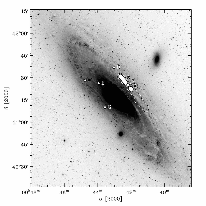
Figure 1.— The Digital Sky Survey image of M31 with the locations of the interferometer observations indicated. The extent of the D-array spiral arm survey is indicated with the black and white dashed contour. The targets of the C-array follow-up observations are indicated with white regions. Letters next to the C-array fields indicate the corresponding fields in Table 1.

The D-array observations were completed in September and October 2002 over the course of four nights. Each night roughly 20 pointings of the mosaic were observed. During the observations, the fields were observed for 46 seconds each, making two passes through the mosaic before returning to the phase calibrator (0102+504, 2.6 Jy) every 30 minutes. This cycle was continued through the night, accumulating $\sim 6$ hours of integration time on M31 per night (18 minutes per field). The correlator was configured to span 200 MHz at 500 kHz (1.3 km s^-1) resolution, easily encompassing the whole range of velocities expected from the M31’s rotation curve for this region (Ibata et al., 2005). At the latitude of the Hat Creek Radio Observatory, M31 transits near zenith and cannot be observed for 40 minutes a night. This time was used to perform flux calibrations using Saturn and Uranus. Over the course of the observations, the derived flux of the phase calibrator was stable to 10%. The relative flux calibration of the data may be better than this level owing to the intrinsic variability of the phase calibrator.

The data were reduced and inverted using the MIRIAD software package (Sault et al., 1995), following the calibration procedures of the BIMA Survey of Nearby Galaxies (Helfer et al., 2003). The four nights of $uv$ data were combined using a linear mosaicing technique. The inversion used natural weighting, and gridding in the $uv$ plane was chosen to produce maps with $3^{\prime\prime}$ pixels and $2.03$ km s^-1 channel width. The dirty maps were deconvolved with a Steer-Dewey-Ito deconvolution algorithm optimized for mosaics (MOSSDI2 in the MIRIAD software package). Each plane of the final image was cleaned to the 1.5$\sigma_{rms}$ significance level. The final resolution of the survey is $14^{\prime\prime}$, with negligible variation over the map. The mosaic is corrected for the gain of the primary beam.

Three regions within the D-array survey containing emission were observed with the more extended C-array configuration. In total, 26 fields were observed on five nights from October to December 2002. The C-array observations used the same observing strategy as the low-resolution survey, observing each field for 46 seconds and making two or three passes (depending on the size of the mosaic) through the mosaic before observing the phase calibrator every 24 minutes. The correlator configuration and choice of calibrators were the same as for the survey. The follow-up observations used a subset of the D-array pointing centers to facilitate merging the two data sets. These data were combined with the D-array observations in the $uv$ plane and inverted using uniform weighting. The data were cleaned using the same Steer-Dewey-Ito deconvolution algorithm as for the D-array map. The final resolution of the combined data is $\sim 9^{\prime\prime}$ with a 2.03 km s^-1 channel width. The images are corrected for the gain of the primary beam.

Prior to the D-array survey, four fields of M31 were observed using the C array (Spring 2002). These observations targeted single fields known to contain bright CO emission from Dame et al. (1993) over a range of galactocentric distance. The fields were chosen to span a variety of regions in the galaxy (different spiral arms and galactocentric radii) in an attempt to reveal any biases seen by focusing on one region of the galaxy. The observations used 0136+478 as a phase calibrator and Mars to establish the flux scale of the phase calibrator. Since the observations consisted exclusively of C-array data, they were inverted using natural weighting. The final synthesized beam size for these observations is $7.5^{\prime\prime}$.

The observations produced one survey data cube and 7 high-resolution data cubes for analysis. The properties of these data sets are summarized in Table 1. Since space constraints prohibit a full presentation of all the observational data, an excerpt from the center of Field A is shown in Figure 2 to illustrate typical quality of the data. The remainder of the paper emphasizes the high-resolution data (Fields A-G in Table 1). We defer presentation and analysis of the Survey data to a subsequent paper.

Table 1 Summary of BIMA observations of M31.

Field	Conf.	Center	Resolution	Size	Noise	$f_{rec}$
		($\alpha_{2000},\delta_{2000}$)	(${}^{\prime\prime}\times\mbox{km/s}$)	(${}^{\prime\prime}\times^{\prime\prime}\times\mbox{km/s}$)	(K km/s)
Survey	D	00 41 48.1, +41 19 02	$14\times 2.03$	$1885\times 350\times 215$	0.27	0.35
A	C,D	00 42 26.5, +41 28 45	$8.2\times 2.03$	$255\times 205\times 102$	0.64	0.35
B	C,D	00 42 12.3, +41 25 33	$10.3\times 2.03$	$570\times 320\times 102$	0.54	0.12
C	C,D	00 42 02.4, +41 22 13	$10.2\times 2.03$	$305\times 250\times 102$	0.76	0.17
D	C	00 43 01.8, +41 37 00	$7.0\times 2.03$	$100\times 100\times 100$	0.48	0.42
E	C	00 43 56.8, +41 26 12	$8.1\times 2.03$	$100\times 100\times 100$	0.94	0.23
F	C	00 44 44.3, +41 28 07	$7.2\times 2.03$	$100\times 100\times 100$	0.92	0.15
G	C	00 43 33.9, +41 09 58	$7.1\times 3.04$	$100\times 100\times 100$	1.38	0.19

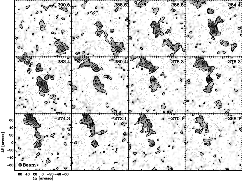
Figure 2.— Channel maps of an excerpt from the center of Field A. Only 12 channel maps containing significant CO emission are shown. The gray scale of the channel map runs linearly from 0 to 6 K km s^-1. Contours of local significance are shown at $-4,-2$ (gray),2, 4, 8, and 12 times the local value of $\sigma_{rms}$. At the center of the field, $\sigma_{rms}=0.4$ K km s^-1, though this value changes across the map owing to variable gain from the interferometer. Each channel map is annotated in the upper, right-hand corner with $V_{\mathrm{LSR}}$ for the channel in km s^-1. For reference, the center of the field is at $\alpha_{2000}=00^{\mathrm{h}}~{}42^{\mathrm{m}}~{}29\fs 3$, $\delta_{2000}=+41^{\circ}~{}28^{\prime}~{}53\farcs 3$ and the extent of the displayed region is indicated in Figure 3.

3. Analysis of the Molecular Emission

3.1. Signal Identification

For data cubes A–G in Table 1, we identified the emission using a dynamic thresholding technique. For every pixel in the cube, we first estimated the rms value for the noise using the method of Engargiola et al. (2003); this method accounts for gain variations in both position and frequency. We first estimate the noise at every position by measuring the standard deviation of the data values using iterative rejection of high signal pixels ($>3\sigma_{rms}$). We generate a noise map by smoothing the resulting pixel estimates with a boxcar kernel of the same size as the synthesized beam. Then, we estimate the relative changes of the noise across the bandpass by estimating $\sigma_{rms}$ in each channel map and normalizing to the mean value of $\sigma_{rms}(v)$ across the bandpass. We generate a cube of noise estimates by scaling the error map by the fractional change from the mean appropriate for that velocity. Performing a pixel-wise division of the data cube by the cube of noise estimates yields a data set in significance units.

We identify CO emission in the data cubes by searching for contiguous regions of high significance in position-position-velocity space using a two-tiered thresholding scheme (e.g.  Scoville et al., 1987). The core pixels in the mask are identified as pairs of pixels in adjacent velocity channels with $I(x,y,v)>4\sigma_{rms}(x,y,v)$. The mask is then expanded in position and velocity space to include all pixels with $I>2\sigma_{rms}$ that are connected by high significance pixels to the $4\sigma_{rms}$ core of the mask. This masking process has been used in previous extragalactic, interferometric studies and has been shown to successfully identify emission with minimal inclusion of noise (Engargiola et al., 2003). Eliminating noise from the emission under consideration is key to the methods used to determine cloud properties (see §3.3).

3.2. Inclination Effects

The identification and analysis of GMCs in M31 may be complicated by the relatively high inclination of the galaxy: $i=77^{\circ}$ (Walterbos & Kennicutt, 1988). The situation is similar, in part, to observing GMCs in the outer regions of the Milky Way ($i=90^{\circ}$!), and the spatial resolution ($\sim 25$ pc) is comparable to what is found using small telescopes (e.g. the CfA 1.2-m) to observe distant ($>10$ kpc) GMCs in the Milky Way (Dame et al., 2001). While study of GMCs has been conducted in the Milky Way with such data, the inclination being $77^{\circ}$ and not $90^{\circ}$ helps the situation significantly. The foreground and background spiral arms in M31 are separated from the arm under consideration by $>2^{\prime}$ in projection. Thus, spatial information is useful for separating the emission into GMCs. The clouds in the interarm region are likely too faint to be recovered by the deconvolution algorithm (§3.4). We conclude that the primary concern in decomposition is the blending of GMCs within the same spiral arm. Nieten et al. (2006) estimate that the width of the spiral arms in the plane of the galaxy for this region is $\sim 500$ pc with a vertical thickness of 150 pc. There could be multiple, distinct clouds in the spiral arm along the same line of sight, so we make a simple estimate of how many GMCs are likely to be along a line of sight through the spiral arm. We model the arm as a cylinder with elliptical cross-section having major and minor axes of 500 pc and 150 pc respectively. For a viewing angle 77^∘ away from the minor axis of the cylinder, the path length through the cylinder is $\ell=400$ pc. We assume that the GMCs are distributed uniformly in the cylindrical volume with volume density $n$ and geometric cross-section $\sigma$. The mean number of clouds intersected by a line-of-sight through the arm is then $n\sigma\ell$. We estimate $n$ by counting the number of clouds ($N$) in some trial volume along the arm $V=\pi LWH/4$ where $L$,$W$ and $H$ represent the length, width (major axis) and height (minor axis) of the volume of the arm respectively. By assuming a surface density through a typical GMC of $\Sigma_{GMC}$ and comparing this to the observed surface density in the single-dish map $\langle\Sigma_{\mathrm{H2}}\rangle$, we can estimate the area filling fraction of GMCs in the arm when viewed from above the galaxy:$f=\langle\Sigma_{\mathrm{H2}}\rangle/\Sigma_{GMC}$. Since $f$ is also given by $N\sigma/LW$, we can express

$$n\sigma\ell=\frac{4\ell\langle\Sigma_{\mathrm{H2}}\rangle}{\pi H\Sigma_{GMC}}.$$ (1)

Significant confusion will occur for $n\sigma\ell\gtrsim 1$. For this condition to be met with $\ell=400$ pc and $H=150$ pc, $\langle\Sigma_{\mathrm{H2}}\rangle/\Sigma_{GMC}>0.3$. The data of Nieten et al. (2006) show $\langle\Sigma_{\mathrm{H2}}\rangle\approx 5~{}M_{\odot}\mbox{ pc}^{-2}$ for this region requiring GMCs in M31 to have $\Sigma_{GMC}<20~{}M_{\odot}\mbox{ pc}^{-2}$ for significant blending to occur. We regard this possibility as unlikely since GMCs in other, less confused regions of M31 are found to have comparable properties to Local Group clouds (Sheth et al., 2000; Muller, 2003) where $\Sigma_{GMC}\approx 100~{}M_{\odot}\mbox{ pc}^{-2}$ (Solomon et al., 1987; Blitz et al., 2006). Unfortunately, one of the aims of the paper is to assess how similar clouds in M31 are to those in other galaxies; so we cannot reject the possibility that the clouds could be significantly blended along the line of sight although this would imply significantly larger sizes and lower column densities than is typical for GMCs in other galaxies.

We conclude this discussion of inclination effects by noting that we will assume that GMC properties are independent of viewing angle, as is common in studies of GMCs in the Milky Way and beyond (e.g. Scoville et al., 1987; Solomon et al., 1987; Wilson & Scoville, 1990; Wilson & Rudolph, 1993; Sheth et al., 2000). As a result, the reported properties of GMCs do not need any correction for the high inclination of the galaxy.

3.3. Identifying GMCs and Measuring Their Properties

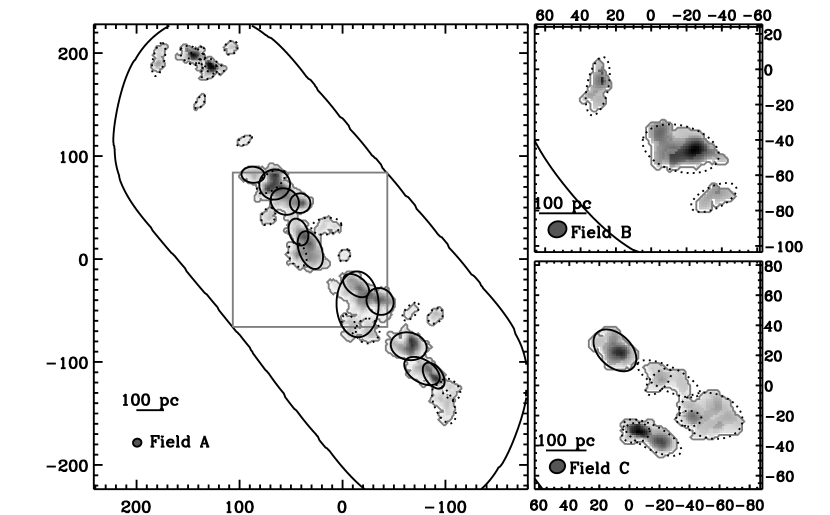
Figure 3.— Masked integrated-intensity maps of high resolution fields A–C. The black ellipses indicated the non-deconvolved major and minor axes of the molecular clouds identified by the segmentation algorithm. GMCs with sufficient signal to noise to be included in the property analysis (§4) are shown with a solid black line and low signal-to-noise clouds are shown with dotted ellipses. The gray scale runs linearly from 0 K km s^-1 (indicated with a contour) to the maximum indicated in the upper right-hand corner of each map. Axes are aligned with equatorial coordinates and are labeled in offsets measured in arcseconds from the field centers listed in Tables 1. For reference, a scale bar is plotted of projected distance in the plane of the sky and the size of the synthesized beam is depicted beside the field name. If appropriate, the edge of the surveyed region is drawn with a solid line. The square, gray box in the map for Field A indicates the region displayed in Figure 2.

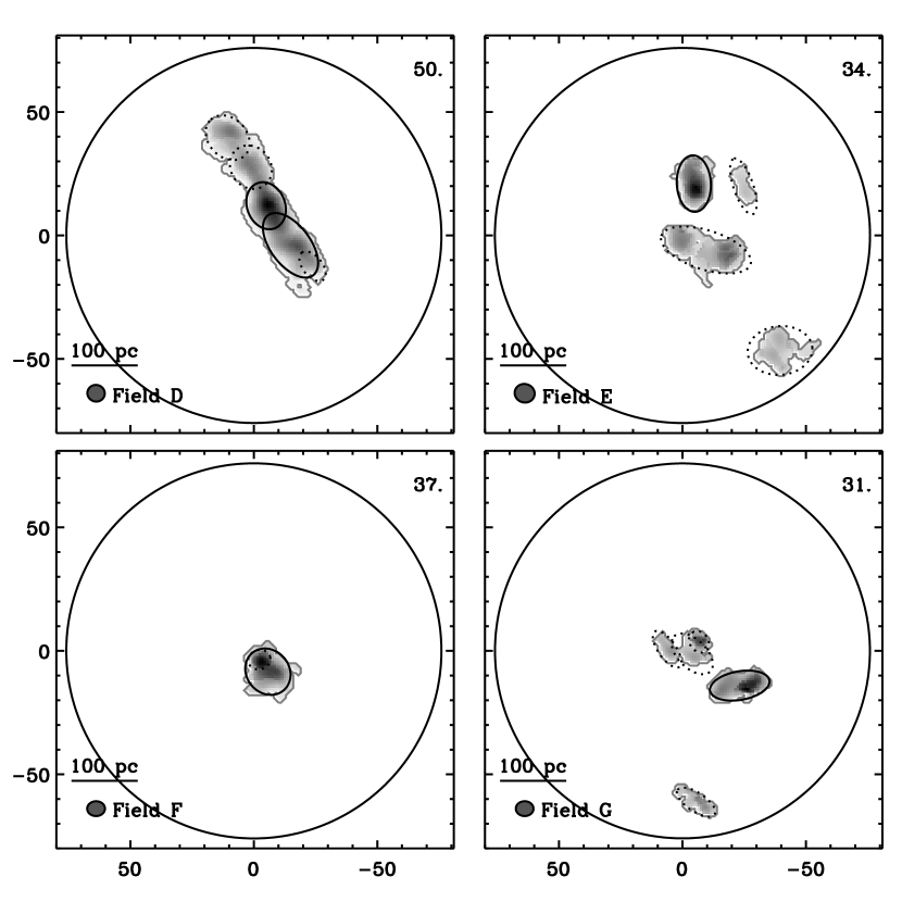
Figure 4.— As Figure 3 but for Fields D–G.

We identify emission in the data cubes from the high-resolution data (Fields A-G in Table 1) using the signal-identification method described in §3.1. Maps of the high-resolution data fields appear in Figures 3 and 4. This emission was partitioned into individual molecular clouds using the segmentation algorithm described in Rosolowsky & Leroy (2006, RL06) to separate blended emission. The segmentation algorithm is a modified watershed algorithm, related to the original CLUMPFIND (Williams et al., 1994). However, the adopted algorithm has been optimized to identify GMCs in a wide variety of observational data: the algorithm is significantly more robust to the presence of noise and does not over-segment GMCs as the original CLUMPFIND is known to do (Sheth et al., 2000). The RL06 algorithm establishes its parameters from physical scales in the data (e.g. parsecs, km s^-1) as opposed to observationally determined scales (beam and channel widths) to minimize biases in comparing catalogs with different observational properties. For the high-resolution data, the algorithm identifies 67 molecular clouds in the seven cubes.

Table 2Molecular Cloud Properties in M31

Number	Position	$M_{LUM}$	$R_{e}$	$\sigma_{v}$	$T_{max}/\sigma_{rms}$	$|\nabla v|$	$\phi_{\nabla}$
	$(^{\prime\prime},^{\prime\prime})$	($10^{4}~{}M_{\odot}$)	(pc)	(km s-1)		(km s-1 pc-1)	(∘)
High Signal-to-Noise Clouds
1	$(+322,+1246)$	55	34	4.07	17.0	0.07	$97$
2	$(+340,+1262)$	42	24	4.43	15.1	0.04	$-151$
3	$(-469,+671)$	72	52	6.29	14.9	0.12	$-66$
4	$(-238,+828)$	78	50	4.86	14.8	0.02	$67$
5	$(-300,+764)$	63	47	3.38	14.6	0.03	$132$
6	$(-256,+811)$	33	43	4.44	13.3	0.10	$125$
7	$(+2384,+709)$	33	28	2.35	13.2	0.05	$3$
8	$(-279,+782)$	25	32	5.45	12.6	0.11	$39$
9	$(+1438,+623)$	31	19	2.86	12.3	0.03	$106$
10	$(-379,+730)$	34	33	4.38	11.9	0.06	$43$
11	$(-201,+837)$	15	24	2.38	11.5	0.06	$58$
12	$(-381,+711)$	61	92	4.24	11.3	0.03	$49$
13	$(-282,+810)$	26	27	4.07	11.3	0.08	$150$
14	$(-276,+812)$	26	30	4.88	11.2	0.18	$127$
15	$(-492,+647)$	26	47	2.95	10.7	0.03	$126$
16	$(+948,-386)$	26	19	3.09	10.6	0.02	$93$
17	$(-420,+714)$	42	42	4.41	10.6	0.06	$112$
18	$(-512,+642)$	40	30	5.54	10.3	0.06	$-50$
19	$(-820,+387)$	38	40	3.99	10.3	0.08	$-145$
Low Signal-to-Noise Clouds
20	$(-254,+821)$	21	21	4.40	9.9	0.11	$-166$
21	$(-864,+329)$	31	19	2.75	9.8	0.03	$-29$
22	$(+368,+1290)$	27	25	5.39	9.7	0.08	$64$
23	$(-234,+828)$	44	34	6.19	9.7	0.17	$-88$
24	$(+351,+1278)$	24	24	5.89	9.3	0.11	$41$
25	$(+1430,+596)$	45	35	4.67	9.2	0.11	$26$
26	$(+978,-368)$	8	$\cdots$	4.64	8.8	0.16	$165$
27	$(-278,+760)$	22	28	4.13	8.7	0.09	$32$
28	$(-586,+554)$	10	$\cdots$	2.62	8.4	0.01	$112$
29	$(-129,+943)$	29	$\cdots$	6.53	8.2	0.21	$111$
30	$(-199,+837)$	3	$\cdots$	1.56	8.1	0.05	$-28$
31	$(-399,+686)$	17	37	4.70	8.0	0.13	$53$
32	$(-530,+615)$	23	42	4.51	7.8	0.07	$172$
33	$(-96,+953)$	38	27	7.03	7.7	0.14	$-172$
34	$(-38,+949)$	15	$\cdots$	2.38	7.6	0.04	$-35$
35	$(-327,+787)$	12	29	3.15	7.5	0.05	$-28$
36	$(-125,+938)$	14	$\cdots$	3.93	7.4	0.09	$103$
37	$(-285,+780)$	17	19	5.26	7.2	0.18	$102$
38	$(-232,+831)$	12	31	2.67	7.1	0.04	$-154$
39	$(-669,+519)$	37	55	2.64	6.9	0.02	$-84$
40	$(+2390,+714)$	3	$\cdots$	1.50	6.7	0.07	$-133$
41	$(+307,+1238)$	2	$\cdots$	2.42	6.7	0.06	$-134$
42	$(-933,+343)$	33	60	2.97	6.6	0.04	$39$
43	$(-907,+342)$	6	$\cdots$	3.62	6.6	0.05	$-57$
44	$(-844,+332)$	12	$\cdots$	3.65	6.5	0.06	$134$
45	$(-541,+629)$	9	25	3.42	6.4	0.04	$179$
46	$(+1000,-371)$	5	$\cdots$	1.58	6.3	0.02	$-79$
47	$(+1376,+556)$	16	35	2.08	6.3	0.04	$100$
48	$(-227,+797)$	8	$\cdots$	3.51	6.1	0.12	$18$
49	$(-515,+700)$	10	$\cdots$	2.97	6.1	0.11	$-29$
50	$(-274,+792)$	3	$\cdots$	1.74	6.1	0.06	$-27$
51	$(-235,+837)$	5	12	2.16	6.1	0.06	$168$
52	$(-703,+491)$	6	$\cdots$	2.24	6.1	0.05	$68$
53	$(-186,+870)$	2	$\cdots$	1.70	6.0	0.06	$-124$
54	$(-366,+692)$	10	$\cdots$	6.27	5.9	0.15	$77$
55	$(+980,-433)$	8	$\cdots$	5.00	5.9	0.14	$-154$
56	$(+982,-373)$	6	16	2.14	5.8	0.05	$-68$
57	$(-871,+366)$	3	$\cdots$	1.49	5.5	0.00	$73$
58	$(-225,+801)$	3	$\cdots$	2.60	5.2	0.08	$79$
59	$(-227,+794)$	4	$\cdots$	2.38	5.1	0.04	$46$
60	$(-110,+908)$	2	$\cdots$	1.79	5.1	0.04	$-8$
61	$(-359,+759)$	1	$\cdots$	0.99	5.1	0.01	$147$
62	$(-163,+961)$	4	$\cdots$	2.42	4.9	0.11	$13$
63	$(-184,+776)$	1	$\cdots$	0.98	4.8	0.04	$-59$
64	$(-473,+704)$	3	$\cdots$	1.28	4.6	0.02	$-100$
65	$(-883,+368)$	14	22	3.11	4.6	0.04	$115$
66	$(+1403,+622)$	3	$\cdots$	0.65	4.5	0.01	$-57$
67	$(-103,+953)$	4	$\cdots$	2.58	4.2	0.12	$-6$

For each of these clouds, we measure three macroscopic properties: mass, radius ($R_{e}$), line width ($\sigma_{v}$). These macroscopic properties are defined using moments of the intensity distribution (see RL06 for details). The mass of the GMCs is determined by scaling the zeroth moment (sum) of the intensity distribution by a constant CO-to-H₂ conversion factor of

$$X_{\mathrm{CO}}=2\times 10^{20}\frac{\mbox{ cm}^{-2}}{\mbox{ K km s}^{-1}}$$

(Strong & Mattox, 1996; Dame et al., 2001). Assuming a mean particle mass of 1.36$m_{\mathrm{H}}$ (Wilson & Rood, 1994) gives a mass from the integrated flux over the cloud:

$$M_{LUM}=4.4~{}M_{\odot}~{}\frac{W^{*}_{\mathrm{CO}}}{\mbox{K km s}^{-1}\mbox{pc}^{2}}.$$

The calculation uses a flux value $W^{*}_{\mathrm{CO}}$ that is extrapolated from the brightness threshold ($2\sigma_{rms}$) to 0 $\mbox{K km s}^{-1}\mbox{pc}^{2}$ using variation in $W_{\mathrm{CO}}$ as a function of threshold (Scoville et al., 1987; Rosolowsky & Leroy, 2006). RL06 demonstrate that this extrapolation practically eliminates bias in the data due to low sensitivity, though incomplete flux recovery interferometer may still affect the resulting mass estimates (§3.4). An demonstration of the extrapolation method used in this paper is shown in Figure 5.

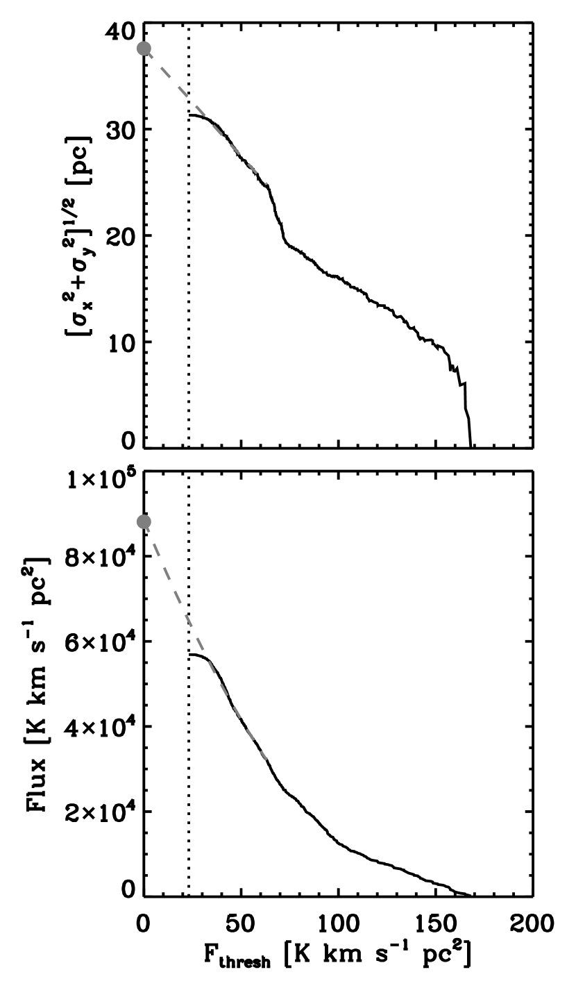
Figure 5.— Extrapolation of cloud properties (top: non-deconvolved cloud radius, bottom: flux) to the $F_{thresh}=0~{}\mbox{K km s}^{-1}\mbox{pc}^{2}$ flux threshold using the extrapolation algorithm of RL06. The extrapolation corrects for signal lost below the 2$\sigma_{rms}=23~{}\mbox{K km s}^{-1}\mbox{pc}^{2}$ clipping level (vertical dotted line). The extrapolated value is indicated with a gray dot and the extrapolation is shown as a gray dashed line. This demonstration of the extrapolation is shown for Cloud 19 in Table 2, which is the lowest significance GMC used in the analysis of cloud properties (§4).

In a similar fashion to the molecular mass, we use the moments of the emission distribution to measure the sizes and line widths of the resulting molecular clouds. Following RL06, the size is defined as the second moment of the emission distribution along the major and minor axes of the cloud: $\sigma_{maj}$ and $\sigma_{min}$ respectively. Like the total flux, the values of these moments are extrapolated to the 0 K km s^-1 pc² intensity level to minimize the effects of the brightness threshold giving $\sigma_{maj}^{*}$ and $\sigma_{min}^{*}$ (see RL06 for details). We estimate the deconvolved size of the major and minor axes by subtracting the width of the beam in quadrature. The size of the cloud is the geometric mean of the “deconvolved” major- and minor-axis sizes:

$$\sigma_{r}=\left[\sqrt{(\sigma^{*}_{maj})^{2}-\sigma_{beam}^{2}}\sqrt{(\sigma^{*}_{min})^{2}-\sigma_{beam}^{2}}\right]^{1/2}$$ (2)

The radius of the cloud is estimated by scaling $\sigma_{r}$ up by a factor of 1.91 (Solomon et al., 1987, S87). Bertoldi & McKee (1992) note that this radius estimate is insensitive to inclination and projection effects.

The rms velocity dispersion is calculated as the second moment of the emission distribution in velocity space. Again, the velocity dispersion is extrapolated to to the the 0 K km s^-1 pc² intensity level to give the corrected velocity dispersion $\sigma^{*}(v)$. The properties of the molecular clouds in the high-resolution data are summarized in Table 2. The clouds are divided into two groups: ‘high signal-to-noise clouds’ with $T_{peak}/\sigma_{rms}\geq 10$ where the macroscopic properties can be accurately recovered (see §3.4) and ‘low signal-to-noise clouds’ ($T_{peak}/\sigma_{rms}<10$) where the derived properties are suspect.

3.4. Flux Recovery

Since interferometers do not measure the total power of observed emission, they must rely upon single dish observations for accurate measurements of the CO flux. In the absence of such single-dish data, deconvolution algorithms can be used to extrapolate into the unsampled short-spacing area of the $(u,v)$ plane (Helfer et al., 2002). The accuracy of such extrapolations depends primarily on the signal-to-noise ratio of the data and to a lesser degree on the observational strategy and the structure of the object being observed. Since this work uses flux information to calculate cloud masses as well as in the moments that determine the cloud properties, flux loss affects all stages of this analysis.

We use the data from IRAM 30-m survey of M31 (Nieten et al., 2006) to quantify the amount of flux lost in each of the the observations. We report the fraction of flux in the BIMA maps relative to that found in the IRAM map in Table 1 as the column labeled $f_{rec}$. The fractions recovered range from 12% to 42%. The relatively low fraction of flux recovered is a product of two factors that affect interferometric observations: spatial filtering of GMCs (studied in Sheth et al., 2000, 2006) and the non-linear recovery of signal in the low signal-to-noise regime (explored in Helfer et al., 2002). The work of Sheth et al. (2000, 2006) found that, because of their clumpy structure, spatial filtering did not hinder the accurate measurement of GMC shapes, fluxes and properties. However, their simulations were conducted in the high signal-to-noise regime. In the low signal-to-noise regime, Helfer et al. (2002) found that even relatively compact simulated sources suffered from significant flux loss, owing to the inability for the deconvolution algorithms to isolate low-amplitude signal. These two effects (spatial filtering of GMC emission and low signal-to-noise) were studied together in RL06 who simulated BIMA C,D, and C+D observations of Milky Way GMCs (Orion, Rosette, W3/4/5) as if those GMCs were located in M31. Their work showed that accurate recovery of cloud properties required signal-to-noise ratios of $T_{max}/\sigma_{rms}\geq 10$ for less than a 20% loss in all the cloud properties. For clouds with lower significance, the flux loss is more severe. However, the dominant source of flux loss comes from clouds not detected in the observations at all, i.e. those with $T_{max}/\sigma_{rms}\lesssim 1.5$, the minimum amplitude to which the deconvolution algorithm operates. For these clouds, the deconvolution algorithm does not identify a significant local maximum for CLEANing and the cloud contributes zero flux to the deconvolved map. Such low mass clouds likely comprise most of the missing flux not seen in the interferometer data. When clouds are detected, cloud properties estimated from the observations should be relatively accurate, particularly if $T_{max}/\sigma_{rms}\geq 10$. In general, we only consider the properties of clouds in the study if this sensitivity condition is met; exceptions to this criterion will be noted. For the high-resolution data, 19 GMCs meet the signal-to-noise criterion (the ‘high signal-to-noise clouds’ in Table 2). We emphasize that for these M31 data interferometer observations act as a filter that preferentially detects GMCs, but the properties of those clouds are well-measured.

4. Molecular Cloud Properties in M31

Upon measuring a set of GMC properties for clouds in another galaxy, the immediate question is whether these clouds are similar to those found in the Milky Way. Ideally, the well-resolved clouds in the Milky Way would be analyzed using the methods of RL06 so that the results are directly comparable. However, since measuring cloud properties in the inner Galaxy requires establishing a single distance by resolving the kinematic distance ambiguity, a detailed re-analysis has not been completed to date. The next best solution is to compare the results to an existing catalog.

For comparison, we use the catalog of Solomon et al. (1987, S87) to define the population of GMCs in the inner Milky Way. The work of S87 used similar methods to calculate cloud properties though their work adopts a fundamentally different procedure for segmenting GMCs. In addition, their cloud properties are not corrected for the effects of sensitivity as are the properties derived in this study. Consequently, there may be systematic differences between their catalog and the present study. In general, the fluxes, line widths and radii of the S87 clouds will be smaller than would be derived using the methods of RL06; however, using interferometer data to observe the extragalactic clouds will reduce the fluxes, line widths and radii by a similar amount (RL06). We have rescaled the catalog of S87 to a different galactocentric solar radius: $R_{\odot}=10$ kpc to $R_{\odot}=8.5$ kpc and the CO-to-H₂ conversion factor adopted in this study. We also recalculated cloud sizes using the definition of RL06. Finally, it is noteworthy that the method of RL06 reports, in addition to unbiased values for the cloud properties, appropriate uncertainties for those properties facilitating a statistically based comparison of cloud properties in M31 to those in the Milky Way.

4.1. Scalings Among GMC Properties

Larson (1981) first demonstrated that there were power-law scalings among the properties of molecular gas clouds. That GMCs followed these scalings became well established in a series of surveys and catalogs of the CO emitting gas in the inner Milky Way (Sanders et al., 1985; Dame et al., 1986; Scoville et al., 1987, S87). Although there are several algebraically equivalent forms for expressing these relations, the most physically relevant relationships are generally agreed to be:

$$\sigma_{v}=\sigma_{0}\left(\frac{R_{e}}{\mbox{1 pc}}\right)^{0.5}$$ (3)

and

$$M=\frac{5\sigma_{v}^{2}R_{e}}{\alpha G}.$$ (4)

For the inner Milky Way, $\sigma_{0}=0.6~{}$km s^-1 and $\alpha\approx 1.5$ (S87). The first relationship is the size-line width relationship and results from the supersonic turbulent motions in the GMCs, as first suggested by Larson (1981). The constant $\alpha$ in equation 4 is the virial parameter (McKee & Zweibel, 1992) and since $\alpha<2$ in the inner Milky Way the clouds are frequently interpreted as being self-gravitating. In Figure 6, we plot these two relationships for the 19 clouds in M31 with sufficient signal to noise that their properties can be well-recovered in interferometric observations. We compare the relationships to those found in the catalog of S87.

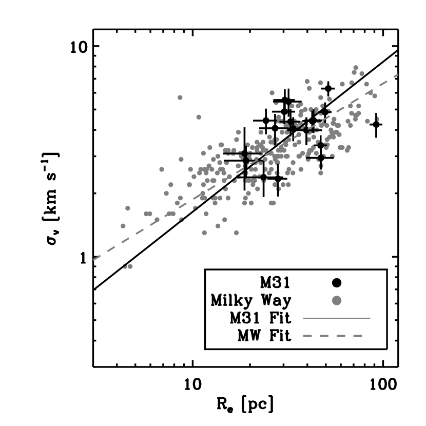
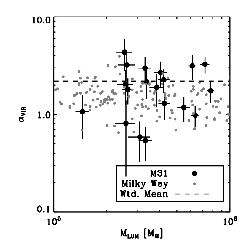
Figure 6.— (left) The size-line width relationship for the 19 clouds in M31 with sufficient signal-to-noise for accurate recovery of cloud properties. There is good agreement between clouds in M31 and those cataloged in the inner Milky Way by S87. The solid, black and dashed, gray lines are fits to the data for GMCs in M31 and the inner Milky Way respectively; the fits are statistically indistinguishable. (right) The virial parameter as a function of luminous mass. The virial parameter is roughly constant as a function of luminous mass implying a linear scaling between the luminous and virial masses of the clouds.

In both the size-line width relationship and the value of the virial parameter, there is reasonably good agreement between the GMCs in M31 and the inner Milky Way GMCs of S87. Fitting the relationship for the 19 clouds in M31 that meet the sensitivity criterion (§3.4) using the method of Akritas & Bershady (1996) gives a size-line width relationship of

$$\log\sigma_{v}=(-0.5\pm 0.3)+(0.7\pm 0.2)\log R_{e}.$$ (5)

For reference, a fit to the catalog of S87 using the same fitting method, albeit without uncertainties in the cloud properties, gives

$$\log\sigma_{v}=-0.28+0.55\log R_{e}.$$ (6)

Thus, the size-line width relationship for the molecular clouds is indistinguishable from the clouds found in the inner Milky Way. The similarity between size-line width relationship for clouds in M31 and the inner Milky Way has been reported on several occasions by other authors (Vogel et al., 1987; Wilson & Rudolph, 1993; Guélin et al., 2000; Muller & Guélin, 2003; Sheth et al., 2000), though no previous study has reported an independent fit for the clouds in M31 with well characterized uncertainties in the cloud properties.

The virial parameter for clouds in M31 is constant as a function of luminous mass. The uncertainty-weighted, mean value of the virial parameter for clouds in M31 is $\langle\alpha_{\mathrm{M31}}\rangle=2.0\pm 0.3$. For the sample of S87, $\langle\alpha_{\mathrm{MW}}\rangle=1.45$. The difference between the virial parameters is not statistically significant. Moreover, any flux loss will affect the luminous mass estimates more than the virial estimate (RL06), so our measurement of the virial parameter is at worst an upper limit. It is unlikely that the true virial parameters of M31 cloud population differs significantly from the Milky Way, provided the CO-to-H₂ conversion factor is the same for both systems. Alternatively, by assuming that the molecular clouds cataloged in this study are in the same dynamical state as are clouds in the inner Milky Way, we can justify our choice of CO-to-H₂ conversion factor. Again, the similarity of the virial parameter has been noted by several authors in previous studies (Lada et al., 1988; Guélin et al., 2000; Muller & Guélin, 2003; Guélin et al., 2004). In particular, the latter two studies find no systematic variation in the virial parameter for clouds over a large range of galactocentric radius in M31.

5. The Angular Momentum Defect of GMCs

5.1. Velocity Gradients

In addition to macroscopic properties like line width, radius and mass, interferometric observations of extragalactic GMCs can be used to measure the velocity gradients and angular momenta of the clouds. Rosolowsky et al. (2003, RPEB) analyzed the velocity gradients of GMCs in M33 to critically evaluate cloud formation theories. In this section, we analyze the velocity gradients for GMCs in M31 and compare our results to those of RPEB and the analysis of the velocity gradients in GMCs in the inner Milky Way by Koda et al. (2005).

We determine the velocity gradient by a least-squares fit of a plane to the velocity centroid surface $v_{c}(\alpha,\delta)$ – the velocity centroid measured as a function of position across the cloud. The velocity centroid and its uncertainty are determined from the first moment of velocity weighted by brightness. The coefficients of the fit determine the magnitude ($|\nabla v|$) and position angle ($\phi_{\nabla}$) of the velocity gradient for the molecular cloud (see Goodman et al., 1993, for details). The results of the fits are listed in Table 2. For purposes of this analysis, we have included all clouds, since the velocity gradient is less affected by the interferometric effects which bias the macroscopic properties (§3.4). The velocity gradient is derived from line centroids and the first moments (centroids) are much less sensitive to the low surface brightness wings of the line than are the second moments. We do exclude all measurements of the velocity gradient where the uncertainty is larger than 0.15 km s^-1 pc^-1. This upper limit was chosen from the maximum uncertainty for clouds with high signal-to-noise ($T_{max}/\sigma_{rms}>10$), including a total of 44 clouds in this portion of the analysis. Uncertainties in the derived parameters are determined from the errors in the least-squares parameters given the uncertainty in the centroid.

The magnitude of the velocity gradients range between 0 and 0.2 km s^-1 pc^-1, in good agreement with both the values and distribution found for clouds in M33 (RPEB) and the Milky Way (Koda et al., 2005). We compare the magnitude of the velocity gradient to the velocity gradient that would be expected from the orbital motion of the gas in the galactic potential, ignoring streaming motions in the spiral arms. The local galactic velocity is estimated from the tangent plane to a surface defined by the line of sight projection of the galactic rotation velocity. We use the rotation curve of Ibata et al. (2005) which is a compilation of previous CO and H I studies using updated orientation information. On average, the rotation gradient of GMCs exceeds the circular galactic gradient by a factor of 3.0.

We measured the difference between the position angle of the gradient and that of the local galactic gradient expected from circular rotation for each of the clouds. While suggesting a slight alignment with the galaxy, the distribution of this difference is not significantly different from a random distribution according to a two-sided KS test (Press et al., 1992, $P_{KS}=0.24$). This is similar to the work of Koda et al. (2005) who found a random distribution of position angles in the Milky Way GMCs but different from RPEB who found significant alignment of the gradients with the galactic rotation.

This analysis has assumed the decomposed data represent discrete clouds with independent velocity fields, and the factor of three difference between the magnitudes of the cloud and local galactic gradients supports that model. However, it is also possible that we are inappropriately decomposing a continuous gas flow into clouds and the large velocity gradients result from the change in the gas flowing into the density wave. In the presence of the radial motions that such a flow implies, the local galactic velocity gradient will change in magnitude by a factor of, at most, $\sqrt{V_{r}^{2}+V_{\theta}^{2}}/V_{\theta}$ and in position angle by $\tan^{-1}(V_{r}/V_{\theta})$ where $V_{r}$ and $V_{\theta}$ are the radial and azimuthal components of the gas flow. For gas in M31, $V_{r}/V_{\theta}\sim 0.1$ (Braun, 1991) so these changes will not be significant and the factor of three excess of cloud gradient magnitude over the local rotational gradient implies discontinuous velocity fields. Moreover, any changes should be systematic in nature, and the large range of position angles actually observed implies we are measuring the velocity gradients of discrete objects.

5.2. Angular Momentum

While the magnitudes of the velocity gradients of the clouds are larger than the local rotation in the galaxy, the implied angular momentum of the GMCs is significantly smaller than that of an equivalent mass of atomic gas orbiting in the galactic gravitational potential at the GMC’s position. The specific angular momentum for a cloud of gas with velocity gradient magnitude $|\nabla v|$ is $j_{GMC}=\beta|\nabla v|R_{e}^{2}$ where $\beta=0.4\pm 0.1$ for a wide range of density distributions undergoing uniform rotation (Phillips, 1999). If the velocity gradient arises solely from the turbulent motions in the cloud, $\beta$ is likely 2–3 times smaller (Burkert & Bodenheimer, 2000).

It is unlikely that the high galactic inclination affects the results. The near-random distribution of the position angles implies that the cloud angular momentum vectors are similarly close to random which would require scaling the angular momentum up by a factor of $4/\pi$ on average (RPEB). A turbulent origin for the velocity gradients would not necessitate any correction. Since any correction would be small, we make no correction for the orientation of the clouds.

For the clouds in the velocity gradient analysis, the mean angular momentum is $(36\pm 3)$ pc km s^-1 for a solid body rotator and 2–3 times smaller for the angular momentum of turbulent flows, comparable to the results for other systems (RPEB, Koda et al., 2005). We compare this to the angular momentum of progenitor material for the GMCs. The angular momentum of the gas in the galactic potential is given by RPEB (equivalent to Mestel, 1966)

$$j_{gal}=\eta\Delta R_{gal}^{2}\frac{1}{R_{gal}}\frac{d}{dR_{gal}}(R_{gal}V_{\theta})$$ (7)

where $\eta$ is a form factor equal to 1/4 for a contraction of a uniform circular disk of material of radius $\Delta R_{gal}$. The length, $\Delta R_{gal}$, is the range of galactocentric radii over which material is accumulated to form a GMC. The minimum value of $\Delta R_{gal}$ is set by the mass of the GMC under consideration and the surface density of gas that could comprise the progenitor material: $M_{GMC}=\pi\Sigma_{prog}\Delta R_{gal}^{2}$. We take $\Sigma_{prog}=10~{}M_{\odot}\mbox{ pc}^{-2}$ (Nieten et al., 2006), including their estimates of both atomic and molecular material since small molecular clouds seen in CO may be progenitor material for the larger GMCs. From the measured masses of GMCs and locations of GMCs, we calculate $\Delta R_{gal}$ and the galactic shear from the rotation curve of Ibata et al. (2005). The mean value of $\langle j_{gal}\rangle=(63\pm 5)\mbox{ pc km s}^{-1}$ for the clouds in the sample. On a cloud by cloud basis, the angular momentum of the galactic material is only a factor of 1.7 larger than the that of the GMCs, significantly smaller than the difference found in M33 where $\langle j_{gal}/j_{GMC}\rangle=5$. The smaller margin is primarily due to the lower shear in M31, reducing $j_{gal}$ by a factor of 4 compared to that found for the clouds in M33 whereas the velocity gradients are comparable in the two systems. Similarly, the cloud properties and gradients for clouds in the Milky Way are comparable to the clouds in M31 (Koda et al., 2005), but the shear is much larger in the inner Milky Way compared to the 11-kpc arm of M31. Consequently, the discrepancy between the angular momentum of progenitor material and the resulting GMCs is also larger in the inner Milky Way than it is in M31 (see Blitz, 1993). The angular momentum defect for the M31 clouds is likely significant: the factor of 1.7 difference should be regarded as a minimum value since attributing the velocity gradients to turbulence or accumulating the progenitor material from a larger range of galactocentric radius will appreciably increase the margin.

These results suggest a broad similarity between GMCs in M31 and the other disk galaxies in the Local Group. The primary goal of studying the velocity structure within the GMCs is to relate their angular momentum to that of the ISM as a whole to evaluate formation mechanisms. The angular momentum defect between GMCs and the ISM is common among the studied systems (Blitz, 1993, RPEB) and suggests the importance of braking in molecular cloud formation. Kim et al. (2003) study the role of magnetic effects at removing angular momentum from forming clouds and conclude that magnetic effects can reduce the angular momentum to observed values. Their unmagnetized simulations show no significant reduction in cloud angular momentum, although the density enhancements that represent proto-GMCs show $j_{gal}/j_{gmc}\sim 2$, similar to the observed minimum value found in M31. The relatively low-shear environment does not necessarily require magnetic braking to produce the observed cloud angular momenta, though our measurement of $j_{gal}/j_{gmc}$ likely significantly underestimates the true value.

6. Galactic Environment and GMC Properties

With respect to their macroscopic properties and velocity gradients, GMCs in the 11-kpc, star-forming arm in M31 appears indistinguishable from the molecular clouds in the inner Milky Way. As our knowledge of GMCs in other galaxies grows, it becomes more apparent that such detailed agreement in the properties of GMCs is not universal and may actually represent exceptional cases (Blitz et al., 2006). Given the differences measured among extragalactic cloud populations, the most pressing question is: what physical mechanisms regulate the observed differences in GMCs properties? These mechanisms must couple the GMCs to the ISM on much larger scales, and future studies will examine the nature of this coupling in more detail.

The similarity between GMCs in M31 and the Milky Way offers a useful point of reference for studying the relationship between the galactic ISM and GMCs. Finding environmental properties that vary significantly between the two systems while GMC properties remain the same would imply those properties are irrelevant to the regulation of molecular cloud properties. Several features of the galactic environment are thought to play a role in regulating the structure of the cold ISM and the properties of GMCs. Here, we review several of these features and note the degree of similarity to the local Milky Way:

• Interstellar Radiation Field — The interstellar radiation field in M31 has been previously noted to be poor in the ultraviolet relative to the Milky Way (Cesarsky et al., 1998), though the M31 field may be significantly enhanced in the star-forming spiral arm imaged in the CO observations. Indeed, work by Rodriguez-Fernandez et al. (2006) study [C II] emission in the star forming arms at $R_{gal}\sim 10$ kpc and note that the far ultraviolet field is consistent with being 100 times the local interstellar value (i.e. $G_{0}=10^{2}$) around molecular clouds. Thus, the observed FUV deficiency likely does not characterize the molecule rich region of the galaxy and the radiation environment is similar to clouds in the Milky Way.

• Metallicity — The gas phase metallicity from H II regions in M31 at $R_{gal}=10$ kpc is approximately [O/H]-[O/H]_⊙=0.0 dex with significant scatter, up to $\sim$ 0.2 dex (Dennefeld & Kunth, 1981; Blair et al., 1982). The region shows no signs of being significantly enriched or depleted relative to the solar neighborhood.

• Dynamics — The Toomre $Q$ parameter is frequently used to evaluate the stability of galactic disks with respect to the formation of self-gravitating structures. The parameter is defined as

  $$Q\equiv\frac{\kappa\sigma_{g}}{\pi G\Sigma_{g}}$$ (8)

  where $\kappa$ is the epicyclic frequency, $\sigma_{g}$ is the one-dimensional gas velocity dispersion and $\Sigma_{g}$ the surface density of the gas in the disk. Most star-forming regions of galactic disks show $Q\approx 1.5$ (Martin & Kennicutt, 2001) and this region of M31 is no exception. For the rotation curve of Ibata et al. (2005), $\kappa=0.03~{}\mbox{km s}^{-1}\mbox{ pc}^{-1}$. We take $\Sigma_{g}\approx 10~{}M_{\odot}$ (Nieten et al., 2006). Finally, we take $\sigma_{g}\approx 8\mbox{ km s}^{-1}$ from Unwin (1983). Combining these data give $Q\approx 1.8$, well within the range of values observed in most galaxies and approximately the same value found in the solar neighborhood.

• Midplane Density — We can also compare the midplane particle density of this region in M31 to the solar neighborhood. The mean particle density is important for regulating thermal structure of the ISM and the formation of the cold medium (Wolfire et al., 2003). Adopting a gas scale height of 340 pc for this region of M31 (Braun, 1991) gives $\langle n\rangle=0.5\mbox{ cm}^{-3}$ in the spiral arm region, but falling to $\langle n\rangle=0.1\mbox{ cm}^{-3}$ outside the arm. These densities are smaller than that found in the solar neighborhood ($\langle n\rangle=1.0\mbox{ cm}^{-3}$, Wolfire et al., 2003).

The properties of the ISM in this region of M31 appear, at least superficially, similar to those found in the solar neighborhood. Hence, the derived similarity of molecular clouds in the two galaxies is not surprising. The only property that appears like it may be significantly different between the two environments is the midplane particle density in the neutral medium. If the difference is significant, the constancy of the GMC properties suggests that the particle density may be important in regulating the fraction of material found in the cold, neutral ISM but perhaps not the properties of individual GMCs. While this environmental similarity does not isolate any irrelevant physical processes, noting the similarity in both clouds and environments illustrates that similar galactic environments do indeed produce similar GMCs.

7. Summary and Conclusions

This paper has presented BIMA millimeter interferometer observations of ¹²CO($J=1\to 0$) emission from giant molecular clouds (GMCs) along a spiral arm at $R_{gal}\approx 10$ kpc in M31. The observations were conducted in two parts: a low-resolution survey using the compact (D) configuration of the array and a high-resolution, follow-up study using a more extended (C) configuration of the array. All data from the study were segmented and analyzed with the analysis algorithms of Rosolowsky & Leroy (2006), which correct the observational biases imprinted on the data by having relatively low signal-to-noise and marginally resolving the GMCs. The C-array follow-up spans 7.4 kpc² finding 67 clouds. We report the following conclusions:

1. The GMC population is very similar to that found in the inner Milky Way. Both the size-line width relationship and distribution of virial parameters are statistically indistinguishable from those derived from the population of clouds in the inner Milky Way. This confirms the work of several authors (Vogel et al., 1987; Wilson & Rudolph, 1993; Guélin et al., 2000; Muller & Guélin, 2003; Sheth et al., 2000) while using techniques that correct for the biases imprinted by using interferometric observations.

2. We measured the velocity gradients and angular momenta across the GMCs. Like the Milky Way and M33, there is significantly more angular momentum in possible progenitor material than in the resulting GMCs, though the discrepancy is smallest in M31 owing to the relatively low galactic shear at large galactocentric radii. All three systems suggest braking mechanisms act during the process of cloud formation to dissipate angular momentum.

3. The galactic environment in M31 where the GMCs are found is similar in most respects that of the solar neighborhood and inner Milky Way. That GMCs in both environments are similar is consistent with the idea that the galactic environment regulates GMC properties. In systems where the galactic environment differs significantly from those studied here, the GMC properties are found to be different (e.g., Blitz et al., 2006).

References

- Akritas & Bershady (1996) Akritas, M. G. & Bershady, M. A. 1996, ApJ, 470, 706
- Bertoldi & McKee (1992) Bertoldi, F. & McKee, C. F. 1992, ApJ, 395, 140
- Blair et al. (1982) Blair, W. P., Kirshner, R. P., & Chevalier, R. A. 1982, ApJ, 254, 50
- Blitz (1993) Blitz, L. 1993, in Protostars and Planets III, 125–161
- Blitz et al. (2006) Blitz, L., Fukui, Y., Kawamura, A., Leroy, A., Mizuno, N., & Rosolowsky, E. 2006, in Protostars and Planets V, 1–18
- Braun (1991) Braun, R. 1991, ApJ, 372, 54
- Burkert & Bodenheimer (2000) Burkert, A. & Bodenheimer, P. 2000, ApJ, 543, 822
- Cesarsky et al. (1998) Cesarsky, D., Lequeux, J., Pagani, L., Ryter, C., Loinard, L., & Sauvage, M. 1998, A&A, 337, L35
- Dame et al. (1986) Dame, T. M., Elmegreen, B. G., Cohen, R. S., & Thaddeus, P. 1986, ApJ, 305, 892
- Dame et al. (2001) Dame, T. M., Hartmann, D., & Thaddeus, P. 2001, ApJ, 547, 792
- Dame et al. (1993) Dame, T. M., Koper, E., Israel, F. P., & Thaddeus, P. 1993, ApJ, 418, 730
- Dennefeld & Kunth (1981) Dennefeld, M. & Kunth, D. 1981, AJ, 86, 989
- Engargiola et al. (2003) Engargiola, G., Plambeck, R. L., Rosolowsky, E., & Blitz, L. 2003, ApJS, 149, 343
- Freedman & Madore (1990) Freedman, W. L. & Madore, B. F. 1990, ApJ, 365, 186
- Goodman et al. (1993) Goodman, A. A., Benson, P. J., Fuller, G. A., & Myers, P. C. 1993, ApJ, 406, 528
- Guélin et al. (2004) Guélin, M., Muller, S., Nieten, C., Neininger, N., Ungerechts, H., Lucas, R., & Wielebinski, R. 2004, in The Dense Interstellar Medium in Galaxies, 121–+
- Guélin et al. (2000) Guélin, M., Nieten, C., Neininger, N., Muller, S., Lucas, R., Ungerechts, H., & Wielebinski, R. 2000, in Proceedings 232. WE-Heraeus Seminar, 15–20
- Helfer et al. (2003) Helfer, T. T., Thornley, M. D., Regan, M. W., Wong, T., Sheth, K., Vogel, S. N., Blitz, L., & Bock, D. C.-J. 2003, ApJS, 145, 259
- Helfer et al. (2002) Helfer, T. T., Vogel, S. N., Lugten, J. B., & Teuben, P. J. 2002, PASP, 114, 350
- Ibata et al. (2005) Ibata, R., Chapman, S., Ferguson, A. M. N., Lewis, G., Irwin, M., & Tanvir, N. 2005, ApJ, 634, 287
- Ichikawa et al. (1985) Ichikawa, T., Nakano, M., Tanaka, Y. D., Saito, M., Nakai, N., Sofue, Y., & Kaifu, N. 1985, PASJ, 37, 439
- Kim et al. (2003) Kim, W., Ostriker, E. C., & Stone, J. M. 2003, ApJ, 599, 1157
- Koda et al. (2005) Koda, J., Sawada, T., Hasegawa, T., & Scoville, N. 2005, ArXiv Astrophysics e-prints
- Kramer et al. (1998) Kramer, C., Stutzki, J., Rohrig, R., & Corneliussen, U. 1998, A&A, 329, 249
- Lada et al. (1988) Lada, C. J., Margulis, M., Sofue, Y., Nakai, N., & Handa, T. 1988, ApJ, 328, 143
- Larson (1981) Larson, R. B. 1981, MNRAS, 194, 809
- Loinard & Allen (1998) Loinard, L. & Allen, R. J. 1998, ApJ, 499, 227
- Loinard et al. (1999) Loinard, L., Dame, T. M., Heyer, M. H., Lequeux, J., & Thaddeus, P. 1999, A&A, 351, 1087
- Martin & Kennicutt (2001) Martin, C. L. & Kennicutt, R. C. 2001, ApJ, 555, 301
- McKee & Zweibel (1992) McKee, C. F. & Zweibel, E. G. 1992, ApJ, 399, 551
- Melchior et al. (2000) Melchior, A.-L., Viallefond, F., Guélin, M., & Neininger, N. 2000, MNRAS, 312, L29
- Mestel (1966) Mestel, L. 1966, MNRAS, 131, 307
- Mizuno et al. (2001a) Mizuno, N., Rubio, M., Mizuno, A., Yamaguchi, R., Onishi, T., & Fukui, Y. 2001a, PASJ, 53, L45
- Mizuno et al. (2001b) Mizuno, N., Yamaguchi, R., Mizuno, A., Rubio, M., Abe, R., Saito, H., Onishi, T., Yonekura, Y., Yamaguchi, N., Ogawa, H., & Fukui, Y. 2001b, PASJ, 53, 971
- Muller (2003) Muller, S. 2003, Ph.D. Thesis
- Muller & Guélin (2003) Muller, S. & Guélin, M. 2003, in SF2A-2003: Semaine de l’Astrophysique Francaise, 279–+
- Nieten et al. (2006) Nieten, C., Neininger, N., Guélin, M., Berkhuijsen, E., & Beck, R. 2006, A&A, 000, in press
- Phillips (1999) Phillips, J. P. 1999, A&AS, 134, 241
- Press et al. (1992) Press, W. H., Teukolsky, S. A., Vetterling, W. T., & Flannery, B. P. 1992, Numerical recipes in C. The art of scientific computing (Cambridge: University Press, —c1992, 2nd ed.)
- Rodriguez-Fernandez et al. (2006) Rodriguez-Fernandez, N. J., Braine, J., Brouillet, N., & Combes, F. 2006, ArXiv Astrophysics e-prints
- Rosolowsky & Leroy (2006) Rosolowsky, E. & Leroy, A. 2006, PASP, 118, 590
- Rosolowsky et al. (2003) Rosolowsky, E. W., Plambeck, R., Engargiola, G., & Blitz, L. 2003, ApJ, 599, 258
- Sanders et al. (1985) Sanders, D. B., Scoville, N. Z., & Solomon, P. M. 1985, ApJ, 289, 373
- Sault et al. (1995) Sault, R. J., Teuben, P. J., & Wright, M. C. H. 1995, in ASP Conf. Ser. 77: Astronomical Data Analysis Software and Systems IV, 433–+
- Scoville et al. (1987) Scoville, N. Z., Yun, M. S., Sanders, D. B., Clemens, D. P., & Waller, W. H. 1987, ApJS, 63, 821
- Sheth et al. (2006) Sheth, K., Vogel, S., Wilson, C., & Dame, T. 2006, ApJ, submitted
- Sheth et al. (2000) Sheth, K., Vogel, S. N., Wilson, C. D., & Dame, T. M. 2000, in The interstellar medium in M31 and M33. Proceedings 232. WE-Heraeus Seminar, 22-25 May 2000, Bad Honnef, Germany. Edited by Elly M. Berkhuijsen, Rainer Beck, and Rene A. M. Walterbos. Shaker, Aachen, 2000, p. 37-40, 37–40
- Solomon et al. (1987) Solomon, P. M., Rivolo, A. R., Barrett, J., & Yahil, A. 1987, ApJ, 319, 730
- Strong & Mattox (1996) Strong, A. W. & Mattox, J. R. 1996, A&A, 308, L21
- Stutzki & Güsten (1990) Stutzki, J. & Güsten, R. 1990, ApJ, 356, 513
- Taylor et al. (1999) Taylor, C. L., Hüttemeister, S., Klein, U., & Greve, A. 1999, A&A, 349, 424
- Unwin (1983) Unwin, S. C. 1983, MNRAS, 205, 773
- Vogel et al. (1987) Vogel, S. N., Boulanger, F., & Ball, R. 1987, ApJ, 321, L145
- Walterbos & Kennicutt (1988) Walterbos, R. A. M. & Kennicutt, Jr., R. C. 1988, A&A, 198, 61
- Welch et al. (1996) Welch, W. J., Thornton, D. D., Plambeck, R. L., Wright, M. C. H., Lugten, J., Urry, L., Fleming, M., Hoffman, W., Hudson, J., Lum, W. T., Forster, J. . R., Thatte, N., Zhang, X., Zivanovic, S., Snyder, L., Crutcher, R., Lo, K. Y., Wakker, B., Stupar, M., Sault, R., Miao, Y., Rao, R., Wan, K., Dickel, H. R., Blitz, L., Vogel, S. N., Mundy, L., Erickson, W., Teuben, P. J., Morgan, J., Helfer, T., Looney, L., de Gues, E., Grossman, A., Howe, J. E., Pound, M., & Regan, M. 1996, PASP, 108, 93
- Williams et al. (1994) Williams, J. P., de Geus, E. J., & Blitz, L. 1994, ApJ, 428, 693
- Wilson (1994) Wilson, C. D. 1994, ApJ, 434, L11
- Wilson & Rudolph (1993) Wilson, C. D. & Rudolph, A. L. 1993, ApJ, 406, 477
- Wilson & Scoville (1990) Wilson, C. D. & Scoville, N. 1990, ApJ, 363, 435
- Wilson & Rood (1994) Wilson, T. L. & Rood, R. 1994, ARA&A, 32, 191
- Wolfire et al. (2003) Wolfire, M. G., McKee, C. F., Hollenbach, D., & Tielens, A. G. G. M. 2003, ApJ, 587, 278