A fast hybrid algorithm for exoplanetary transit searches

Abstract

We present a fast and efficient hybrid algorithm for selecting exoplanetary candidates from wide-field transit surveys. Our method is based on the widely-used SysRem and Box Least-Squares (BLS) algorithms. Patterns of systematic error that are common to all stars on the frame are mapped and eliminated using the SysRem algorithm. The remaining systematic errors caused by spatially localised flat-fielding and other errors are quantified using a boxcar-smoothing method. We show that the dimensions of the search-parameter space can be reduced greatly by carrying out an initial BLS search on a coarse grid of reduced dimensions, followed by Newton-Raphson refinement of the transit parameters in the vicinity of the most significant solutions. We illustrate the method’s operation by applying it to data from one field of the SuperWASP survey, comprising 2300 observations of 7840 stars brighter than $V=13.0$. We identify 11 likely transit candidates. We reject stars that exhibit significant ellipsoidal variations indicative of a stellar-mass companion. We use colours and proper motions from the 2MASS and USNO-B1.0 surveys to estimate the stellar parameters and the companion radius. We find that two stars showing unambiguous transit signals pass all these tests, and so qualify for detailed high-resolution spectroscopic follow-up.

1 Introduction

Among the 194 extra-solar planets discovered in the last decade, the “hot Jupiters” currently present the greatest challenges to understanding and the greatest observational rewards. Efforts to explain their origin have transformed theories of planetary-system formation. Do these planets form via gravitational instability in cold discs, or must they form by core accretion beyond the ice boundary, where ice mantles on dust grains allow rapid agglomeration of a massive core of heavy elements? How rapidly do they migrate inwards through a massive protoplanetary disc, and what mechanism halts the migration?

The subset of these planets that transit their parent stars are of key importance in addressing these questions, because they are the only planets whose radii and masses can be determined directly. The first such discovery (Charbonneau et al., 2000) confirmed the gas-giant nature of the hot Jupiters; indeed the inflated radius of HD 209458b continues to challenge our understanding of exoplanetary interior structure. Subsequent discoveries have presented further surprises. The apparent correlation between planet mass and minimum survivable orbital separation among the known transiting planets offers important clues to the “stopping mechanism” for inward orbital migration of newly-formed giant planets in protoplanetary discs (Mazeh et al., 2005). The high core mass of the recently-discovered Saturn-mass planet orbiting HD 149026 (Sato et al. 2005) presents difficulties for models of planet formation via gravitational instability. Spitzer observations of the secondary eclipses of TReS-1b, HD 209458b and HD189733b have provided the first estimates of the temperatures in these planets’ cloud decks (Charbonneau et al. 2005; Deming et al. 2005; Deming et al. 2006).

To date, however, only ten such planets have been discovered. Three of the ten have been found via targeted radial-velocity searches, the other six through large-scale photometric surveys for transit events. The primary goal of the SuperWASP project (Pollacco et al. 2006) is to discover bright, new transiting exoplanets in sufficiently large numbers that we can place studies of their mass-radius relation, and the suspected relationship between minimum orbital distance and planet mass, on a secure statistical footing. SuperWASP’s “shallow-but-wide” approach to transit hunting is designed to find planets that are not only sufficiently bright ($10<V<13.0$) for high-precision radial-velocity follow-up studies to be feasible on telescopes of modest aperture, but also for detailed follow-up studies such as transmission spectroscopy during transits, and Spitzer secondary-eclipse observations. Only five of the ten presently-known transiting planets orbit stars brighter than $V=14$ and so have such strong follow-up potential.

Here we present a methodology used in the search for exoplanetary transit candidates in data from the first year of SuperWASP operation. We employ the SysRem algorithm of Tamuz et al. (2005) to identify and remove patterns of correlated systematic error from the stellar light-curves. We present a refined version of the Box Least-Squares (BLS) algorithm of Kovács et al. (2002), which permits a fast grid search and efficient refinement of the most promising solutions without binning the data. Using simulated transits injected into real SuperWASP data we develop a filtering strategy to optimise and quantify the recovery rate and false-alarm probability as functions of stellar magnitude and transit depth. We develop simple plausibility tests for transit candidates, using the transit duration and depth to estimate the mass of the parent star and the radius of the planet. We mine publicly-available catalogues to obtain the $V-K$ colours, proper motions and other properties of the host stars. Combined with the transit durations and depths, these give improved physical parameters of each system and help us to identify the most promising candidates for spectroscopic follow-up observations.

2 Instrumentation and Observations

The SuperWASP camera array, located at the Observatorio del Roque de los Muchachos on La Palma, Canary Islands, consists of five 200mm f/1.8 Canon lenses each with an Andor CCD array of $2048^{2}$ 13.5$\mu$m pixels, giving a field of view 7.8 degrees square for each camera. By cycling through a sequence of 7 or 8 fields located within 4 hours of the meridian, at field centres separated by one hour right ascension, SuperWASP monitored up to 8% of the entire sky for between 4 and 8 hours each night during the 2004 observing season. The average interval between visits to each field was 6 minutes. Each exposure was of 30s duration, and was taken without filters.

Between 2004 May and September, the five SuperWASP cameras secured light-curves of some $2\times 10^{5}$ stars brighter than $V=13$. The long-term precision of the data (determined from the RMS scatter of individual data points for non-variable stars) is 0.004 mag at $V=9.5$, degrading to 0.01 mag at $V=12.3$. Our sampling rate and run duration guarantee that 4 or more transits should have been observed in 90% of all systems with periods less than 5 days, and 100% of all systems with periods less than 4 days, though some incompleteness is expected at periods very close to integer multiples of 1 day.

3 Data reduction

The data were reduced using the SuperWASP pipeline. The pipeline carries out an initial statistical analysis of the raw images, classifying them as bias frames, flat fields, dark frames or object frames. The bias frames are combined using optimally weighted averaging with outlier rejection. Automated sequences of flat fields secured at dawn and dusk are corrected for sky illumination gradients and combined using an optimal algorithm that maps and corrects for the pattern introduced by the finite opening and closing time of the iris shutter on each camera.

Science frames are bias-subtracted, corrected for shutter travel time and corrected for pixel-to-pixel sensitivity variations and vignetting using the flat-field exposures. Flat fields from different nights are combined using a algorithm in which the weights of older flat field frames decay on a timescale of 14 days. A catalogue of objects on each frame is constructed using extractor, the Starlink implementation of the SExtractor (Bertin & Arnouts, 1996) source detection software. An automated field recognition algorithm identifies the objects on the frame with their counterparts in the tycho-2 catalogue (Høg et al., 2000)and establishes an astrometric solution with an RMS precision of 0.1 to 0.2 pixel.

Aperture photmetry is then carried out at the positions on each CCD image of all objects in the USNO-B1.0 catalogue (Monet et al., 2003) with second-epoch red magnitudes brighter than 15.0. Fluxes are measures in three apertures with radii of 2.5, 3.5 and 4.5 pixels. The ratios between the fluxes in different pairs of apertures yield a “blending index” which quantifies image morphology, and is used to flag blended stellar images and extended, non-stellar objects. Individual objects are allocated SuperWASP identifiers of the form “1SWASP J$hhmmss.ss+ddmmss.s$”, which are based on their USNO-B1.0 coordinates for equinox J2000.0 and epoch J2000.0.

The resulting fluxes are corrected for primary and secondary extinction, and the zero-point for each frame is tied to a network of local secondary standards in each field, whose magnitudes are derived from WASP fluxes transformed via a colour equation relating instrumental magnitudes to tycho-2 $V$ magnitudes. The resulting fluxes are stored in the SuperWASP Data Archive at the University of Leicester. The corresponding transformed magnitudes for all objects in each field are referred to as “WASP $V$” magnitudes throughout this paper.

3.1 Sample selection and survey completeness

The field chosen for development and testing of the transit search algorithm is centred at $\alpha_{2000}=01$h 43m, $\delta_{2000}=+31^{\circ}$ 26’. A search of the WASP archive, centred on this position and covering the full 7.8^∘-square field of view of the camera, yielded light-curves of 7840 stars brighter than WASP $V=13$ for which a catalogue query indicated that the light-curves comprised more than 500 valid photometric data points. Indeed most of the objects in this field had more than 2000 valid photometric measurements. The maxipara 2 mum number of valid observations in any light-curve was 2301. The resulting set of light-curves was loaded into a rectangular matrix of 7840 light-curves by 2301 observations for further processing.

The expected number of transits present in the observed light-curve of any given star depends on the sampling pattern of the observations and the period and phase of the transit cycle. In Fig. 1 we plot the probability of $N_{t}$ or more transits being present in the data, as a function of orbital period. We consider a transit as having been “observed” if data have been obtained within the phase ranges $\phi<0.1w/P$ or $\phi>1-0.1w/p$, where $w$ is the expected transit duration as described at the start of Section 5 and $P$ is the orbital period. The regular sampling pattern on most nights of acceptable quality generally ensures that at least 40 percent of a given transit event must be well-observed if it is to be counted according to this criterion. For the field studied here, the prospects of observing at least three transits is 70% or better at periods less than 3.5 days.

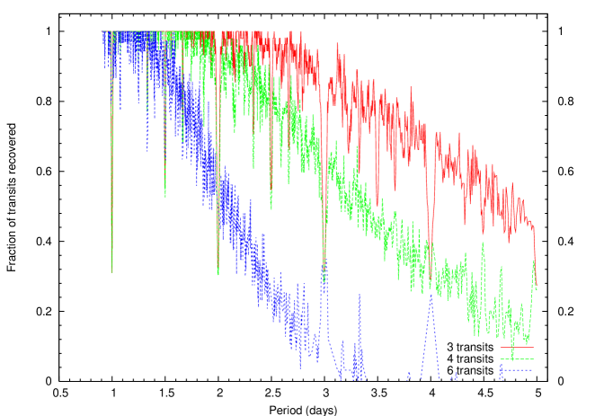
Figure 1: Probability of observing more than $N_{t}$ transit events in the 2004 data from the field centred at RA = 01h 43m, Dec = +31^∘ 26^′, as a function of orbital period. For periods less than 5 days, the probability of observing 3 or more transits is at least 50 percent, except at periods close to integer and half-integer numbers of days.

4 Systematic error removal

The reduced data from the pipeline inevitably contain low-level systematic errors. In this section we describe a coarse initial decorrelation and application of the SysRem algorithm of Tamuz et al. (2005). Before modelling and removing patterns of correlated error we perform a coarse initial decorrelation by referencing each star’s magnitude to its own mean, removing small night-to-night and frame-to-frame differences in the zero-point, and measuring the additional, independent variance components introduced in individual stars by their intrinsic variablility and in some observations by patchy cloud.

4.1 Coarse decorrelation

We start with a two-dimensional array $m_{ij}$ of processed stellar magnitudes from the pipeline. The first index $i$ denotes a single CCD frame within the entire season’s data. The second index labels an individual star. We compute the mean magnitude of each star:

$$\hat{m}_{j}=\frac{\sum_{i}m_{ij}w_{ij}}{\sum_{i}w_{ij}}$$ (1)

where the weights $w_{ij}$ incorporate both the formal variance $\sigma^{2}_{ij}$ calculated by the pipeline from the stellar and sky-background fluxes, and an additional systematic variance component $\sigma^{2}_{t(i)}$ introduced in individual frames by passing wisps of cloud, Sahara dust events and other transient phenomena which degrade the extinction correction:

$$w_{ij}=\frac{1}{\sigma^{2}_{ij}+\sigma^{2}_{t(i)}}.$$ (2)

Data points from frames of dubious quality are thus down-weighted. The weight is set to zero for any data point flagged by the pipeline as either missing or bad.

The zero-point correction for each frame $i$ follows:

$$\hat{z}_{i}=\frac{\sum_{j}(m_{ij}-\hat{m}_{j})u_{ij}}{\sum_{j}u_{ij}}$$ (3)

In this case the weights are defined as

$$u_{ij}=\frac{1}{\sigma^{2}_{ij}+\sigma^{2}_{s(j)}},$$ (4)

where $\sigma^{2}_{s(j)}$ is an additional variance caused by intrinsic stellar variability. This down-weights variable stars in the calculation of the zero-point offset for each frame.

Initially we set $\sigma^{2}_{t(i)}=\sigma^{2}_{s(j)}=0$, and compute the average magnitude $\hat{m}_{j}$ for every star $j$ and the zero-point offset $\hat{z}_{i}$ for every frame.

To determine the additional variance of $\sigma^{2}_{s(j)}$ for the intrinsic variability of a given star $j$ from the data themselves, we use a maximum-likelihood approach. We define a data vector $\vec{X}=\{m_{ij},i=1...n\}$ containing the light-curve of star $j$, and a model $\vec{\mu}=\{\hat{m}_{j}+\hat{z}_{i},i=1...n\}$. If both sets of errors are gaussian, then the probability of the $i$th individual observation is

$$P(\vec{X}_{i}|\vec{\mu}_{i})=\frac{1}{\sqrt{2\pi}\sqrt{\sigma^{2}_{ij}+\sigma^{2}_{t(i)}+\sigma^{2}_{s(j)}}}\exp\left(-\frac{(m_{ij}-\hat{m}_{j}-\hat{z}_{i})^{2}}{2(\sigma^{2}_{ij}+\sigma^{2}_{t(i)}+\sigma^{2}_{s(j)})}\right).$$

The likelihood of the entire data vector for star $j$ given the model is

$$L(\vec{\mu})=(2\pi)^{-n/2}\prod_{i}\left(\frac{1}{\sqrt{\sigma^{2}_{ij}+\sigma^{2}_{t(i)}+\sigma^{2}_{s(j)}}}\right)\exp\left({-\frac{1}{2}\chi^{2}}\right).$$

where

$$\chi^{2}=\sum_{i}\frac{(m_{ij}-\hat{m}_{j}-\hat{z}_{i})^{2}}{\sigma^{2}_{ij}+\sigma^{2}_{t(i)}+\sigma^{2}_{s(j)}}.$$

Taking logs and differentiating, we find that the maximum-likelihood value of $\sigma_{s(j)}$ satisfies

$$\frac{d}{d\sigma_{s(j)}}\left(\chi^{2}+\sum_{i}\ln(\sigma^{2}_{ij}+\sigma^{2}_{t(i)}+\sigma^{2}_{s(j)})\right)$$

$$=2\sigma_{s(j)}\left[\sum_{i}\frac{1}{\sigma^{2}_{ij}+\sigma^{2}_{t(i)}+\sigma^{2}_{s(j)}}-\sum_{i}\frac{(m_{ij}-\hat{m}_{j}-\hat{z}_{i})^{2}}{(\sigma^{2}_{ij}+\sigma^{2}_{t(i)}+\sigma^{2}_{s(j)})^{2}}\right]=0.$$

We solve the equation

$$\sum_{i}\frac{1}{\sigma^{2}_{ij}+\sigma^{2}_{t(i)}+\sigma^{2}_{s(j)}}-\sum_{i}\frac{(m_{ij}-\hat{m}_{j}-\hat{z}_{i})^{2}}{(\sigma^{2}_{ij}+\sigma^{2}_{t(i)}+\sigma^{2}_{s(j)})^{2}}=0$$ (5)

iteratively for each $\sigma^{2}_{s(j)}$, holding the $\sigma^{2}_{t(i)}$ fixed.

We then perform an analogous calculation, summing over all the stars in the $i$th frame and solving

$$\sum_{j}\frac{1}{\sigma^{2}_{ij}+\sigma^{2}_{t(i)}+\sigma^{2}_{s(j)}}-\sum_{j}\frac{(m_{ij}-\hat{m}_{j}-\hat{z}_{i})^{2}}{(\sigma^{2}_{ij}+\sigma^{2}_{t(i)}+\sigma^{2}_{s(j)})^{2}}=0$$ (6)

for each $\sigma^{2}_{t(i)}$ holding the $\sigma^{2}_{s(j)}$ fixed.

At this stage we refine the mean magnitude per star, the zero point offsets and the additional variances for stellar variability and patchy cloud, by iterating Eqs. (1), (3), (5) and (6) to convergence.

The coarsely decorrelated differential magnitude of each star is then given by

$$x_{ij}=m_{ij}-\hat{m}_{j}-\hat{z}_{i}.$$

4.2 Further decorrelation with SysRem

Some of the many sources of systematic error that affect ultra-wide-field photometry with commercial camera lenses are readily understood and easily corrected, while others are less easy to quantify. For example, the SuperWASP bandpass spans the visible spectrum, introducing significant colour-dependent terms into the extinction correction. The pipeline attempts to calibrate and remove secondary extinction using tycho-2 $B-V$ colours for the brighter stars, but uncertainties in the colours of the tycho-2 stars and the lack of colour information for the fainter stars means that some systematic errors remain. Bright moonlight or reduced transparency arising from stratospheric Sahara dust events reduce the contrast between faint stars and the sky background, altering the rejection threshold for faint sources in the sky-background annulus and biassing the photometry for faint stars. The SuperWASP camera lenses are vignetted across the entire field of view, and the camera array is not autoguided, so polar-axis misalignment causes stellar images to drift by a few tens of pixels across the CCD each night. It is possible that temperature changes during the night could affect the camera focus, changing the shape of the point-spread function across the field and biassing the photometry for fainter stars.

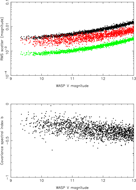
Figure 2: Upper panel: RMS scatter versus magnitude prior to decorrelation with SysRem. The upper curve shows the RMS scatter of individual data points in the light-curves of the non-variable stars in the ensemble. The middle curve shows the scatter in the same light-curves after performing a moving weighted average over all complete 2.5-hour intervals within each night. The lower curve shows the RMS scatter of the individual data points divided by the square root of the average number of points (typically 22) in a 2.5-hour interval. The correlated noise amplitude among the brightest stars is typically 0.0025 mag. Lower panel: Covariance spectral index $b$ as a function of $V$ magnitude prior to decorrelation with SysRem. Pure uncorrelated (white) noise should give $b=-0.5$, while pure correlated noise should give $b=0$. We see that the effects of correlated noise are most pronounced for the brightest stars. Even the faintest stars are affected to some extent.

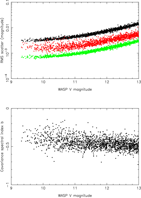
Figure 3: Upper panel: RMS scatter versus magnitude after removal of the four strongest correlated error components using SysRem. The curves are defined as in Fig. 2. The correlated noise amplitude of the binned data is reduced to 0.0015 magnitudes for the brightest stars. Lower panel: Covariance spectral index $b$ as a function of $V$ magnitude after removal of 4 correlated error components using SysRem. While some effects of correlated noise remain for the brightest stars, stars fainter than $V=11.0$ have covariance spectral indices close to the value $b=-0.5$ expected for white noise.

These systematic errors, and no doubt others as-yet unidentified, have a serious impact on the detection threshold for transits. Pont (2006) discussed methods of characterising the structure of the covariance matrix for a given stellar light-curve. The first and simplest method is to carry out boxcar smoothing of each night’s data, with a smoothing length comparable to the typical 2.5-hour duration of a planetary transit. For every set of $L$ points spanning a complete 2.5-hour interval interval starting at the $k$th observation, we construct an optimally-weighted average magnitude

$$\hat{m}_{k}=\frac{\sum_{i=k}^{k+L-1}m_{i}w_{i}}{\sum_{i=k}^{k+L-1}w_{i}},$$

with bad observations down-weighted as above using $w_{i}=1/(\sigma^{2}_{i}+\sigma^{2}_{t(i)})$.

The RMS scatter $\sigma_{\mbox{binned}}$ in the smoothed light-curve of $\hat{m}_{k}$ values is then compared to the RMS scatter $\sigma_{\mbox{unbinned}}$ of the individual data points. For uncorrelated noise, we expect $\sigma_{\mbox{binned}}=\sigma_{\mbox{unbinned}}/\sqrt{L}$, where $L$ is the average number of observations made in a 2.5-hour interval. In Fig. 2 we plot $\sigma_{\mbox{unbinned}}$, $\sigma_{\mbox{binned}}$ and $\sigma_{\mbox{unbinned}}/\sqrt{L}$ as functions of $V$ magnitude. For clarity, we exclude all obviously variable stars having $\sqrt{\sigma^{2}_{s(j)}}>0.005$ magnitude (as defined in Eq. 4). The RMS scatter in the binned data is typically 0.0025 magnitude for the brightest non-variable stars, far worse than the 0.0008 magnitude that would be achieved if the noise were uncorrelated.

The covariance structure of the correlated noise is quantified by the power-law dependence of the RMS scatter on the number of observations used in the boxcar smoothing:

$$\sigma_{\mbox{binned}}=\sigma_{\mbox{unbinned}}L^{b}.$$

For completely uncorrelated noise we expect $b=-1/2$, while for completely correlated noise (e.g. from intrinsic large-amplitude stellar variability on timescales longer than the longest smoothing length considered but shorter than the data duration) we expect the RMS scatter to be independent of the number of data points, giving $b=0$. We measure $b$ for each star using the incomplete smoothing intervals at the start and end of the night. We create a set of binned magnitudes obtained for $L=1,2,3,...$ consecutive observations. The RMS scatter in the binned magnitudes for each value of $N$ is then plotted as a function of $L$ and a power-law fitted to determine $b$. In Fig. 2 we plot $b$ as a function of $V$ magnitude, again excluding intrinsic variable stars having $\sqrt{\sigma^{2}_{s(j)}}>0.005$ magnitude. As expected, we find the effects of correlated noise to be most pronounced for the brightest non-variable stars. Even at our faint cutoff limit of $V=13$, however, we do not fully recover the uncorrelated noise value $b=-0.5$.

We use the SysRem algorithm of Tamuz et al. (2005) to identify and remove patterns of correlated noise in the data. The reader is referred to that paper for details of the implementation. The SysRem algorithm produces a corrected magnitude $\tilde{x}_{i,j}$ for star $j$ at time $i$, given by

$$\tilde{x}_{i,j}=x_{i,j}-\sum_{k=1}^{M}\ {}^{(k)}c_{j}\ ^{(k)}a_{i}.$$

where $M$ represents the number of basis functions (each representing a distinct pattern of systematic error) removed. An interesting property of the SysRem algorithm is that the inverse variance weighted mean value of each basis function, multiplied by the corresponding stellar coefficient, is so close to zero for all but the most highly variable stars that it is not necessary to repeat the coarse decorrelation. The inverse variance weighted mean change in the zero-point of each frame is generally less than 0.001 magnitude, again rendering further coarse decorrelation unnecessary after the final application of SysRem.

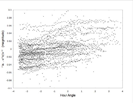
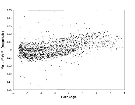
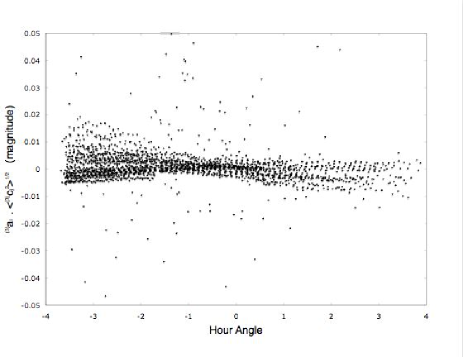
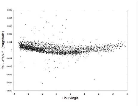
Figure 4: The first four SysRem basis functions are plotted as a function of hour angle after being folded on a period of 1 sidereal day. To give an idea of the magnitude correction applied to a typical star, each basis function is scaled by the RMS scatter of the corresponding stellar coefficients.

As described by Tamuz et al, we find several distinct basis functions $a_{i}$ representing patterns of correlated systematic error in the data which affect every star in the field to an extent quantified by the coefficents $c_{j}$. In Fig. 4 we plot the first four basis functions against hour angle, after folding the entire season’s basis-function values on a period of 1 sidereal day. The first and strongest basis function produced by SysRem shows a generally smooth night-to-night variation ${}^{(1)}a_{i}$ with a characteristic timescale of order 10 days. Superimposed on this large-amplitude, long-timescale variation is a small-amplitude, linear trend through each night. Neither variation appears to be related directly to either the lunar cycle or to transparency losses caused by intermittent Sahara dust events, but the stellar coefficients ${}^{(1)}c_{j}$ show a strong correlation with magnitude at $V>12$. We infer that this systematic error component may be related to a combination of sky brightness and atmospheric transparency that could affect the rejection threshold for faint stellar images in the sky aperture, leading the pipeline to underestimate the brightness of faint stars in bright moonlight and/or poor transparency.

The second and fourth basis functions resemble half-sinusoids, 90 degrees out of phase, when plotted modulo sidereal time. Both the secondary extinction and the flat-field vignetting correction are expected to vary as functions of sidereal time. As discussed above, SuperWASP is not autoguided, and a small misalignment of the polar axis causes stellar images to re-trace the same path across the CCD, a few tens of pixels long, every sidereal day. The second and fourth basis functions are probably a linear combination of these two effects. The corresponding stellar coefficients ${}^{(2)}c_{j}$ and ${}^{(4)}c_{j}$ should be correlated with departures from the stellar colour used for the extinction modelling, and with the gradient of the residuals in the vignetting function along the trajectory of each stellar image. The third basis function is a linear trend through the night, generally increasing but occasionally decreasing. The origin of this component is not obvious, but one possibility is that it could arise from temperature-dependent changes in the camera focus through the night.

The fifth and higher basis functions gave significantly smaller changes in $\chi^{2}$ than the first four, and their form appears to represent mainly stochastic events affecting only a few points in the light-curves of a relatively small number of stars. To avoid the danger of removing genuine stellar variability, we modelled the global systematic errors using only the first four SysRem basis functions.

In Fig. 3 we show the RMS-magnitude diagram and covariance index $b$ as functions of $V$ magnitude after processing with SysRem. We find that for stars fainter then $V=11.0$ the noise in the corrected light-curves is almost uncorrelated. For brighter stars some residual evidence of correlated noise remains. On the 2.5-hour timescale of a typical transit, however, the RMS amplitude of the correlated noise component is reduced to values of order 0.0015 magnitude with the help of SysRem.

5 Hybrid transit-search algorithms

We use an adaptation of the BLS algorithm (Kovács et al., 2002) for the initial search. We set up a coarse search grid of frequencies and transit epochs. The frequency step is such that the accumulated phase difference between successive frequencies over the full duration of the dataset corresponds to the expected width of a transit at the longest period searched. A set of transit epochs is defined at each frequency, at phase intervals equal to the expected transit width at that frequency. The expected transit duration is computed from the orbital frequency using Kepler’s third law assuming a stellar mass of 0.9 M_⊙. Since the majority of the main-sequence stars in the magnitude range of interest have masses between 0.7 and 1.3 M_⊙ and the transit duration at a given period scales as $(M_{*}/M_{\odot})^{2/3}$, the predicted transit duration is unlikely to be in error by more than 20 to 30 percent even at the extremes of the mass range.

At each trial period and epoch, The transit depth and goodness-of-fit statistic $\chi^{2}$ are calculated using a variant of the optimal fitting methods of Kovacs et al, reformulated such that the goodness-of-fit criterion has the dimensions of the $\chi^{2}$ statistic. A similar approach has also been used by Aigrain & Irwin (2004) and by Burke et al. (2005).

After processing with SysRem, the light-curve of a given star comprises a set of observations $\tilde{x}_{i}$ with associated formal variance estimates $\sigma^{2}_{i}$ and additional, independent variances $\sigma^{2}_{t(i)}$ to account for transient spatial irregularities in atmospheric extinction. We define inverse-variance weights

$$w_{i}=\frac{1}{\sigma^{2}_{i}+\sigma^{2}_{t(i)}+\sigma^{2}_{s(j)}},$$

and subtract the optimal average value

$$\hat{x}=\frac{\sum_{i}\tilde{x}_{i}w_{i}}{\sum_{i}w_{i}}$$

to obtain $x_{i}=\tilde{x}_{i}-\hat{x}$. We also define

$$t=\sum_{i}w_{i},\hskip 5.69054pt\chi^{2}_{0}=\sum_{i}x_{i}^{2}w_{i},$$

summing over the full dataset. Note that the weights defined here include the independent variance component $\sigma^{2}_{s(j)}$. This has the effect of lowering the significance of high-amplitude variable stars, but has little effect on low-amplitude variables such as planetary transit candidates.

In the BLS method, the transit model is characterised by a periodic box function whose period, phase and duration determine the subset $\ell$ of “low” points observed while transits are in progress. In many implementations the partitioning of the data can be the slowest part of the BLS procedure (Aigrain & Irwin, 2004). We achieve substantial speed gains by computing the orbital phase $\phi$ of each data point and sorting the phases in ascending order together with their original sequence numbers. We partition the phase-ordered data into a contiguous block of out-of-transit points for which $w/2P<\phi<1-w/2P$, where $w$ is the transit duration and $P$ is the orbital period, and the complement of this subset comprising the in-transit points. The summations that follow use the phase-ordered array of sequence numbers to access the in-transit points.

Using notation similar to that of Kovács et al. (2002), we define

$$s=\sum_{i\in\ell}x_{i}w_{i},\hskip 5.69054ptr=\sum_{i\in\ell}w_{i},\hskip 5.69054ptq=\sum_{i\in\ell}x_{i}^{2}w_{i}.$$

The mean light levels inside ($L$) and outside($H$) transit are given by

$$L=\frac{s}{r},H=\frac{-s}{t-r}$$

with associated variances

$$\mbox{Var}(L)=\frac{1}{r},\hskip 5.69054pt\mbox{Var}(H)=\frac{1}{t-r}.$$

The fitted transit depth and its associated variance are

$$\delta=L-H=\frac{st}{r(t-r)},\hskip 5.69054pt\mbox{Var}(\delta)=\frac{t}{r(t-r)},$$

so the signal-to-noise ratio of the transit depth is

$$\mbox{S/N}=s\sqrt{\frac{t}{r(t-r)}}.$$

The improved fit to the data is given by $\chi^{2}=\chi^{2}_{0}-\Delta\chi^{2}$, where the improvement in the fit when compared with that of a constant light curve is

$$\Delta\chi^{2}=\frac{s^{2}t}{r(t-r)}.$$

Note also that $\Delta\chi^{2}=s\delta=(S/N)^{2}$. The goodness of fit to the portions of the light-curve outside transit, where the light level should be constant, is

$$\chi^{2}_{h}=\chi^{2}_{0}-\frac{s^{2}}{(t-r)}-q.$$

The best-fitting model at each frequency is selected, and the corresponding transit depth, $\Delta\chi^{2}$ and $\chi^{2}_{h}$ are stored for each star.

5.1 Selection of potential candidates

Following an initial, coarse application of the BLS algorithm, we filter the candidates by rejecting obviously variable stars for which the post-fit $\chi^{2}>3.5N$, where N is the number of observations. We reject stars for which the best solution has fewer than two transits. We also reject those best-fit solutions for which the phase-folded light curve contains gaps greater than 2.5 times the expected transit duration. Such solutions arise in a small number of stars that suffer from errors in the vignetting correction near the extremities of the field of view, or from transient dust motes in the optics that are not completely flat-fielded out. Stellar images drift across the image by a few dozen pixels during a typical night, because SuperWASP is unguided and has a small misalignment of the polar axis. The drift pattern in the light curve recurs on a period of one sidereal day and its form depends strongly on location. It is significant mainly around the edges of the chip and near transient dust-ring features in the flat field. The SysRem algorithm is not effective at removing this type of variation from the small number of stars affected, so we reject them at this stage in the analysis. There is sufficient overlap between cameras that there is a high probability of the same star being recorded in a less problematic part of an adjacent camera’s field of view.

We select candidates for finer analysis by making cuts on two light-curve statistics, in both of which we expect stars showing periodic transit signals to lie well out in one tail of the distribution. The first is the “signal-to-red noise” ratio $S_{\mbox{red}}$ of the best-fit transit depth to the RMS scatter binned on the expected transit duration:

$$S_{\mbox{red}}=\frac{\delta\sqrt{N_{t}}}{\sigma L^{b}}.$$

As in Sect. 4.2 above, $L$ is the average number of data points spanning a single transit, $b$ is the power-law index that quantifies the covariance structure of the correlated noise, $N_{t}$ is the number of transits observed, $\delta$ is the transit depth and $\sigma$ is the weighted RMS scatter of the unbinned data. Since the transit depth $\delta$ is a signed quantity, this statistic distinguishes periodic dimmings from periodic brightenings. The second statistic is the “anti-transit ratio” $\Delta\chi^{2}/\Delta\chi^{2}_{-}$ proposed by Burke et al. (2005), being the ratio of the strongest peak in the periodogram of $\delta\chi^{2}$ that corresponds to a dimming, to the strongest peak corresponding to a brightening. We adopt conservative thresholds, requiring $S_{\mbox{red}}<-5$ and $\Delta\chi^{2}/\Delta\chi^{2}_{-}>1.5$. Note that Burke et al use a threshold of 2.75 for final selection on the latter statistic.

Even this relatively loose set of selection criteria eliminates 95.5 to 97.5 percent of all the stars in the sample, typically leaving 100 to 200 surviving objects worthy of more detailed study from an initial sample of several thousand stars.

In order to ensure that the most obvious transit candidates are not rejected by the filtering, we injected synthetic patterns of transits, with randomly-generated periods and epochs, into the light-curves of 100 randomly-chosen stars in the test dataset. The transits were given depths of 0.02 magnitude, and their durations were again computed from the orbital frequency using Kepler’s third law assuming a stellar mass of 0.9 M_⊙. The synthetic transit signatures were added to the actual data, thus preserving the noise properties of the observations.

In Fig. 5 we plot the anti-transit ratio against $S_{\mbox{red}}$ for all stars in the dataset with positive values of $S_{\mbox{red}}$. The 100 stars for which synthetic transits were injected are denoted by crosses, and the remainder by dots. Those stars selected for further study are circled, confirming that the preselection procedure captures a set of objects that includes nearly all candidates with significant transit signals. Those that were not selected were either too faint and noisy to yield a significant detection, or were superimposed on light-curves of intrinsically variable stars that failed to satisfy the other selection criteria.

Figure 5: A scatterplot of the anti-transit ratio against the signal to red noise ratio for stars in the 0143+3126 field shows that the majority of non-variable stars yield anti-transit ratios less than 2.0, and spurious best-fit signal to red noise ratios between -3.0 and -6.0. Crosses denote the 100 stars for which synthetic transits with depths of 0.02 magnitude were injected. Stars that satisfy the initial selection criteria for refined analysis are circled.

5.2 Refinement of transit parameters

The reduced sample is again subjected to a BLS search, this time utilising a finer grid spacing in which the frequency step is chosen to give a phase drift over the entire data train that is no more than half the expected transit width. The grid spacing in epoch is set at half the transit width. For each star in the sample we identify the five most significant peaks that correspond to transit-like dimmings, and the three most significant peaks that correspond to brightenings. (Selecting the three most significant peaks at the resolution of the grid search suffices to capture the strongest peak reliably after Newton-Raphson refinement, but for dimmings we are interested in possible aliases, so we examine the five most significant peaks).

Having identified a subset of objects in which statistically-significant transit-like signals may be present, we next refine the transit parameters. Instead of using a pure box function we adopt a softened box-like function $\mu(t_{i})$ developed by Protopapas et al. (2005):

$$\mu(t_{i})=\frac{1}{2}\delta\left(\tanh\left[c(t_{p}+\frac{1}{2})\right]+\tanh\left[c(t_{p}-\frac{1}{2})\right]\right)$$

to approximate the light-curve at time $t_{i}$, where

$$t_{p}=\frac{P\sin[\pi(t-T_{0})/P]}{\pi\eta}.$$

Here $T_{0}$ is the epoch of mid-transit, $P$ is the orbital period, $\delta$ is the transit depth, $\eta$ is the transit duration and $c$ is a softening parameter that determines the duration of ingress and egress in the model transit.

This function has the advantage that it is analytically differentiable with respect to the key transit parameters $T_{0}$, $P$, $w$ and $\delta$, which means that we can refine them quickly and efficiently using a Newton-Raphson approach based on the derivative functions $d\mu/dT_{0}$, $d\mu/dP$ and $d\mu/d\eta$.

For an estimated set of parameters $T_{0}$, $P$, $\eta$ we fit the transit depth by defining a basis function

$$p_{i}=d\mu(t_{i})/d\delta=\mu(t_{i})/\delta$$

and, for each observation $x_{i}$, determine the optimal scaling factor to fit the light-curve:

$$\hat{\delta}=\frac{\sum_{i}(x_{i}-\hat{x})(p_{i}-\hat{p})w_{i}}{\sum_{i}(p_{i}-\hat{p})^{2}w_{i}}$$ (7)

where $\hat{x}=\sum_{i}x_{i}w_{i}/\sum_{i}w_{i}$ and $\hat{p}=\sum_{i}p_{i}w_{i}/\sum_{i}w_{i}$.

At this stage in the analysis we omit the variance component $\sigma^{2}_{s(j)}$ due to stellar variability, but retain the patchy-extinction contribution $\sigma^{2}_{t(i)}$ so that poor quality data are down-weighted correctly:

$$w_{i}=\frac{1}{\sigma^{2}_{i}+\sigma^{2}_{t(i)}}.$$

We refine the model parameters $T_{0}$, $P$ and $\eta$ in turn. To refine the epoch of transit, for instance, we subtract the current model from the data to obtain

$$y_{i}=x_{i}-\mu(t_{i}),$$

and define the basis function

$$q_{i}=d\mu(t_{i})/dT_{0}.$$

We then determine the optimal scaling factor

$$\hat{dT}_{0}=\frac{\sum_{i}(y_{i}-\hat{y})(q_{i}-\hat{q})w_{i}}{\sum_{i}(q_{i}-\hat{q})^{2}w_{i}}$$ (8)

where $\hat{y}=\sum_{i}y_{i}w_{i}/\sum_{i}w_{i}$ and $\hat{q}=\sum_{i}q_{i}w_{i}/\sum_{i}w_{i}$.

The new estimate of the transit epoch is $T_{0}+dT_{0}$, so we re-compute $\mu$ and redetermine the transit depth using Eq. 7. The period $P$ and transit width $\eta$ are refined in turn using procedures exactly analogous to Eq. 8. The parameter values converge rapidly to the optimal solution after a few iterations.

At this stage the phased light-curves of the best-fit solutions are inspected visually to pick out those candidates showing clear transit-like signatures. Candidates identified in this way from the 0143+3126 field are listed in Table 1, and a representative selection of their phased light-curves are shown in Fig. 6. Some of these are clearly eclipsing binaries, exhibiting secondary eclipses, out-of-transit variability, or both. Further physical characterisation is needed to distinguish plausible planetary transit candidates from probable stellar impostors.

Figure 6: Representative light curves and periodograms of four objects in the 0143+3126 field exhibiting transit-like behaviour. The fourth object, 1SWASP J014228.76+335433.9, shows clear ellipsoidal variability outside transit, indicating a stellar binary.

Figure 7: continued

6 Characterization of candidates

Both theory (Brown, 2003) and the experience of previous transit follow-up campaigns (Alonso et al. 2004; Bouchy et al. 2005; Pont et al. 2005; O’Donovan et al. 2006) indicate that among our transit candidates, stellar binaries will outnumber genuine planetary transits by an order of magnitude. Some are grazing eclipsing binaries; others are multiple systems in which the light of a stellar eclipsing pair is diluted; others still have low-mass stellar or brown-dwarf companions whose radii are similar to those of gas-giant planets. In order to mitigate the false-alarm rate our candidates must pass a number of tests before being considered as high-priority spectroscopic targets.

6.1 Ellipsoidal variations

Drake (2003) and Sirko & Paczyński (2003) pointed out that ellipsoidal variables can be rejected with a high degree of certainty as stellar binaries. Detached stellar binaries with orbital periods of 1 to 5 days can easily be mistaken for transiting exoplanet systems if they exhibit either grazing eclipses or deeper eclipses diluted by the light of a blended third star. In either case, the equipotential surfaces of the two stars will often be sufficiently ellipsoidal to yield detectable out-of-transit variability.

Since the data have already been partitioned into a subsets of points inside and outside transit, we approximate the ellipsoidal variation with phase angle $\theta_{i}$ as

$$p_{i}=-\cos 2\theta_{i}$$

to the out-of-transit residuals $x_{i}-H$. We sum over the subset $h$ of points outside transit to define

$$u=\sum_{h}(x_{i}-H)p_{i}w_{i},\hskip 28.45274ptv=\sum_{h}p_{i}^{2}w_{i}$$

and so obtain both the amplitude and formal variance

$$\epsilon=\frac{u}{v},\hskip 28.45274pt\mbox{Var}(\epsilon)=\frac{1}{v}$$

of the ellipsoidal variation. The signal-to-noise ratio of the amplitude is

$$\mbox{S/N}=\sqrt{\Delta\chi^{2}_{\epsilon}}=\frac{u}{\sqrt{v}}.$$

Any candidate for which the sign of $\epsilon$ indicates that the system is significantly brighter at quadrature than at conjunction, with S/N$>5$ or so, is noted as a probable stellar impostor. In Table 1 we see that two of the possible transit-like candidates identified by eye are disqualified in this way.

The 5$\sigma$ detection threshold for ellipsoidal variation is nearly independent of orbital period, but ranges from to 0.003 magnitude at $V=12.5$ to 0.001 mag at $V=10$ for the dataset studied here. The expected amplitude of ellipsoidal variation depends on the ratio of the primary radius to the orbital separation, and on the mass ratio of the system.

The SuperWASP transit search yields many objects in which a solar-type star appears in a 1 to 2-day orbit about a companion with a radius of 1 to 2 R${}_{\mbox{Jup}}$. Simple projected-area calculations based on a standard Roche equipotential surface model for a main-sequence star of 1 M_⊙ with a 0.2 M_⊙ companion in a 1.5-day orbit yield an ellipsoidal variation of order 0.002 magnitude, which should be detectable with high significance in an isolated system with $V<11$ or so. Companions less massive than this may not yield detectable ellipsoidal variations, but are sufficiently interesting in their own right to be worth following up.

Ellipsoidal variability can also help to eliminate impostor systems where a bright foreground star is blended with a background eclipsing binary. If one component of an eclipsing stellar binary is evolved, such as in an RS CVn system with a 2.5 to 3.0 R_⊙ K subgiant and a solar-type main-sequence star in a 3-day orbit, the ellipsoidal variation can be as great as 0.02 to 0.05 magnitude. If such a system exhibits a partial primary eclipse 0.1 to 0.3 magnitude deep and a shallow secondary eclipse, and is blended with a foreground star 2 to 3 magnitudes brighter, it can mimic an exoplanetary transit. The ellipsoidal variation is thus great enough to remain detectable even when diluted by a blend 2 or 3 magnitudes brighter.

Table 1: Transit candidates identified by eye from 0143+3126 field. Quantities that disqualify a candidate from further consideration are shown in boldface. IDs of disqualified candidates are shown in parentheses.

SuperWASP ID	$S_{\mbox{red}}$	$\delta$	Duration (h)	Epoch	Period	$N_{t}$	$(S/N)_{\mbox{e}llip}$
(1SWASP J015721.21+333517.9)	27.4	0.0518	1.704	3182.1328	4.14907	2	2.1
1SWASP J013901.75+333640.6	21.2	0.1781	2.04	3180.9563	3.440225	5	3.6
1SWASP J015711.29+303447.7	12.3	0.0155	2.304	3182.5613	2.042603	9	1.3
(1SWASP J014228.76+335433.9)	13.4	0.0385	3.648	3180.7258	2.02348	12	16.5
1SWASP J014400.22+344449.2	11.9	0.0273	3.168	3180.2839	3.719753	5	4.4
1SWASP J015625.53+291432.5	12.2	0.0124	3.216	3182.5415	1.451347	13	4.9
1SWASP J014212.56+341534.4	11.3	0.0632	2.904	3182.0596	4.305729	6	4.7
1SWASP J014211.84+341606.5	11.1	0.0544	3.072	3182.0503	4.30604	6	4.2
(1SWASP J012536.11+341423.8)	8.9	0.0623	2.52	3181.6191	1.891481	4	9.5
1SWASP J014549.24+350541.9	6.9	0.0081	2.256	3182.407	1.452465	9	0.6
1SWASP J014700.48+280243.6	6.7	0.008	4.32	3182.1853	1.68013	13	0.5

6.2 Stellar mass and planet radius

Seager & Mallén-Ornelas (2003) and Tingley & Sackett (2005) have developed methods for deriving the physical parameters of transit candidates based on light-curve parameters alone. Seager & Mallen-Ornelas use the orbital period, the total transit duration, the duration of ingress and egress and the transit depth to derive the impact parameter, the orbital inclination, the stellar mass, the planet radius and the orbital separation. Because the duration of ingress and egress are difficult to measure reliably in noisy data, we define a simplified consistency test predicated on the assumption that the orbital inclination is close to 90 degrees. Our aim is simply to estimate the mass of the star and the radius of the planet, and thereby to determine whether the transits could plausibly be caused by a roughly Jupiter-sized planet orbiting a star of roughly solar mass and radius.

Once an object is found to display transit-like events (characterised by a flat light-curve outside eclipse, no secondary eclipse and a transit depth $<0.1$ mag) we search the USNO-B1.0 catalogue for blends less than 5 mag fainter, located within the 48-arcsec radius of the 3.5-pixel photometric aperture. We estimate a main-sequence radius and mass from a $V-K$ colour index derived from the SuperWASP $V$ magnitude and the 2MASS $K$ magnitude. We infer both the expected transit duration and the radius of the putative planet using the simplified mass-radius relation of Tingley & Sackett (2005),

$$R_{\star}\simeq M_{\star}^{4/5}.$$

The size of the planet follows from the approximate expression of Tingley & Sackett (2005) for the transit depth $\delta$ for a limb-darkened star:

$$\frac{R_{p}}{R_{\star}}\simeq\sqrt{\frac{\delta}{1.3}}.$$

High-priority candidates must display multiple transits, a fitted transit duration no more than 1.5 times more or less than the predicted value, a transit depth indicating a planetary radius less than 1.6 Jupiter radii, and have no blends less than 3 magnitudes fainter located within the 48 arcsec photometric aperture. Their proper motions (from the Hipparcos, tycho-2 or USNO-B1.0 catalogues) and $V-K$ colours must also be consistent with main-sequence stars rather than giants, the luminosity class being inferred from the reduced proper-motion method of Gould & Morgan (2003) and the giant-dwarf separation method of Bilir et al. (2006).

In Table  2 we list the effective temperatures, spectral types and stellar radii estimated from the $V-K$ colour indices, together with the inferred planet radius and the ratio $\eta$ of the observed to the expected transit duration. The effective temperatures are derived using the calibration of Blackwell & Lynas-Gray (1994), and the radii using the interferometrically-determined colour-surface brightness relations of Kervella et al. (2004) together with Hipparcos parallaxes, where available. Two objects are rejected immediately, because brighter stars are found within the radius of the photometric aperture. Both stars found previously to exhibit significant ellipsoidal variations yield inferred companion radii 2.46 and 1.63 R${}_{\mbox{Jup}}$, substantially greater than expected for gas-giant planets. Four of the remaining candidates are rejected on the same grounds.

Of the original eleven candidates, three remain. 1SWASP J015625.53+291432.5 and 1SWASP J014549.24+350541.9 are mid-K stars, for which the inferred companion radii are substantially less than that of Jupiter. Both of these have stars less than 5 magnitudes fainter located within the photometric aperture, so further follow-up is warranted to eliminate the possibility that the blended stars could be eclipsing binaries. The transit detection in 1SWASP J014549.24+350541.9 is of rather marginal significance, with $S_{\mbox{red}}=6.93$. The brightest of the three candidates, 1SWASP J015711.29+303447.7, appears to be an F6 star with a 1.38 R${}_{\mbox{Jup}}$ companion.

Table 2: Estimated physical parameters for transit candidates in 0143+3126 field. Parameter values inconsistent with planetary status are highlighted in bold type. IDs of stars disqualified on these grounds are shown in parentheses.

SuperWASP ID	$V_{T}$(SW)	$V-K$	$T_{\rm eff}$	Sp. type	$R_{*}/R_{\odot}$	$R_{p}/R_{\mbox{J}up}$	$\eta$	$N_{\rm brighter}$	$N_{<5{\mbox{mag fainter}}}$
(1SWASP J015721.21+333517.9)	10.982	1.36	6118	F8	1.18	2.29	0.44	0	0
(1SWASP J013901.75+333640.6)	12.986	1.86	5498	G8	0.89	3.2	0.58	0	2
1SWASP J015711.29+303447.7	10.352	1.19	6354	F6	1.3	1.38	0.77	0	0
(1SWASP J014228.76+335433.9)	10.963	0.93	6740	F2	1.47	2.46	1.08	0	1
(1SWASP J014400.22+344449.2)	11.164	1.3	6200	F8	1.22	1.72	0.88	0	1
1SWASP J015625.53+291432.5	10.294	2.3	5044	K3	0.76	0.72	1.67	0	1
(1SWASP J014212.56+341534.4)	12.247	1.37	6105	F9	1.17	2.51	0.74	0	1
(1SWASP J014211.84+341606.5)	12.359	n/a	n/a	n/a	n/a	n/a	n/a	2	2
(1SWASP J012536.11+341423.8)	12.336	2.26	5081	K2	0.77	1.64	1.07	0	1
1SWASP J014549.24+350541.9	11.44	2.45	4908	K4	0.73	0.56	1.22	0	2
(1SWASP J014700.48+280243.6)	11.764	n/a	n/a	n/a	n/a	n/a	n/a	1	1

7 Discussion and conclusions

In this paper we have described the methodology that we have adopted for searching for transits in the large body of data produced by the SuperWASP camera array on La Palma during its first few months of operation, and applied it to the 7840 stars brighter than $V=13.0$ in a survey field centred at RA 01h 43m, Dec +31^∘ 26’.

We find that an initial search using the BLS method on a coarse grid of transit epochs and orbital frequencies is sufficient for us to eliminate more than 95 percent of the stars searched. This allows us to perform a finer grid search on only the remaining 198 stars in the field under consideration. We have adapted the analytic Newton-Raphson method of Protopapas et al. (2005) to refine the orbital solutions around periodogram peaks found with the BLS method. This method quickly yields the depth and duration of the transits, and the frequency and phase of the photometric orbit, while keeping the dimensionality of the search grid (and hence the processing time required) as low as possible.

We use the ellipsoidal-variation methodology of Drake (2003) and Sirko & Paczyński (2003) in our light-curve modelling to eliminate probable stellar binaries. We use the publicly-available 2MASS and USNO-B1.0 catalogues to obtain colours and proper motions for candidates, and to estimate the stellar and planetary radii using methods similar to those of Seager & Mallén-Ornelas (2003) and Tingley & Sackett (2005). These methods confirm that two of our most significant transit detections in this field, and one more marginal one, have transit properties fully consistent with those expected for planets with radii comparable to or somewhat smaller than Jupiter.

The survey field chosen to illustrate the method is only one of more than 100 such regions surveyed during the course of 2004. Candidates from the other fields will be presented and discussed in subsequent papers. Together with the three candidates presented here, all likely planetary-transit candidates will be subjected to high-resolution spectroscopic follow-up in the latter half of 2006, using the methodology employed successfully by Bouchy et al. (2005) for OGLE-III follow-up.

References

- Aigrain & Irwin (2004) Aigrain S., Irwin M., 2004, MNRAS, 350, 331
- Alonso et al. (2004) Alonso R., Brown T. M., Torres G., Latham D. W., Sozzetti A., Mandushev G., Belmonte J. A., Charbonneau D., Deeg H. J., Dunham E. W., O’Donovan F. T., Stefanik R. P., 2004, ApJ, 613, L153
- Bertin & Arnouts (1996) Bertin E., Arnouts S., 1996, A&AS, 117, 393
- Bilir et al. (2006) Bilir S., Karaali S., Güver T., Karataş Y., Ak S. G., 2006, Astronomische Nachrichten, 327, 72
- Blackwell & Lynas-Gray (1994) Blackwell D. E., Lynas-Gray A. E., 1994, A&A, 282, 899
- Bouchy et al. (2005) Bouchy F., Pont F., Melo C., Santos N. C., Mayor M., Queloz D., Udry S., 2005, A&A, 431, 1105
- Brown (2003) Brown T. M., 2003, ApJ, 593, L125
- Burke et al. (2005) Burke C. J., Gaudi B. S., DePoy D. L., Pogge R. W., 2005, ArXiv Astrophysics e-prints
- Charbonneau et al. (2005) Charbonneau D., Allen L. E., Megeath S. T., Torres G., Alonso R., Brown T. M., Gilliland R. L., Latham D. W., Mandushev G., O’Donovan F. T., Sozzetti A., 2005, ApJ, 626, 523
- Charbonneau et al. (2000) Charbonneau D., Brown T. M., Latham D. W., Mayor M., 2000, ApJ, 529, L45
- Deming et al. (2006) Deming D., Harrington J., Seager S., Richardson L. J., 2006, ApJ, 644, 560
- Deming et al. (2005) Deming D., Seager S., Richardson L. J., Harrington J., 2005, Nature, 434, 740
- Drake (2003) Drake A. J., 2003, ApJ, 589, 1020
- Gould & Morgan (2003) Gould A., Morgan C. W., 2003, ApJ, 585, 1056
- Høg et al. (2000) Høg E., Fabricius C., Makarov V. V., Bastian U., Schwekendiek P., Wicenec A., Urban S., Corbin T., Wycoff G., 2000, A&A, 357, 367
- Kervella et al. (2004) Kervella P., Thévenin F., Di Folco E., Ségransan D., 2004, A&A, 426, 297
- Kovács et al. (2002) Kovács G., Zucker S., Mazeh T., 2002, A&A, 391, 369
- Mazeh et al. (2005) Mazeh T., Zucker S., Pont F., 2005, MNRAS, 356, 955
- Monet et al. (2003) Monet D. G., Levine S. E., Canzian B., Ables H. D., Bird A. R., Dahn C. C., Guetter H. H., Harris H. C., Henden A. A., Leggett S. K., Levison H. F., Luginbuhl C. B., Martini J., Monet A. K. B., Munn J. A., Pier J. R., Rhodes A. R., Riepe B., Sell S., Stone R. C., Vrba F. J., Walker R. L., Westerhout G., Brucato R. J., Reid I. N., Schoening W., Hartley M., Read M. A., Tritton S. B., 2003, AJ, 125, 984
- O’Donovan et al. (2006) O’Donovan F. T., Charbonneau D., Torres G., Mandushev G., Dunham E. W., Latham D. W., Alonso R., Brown T. M., Esquerdo G. A., Everett M. E., Creevey O. L., 2006, ApJ, 644, 1237
- Pollacco et al. (2006) Pollacco D., Skillen I., Collier Cameron A., Christian D., Hellier C., Irwin J., Lister T., Street R., West R., Anderson D., Clarkson W., Deeg H., Evans A., Fitzsimmons A., Haswell C., Hodgkin S., Horne K., Jones B., Kane S., Keenan F., Maxted P., Norton A., Osborne J., Ryans R., Smalley B., Wheatley P., Wilson D., 2006, PASP, Submitted
- Pont (2006) Pont F., 2006, in Arnold L., Bouchy F., Moutou C., eds, Tenth Anniversary of 51 Peg-b: Status of and prospects for hot Jupiter studies Photometric searches for transiting planets: results and challenges. pp 153–164
- Pont et al. (2005) Pont F., Bouchy F., Melo C., Santos N. C., Mayor M., Queloz D., Udry S., 2005, A&A, 438, 1123
- Protopapas et al. (2005) Protopapas P., Jimenez R., Alcock C., 2005, MNRAS, 362, 460
- Sato et al. (2005) Sato B., Fischer D. A., Henry G. W., Laughlin G., Butler R. P., Marcy G. W., Vogt S. S., Bodenheimer P., Ida S., Toyota E., Wolf A., Valenti J. A., Boyd L. J., Johnson J. A., Wright J. T., Ammons M., Robinson S., Strader J., McCarthy C., Tah K. L., Minniti D., 2005, ApJ, 633, 465