Probing Dark Energy with Baryonic Acoustic Oscillations at High Redshifts

Abstract

Context. To constrain different cosmological models and especially the equation of state parameter $w$ of dark energy, the phases and amplitudes of baryonic acoustic oscillations in the galaxy power spectrum can be used as cosmological probes.

Aims. It will be shown that the phases as well as the amplitudes of baryonic acoustic oscillations can be extracted out of a galaxy power spectrum, including various observational effects like growth suppression, redshift space distortions, and galaxy biasing. The phases of baryonic acoustic oscillations are used as a standard ruler for a cosmological test to constrain $w$ over a large redshift range with a minimum of assumptions.

Methods. A non-oscillating phenomenological fitting function is used to extract the oscillatory part of the galaxy power spectrum and to disentangle phase information from amplitude information. The method (FITEX) is tested with simulated data of the Hubble Volume Simulation to include redshift space effects, non-linear structure growth and biasing. A cosmological test is introduced, which compares the extracted oscillations against a theoretical model template to derive constraints on the $w$ parameter.

Results. The phenomenological fitting function is found to model the various distortions of the galaxy power spectrum to the sub-percent level. The various distortions only boost the amplitude of the oscillations. The theoretical template is accurate enough to test for small deviations in the phases of the oscillations, resulting from different $w$ values. A cosmological test, using the baryonic acoustic oscillations as a standard ruler, is able to constrain $w$ in a robust way. These constraints are based solely on the phase of these oscillations, assuming no errors of the value at the end of the Compton drag epoch, as the standard ruler. The $w$ constraints are expected to further improve when the full two dimensional redshift space effects and the amplitudes of the baryonic acoustic oscillations are taken into account.

Conclusions.

1 Introduction

Acoustic oscillations as observed in the temperature anisotropies of the cosmic microwave background radiation (CMB) are traditionally used to constrain the values of certain cosmological parameters. The intrinsic amplitudes and locations of the oscillations are determined by the densities and pressures of the various energy components in the very early and hot Universe. The oscillations are furthermore modified by their subsequent geometric projection onto the present hypersphere, where they are observed. It turns out that both intrinsic CMB oscillations and their geometric projection are mainly shaped by the physical properties at high redshifts. Excluding the very large scales where cosmic variance makes analysis quite difficult, the observed oscillations in the CMB are highly degenerate against certain changes of the energy density $\rho_{\rm DE}$ and the equation of state parameter, $w=p_{\rm DE}/\rho_{\rm DE}c^{2}$, of the dark energy, dominating at low redshifts (see also Caldwell, Dave & Steinhardt 1998).

However, related so-called baryonic acoustic oscillations (BAOs) are expected to be observable at lower redshifts in the matter power spectrum. Therefore, the phases of the BAOs can be used as cosmic rulers in a similar manner as the CMB oscillations, but now at much smaller redshifts (Eisenstein, Hu & Tegmark 1998). Here, the observed phases are affected by the late-time geometry and thus by the value of $w$, the prime cosmological parameter of the present investigation.

The BAOs are classical Doppler peaks in the density distribution of matter (e.g. Hu & Sugiyama 1996). They are triggered in the hot Universe by oscillatory velocity patterns of the baryons. These velocity oscillations are generated, in the same environment as the CMB density oscillations, by sound waves on scales where radiation pressure could stabilize the fluid against gravitational collapse. At later times, this oscillatory velocity pattern of the baryon field produces kinematically a new field of matter density fluctuations in form of quasi-regular matter oscillations. The amplitudes of these BAOs are determined by the ratio of baryonic matter to the overall matter density. The BAOs thus constitute a quasi-regular pattern of oscillating substructures superposed with small amplitudes onto a general density field which fluctuates irregularly with several 100 times higher amplitudes.

The imprints of the BAOs on galaxy and clusters distributions, gravitational shear maps etc. can provide at least in principle a clean cosmic ruler for precise tests of the $w$ parameter. The characteristic scale, $s$, of these imprints is the comoving distance, sound waves can travel during the epoch where baryons and photons are strongly coupled through Compton and Thomson scattering (Compton drag). Cosmological tests based on the resulting sound horizon, $s$, as a metric ruler are expected to have only very small systematic errors because the phases of the BAOs located at scales small compared to $s$ are solely determined by well-understood physical processes. A practical problem is, however, to separate the oscillatory BAO modes from the irregular fluctuation field with sufficient accuracy.

One might object that the small amplitudes of the BAOs can easily be washed out especially by structure growth which can mix perturbation modes with adjacent wavenumbers $k$. This is certainly true for oscillations in the non-linear regime (Meiksin, White & Peacock 1999). On larger scales, however, recent observations of 2dF galaxies at redshifts $z<0.3$ clearly show several BAOs in the galaxy power spectrum (Cole et al. 2005). In addition, the sequence of BAOs in $k$-space is projected into a single wiggle in the space domain. The corresponding excess galaxy correlation was in fact observed in the two-point spatial correlation function of the luminous red SDSS galaxies at $z<0.5$ (Eisenstein et al. 2005). In addition to these observational indications, results from recent numerical simulations suggest that within certain redshift and scale ranges, stable BAOs could exist as useful probes for cosmological investigations (e.g. Seo & Eisenstein 2005, Springel et al. 2005, Jeong & Komatsu 2006). However, several critical issues like the exact behavior of baryons during structure growth on BAO-scales can only be discussed with much larger simulations and a better understanding of galaxy formation.

Applications of BAOs for cosmological tests of $w$ are confronted with the following situation. Present observational constraints of $w$ using different combinations of CMB, galaxy clusters, galaxies, and gravitational lensing data are all found to be consistent with $w=-1$, i.e., the value for the cosmological constant. The $1\sigma$ error of the $w$ values, derived from partially dependent observations, is around 10-20% (for a recent review see, e.g., Schuecker 2005). To improve current estimates, we thus have to extract the BAOs and to measure their phases quite accurately in the presence of non-linear and scale-dependent effects. Therefore, even tiny systematic errors in the analysis on percent levels can have severe consequences for the observational accuracy of $w$.

The basic aim of the present paper is to describe a new, simple, and robust method to extract BAOs from (non)linear, scale and redshift-dependent biased, redshift-space galaxy power spectra under realistic lightcone survey conditions. For brevity, we call the method ‘fit and extract’ (FITEX). The method has the potential to reduce many of the abovementioned sources of systematic errors. Our starting point is to use as few assumptions as possible for the extraction of the BAOs from a complex power spectrum. For reasons which will become clear later, we do the separation by fitting a flexible non-oscillating function to an observable which is directly related to the transfer function and not to the power spectrum itself. The crucial point is to show that BAOs extracted in this simple manner are still governed by simple physical processes, and that FITEX stays robust even under complex survey conditions. We believe that such model-independent approaches are quite important, especially in light of the fact that at least in the near future we cannot expect to model the abovementioned non-linear and scale-dependent effects with accuracies on the sub-percent level.

Our computations are in several cases optimized to galaxy surveys covering typically several 100 square degrees on the sky in the redshift range between $z=2-4$. This choice is motivated by the Hobby Eberly Dark Energy Experiment (HETDEX), which is planned to measure the $w$ parameter with several million Ly-$\alpha$ emitting galaxies at these redshifts (Hill & McQueen. 2004, Gebhardt et al. in prep.). We see the results of the present paper as a useful contribution to a realistic error forecast for this important project.

We organized the paper as follows. In Sect. 2 we motivate the basic idea of the FITEX algorithm. In the following sections we test its performance to separate BAOs from a complex power spectrum under linear conditions (Sect. 3), under quasi-non-linear conditions (Sect. 4), in redshift space (Sect. 5), and from biased samples (Sect. 6). Finally, we illustrate the performance of FITEX including all effects and use a cosmological test of $w$ as a benchmark to investigate the quality of the BAO extraction together with the theoretical template (Sect. 7). Our results are mainly based on a deep data wedge extracted by the Virgo Consortium from the Hubble Volume Simulation. The paper thus presents for the first time constraints on the application of BAOs for cosmological tests under realistic lightcone survey conditions.

If not mentioned explicitly, we assume a spatially flat Friedmann-Lemaître Robertson-Walker world model with the Hubble constant in units of $h=H_{0}/(100\,{\rm km}\,{\rm s}^{-1}\,{\rm Mpc^{-1}})$, the present values of the total matter density $\Omega_{\rm m}h^{2}=0.147$ and baryon density $\Omega_{\rm b}h^{2}=0.0196$, the density of relativistic matter (e.g. neutrinos) $\Omega_{\nu}=0$, and the mean CMB temperature $T_{\rm CMB}=2.728\,{\rm K}$ (concordance cosmology).

2 Baryonic Acoustic Oscillations (BAOs)

In this section, we discuss the ‘theoretical wiggle function’, that is, a reference function (see Eq. 1 below) we use in our cosmological tests of $w$ to match the BAOs extracted in a certain manner from the complex galaxy power spectrum. The power spectrum may be written in the form $P(k,z)\,=\,A(k,z,b)\,k^{n}\,T^{2}(k)$. The amplitude $A(k,z,b)$ includes the primordial amplitude, redshift and scale-dependent effects of redshift space distortions, linear and non-linear structure growth, and galaxy biasing which will be discussed in the course of the paper. The exponent $n$ is the slope of the primordial power spectrum, and $T(k)$ the transfer function. Our further treatment of the formation of BAOs is based on Hu & Sugiyama (1996) where a detailed description of the relevant physical processes can be found, and on the fitting equations derived by Eisenstein & Hu (1998).

Between the epoch of matter-radiation equality at redshift $z_{\rm eq}\approx 3526$ (concordance cosmology) and the end of the Compton drag epoch at $z_{\rm d}\approx 1026$, the baryons follow a regular velocity pattern which can generate new density fluctuations kinematically. On small scales and at $z_{\rm d}$, this effect (velocity overshoot) overrides the intrinsic density fluctuations of the baryons. As adiabatic modes dominate the isocurvature modes, the baryon density oscillates as $\sin(ks)$. The phase of the BAOs is frozen out at $z_{\rm d}$ at the value $ks$, with $s\approx 152\,{\rm Mpc}$ being the comoving sound horizon at $z_{\rm d}$ and $k$ the comoving wavenumber of the oscillation. The BAOs are thus $\pi/2$ out of phase with the corresponding CMB fluctuations. The sound horizon $s$ at $z_{\rm d}$ is the standard ruler we are looking for. Its value calibrates the phases of the theoretical wiggle function and can be measured quite easily with CMB experiments on the sub-percent level. This includes the contribution of unknown relativistic energy components (Eisenstein & White 2004). For consistency with the Hubble Volume Simulations (see Sect. 4) we use $\Omega_{\rm\nu}=0$.

The sinusoidal fluctuations in the baryon density are dampened by expansion drag, gravitational forcing, and Silk damping. In addition, cosmic expansion forces the velocity contributions to fall off at large scales, and amplitudes decline when dark matter dominates the energy density. While these effects only reduce the amplitude of the fluctuations and do not affect the phase, the damping may be summarized by the pseudo transfer function $T_{w}(k)\sim j_{0}(k\,s)e^{-(k/k_{\rm Silk})^{m_{s}}}/[1\,+\,(\beta_{b}\,/\,k\,s)^{3}]$, with $j_{0}$ the spherical Bessel function of order zero, the exponent $m_{\rm s}\,\approx\,1.4$ which is basically independent from cosmology, $k_{\rm Silk}=1.6(\Omega_{\rm b}h^{2})^{0.52}(\Omega_{\rm m}h^{2})^{0.73}[1+(10.4\Omega_{\rm m}h^{2})^{-0.95}]$, and $\beta_{b}=0.5+f_{\rm b}+(3-2f_{\rm b})\sqrt{(17.2\Omega_{\rm m}h^{2})^{2}+1}$ with $f_{\rm b}=\Omega_{\rm b}/\Omega_{\rm m}$. However, velocity overshoot dominates only on scales small compared to $s$. On larger scales, the original sound horizon, $s$, appears to be reduced by $(\tilde{s}/s)^{3}=1+(\beta/ks)^{3}$, with $\beta=8.41(\Omega_{\rm m}h^{2})^{0.435}$. This correction of $s$ is about 0.2% at $60\,h^{-1}\,{\rm Mpc}$ and 1.3% at $120\,h\,^{-1}\,{\rm Mpc}$. Though relatively small, the corrections are important as they change the length of the standard ruler $s$ depending on $k$. Collecting all scale-dependent terms we get the oscillatory solution (theoretical wiggle function)

$$T_{w}(k)\;\sim\;\frac{\,e^{-(k/k_{\rm Silk})^{m_{\rm s}}}}{1\,+\,(\beta_{b}\,/\,k\,s)^{3}}\,j_{0}(k\,\tilde{s})\,.$$ (1)

A way to extract BAOs from a complex power spectrum can be found when we specify the relation between the wiggle function, $T_{w}(k)$, and the total transfer function $T(k)$, which we discuss now. Each particle species, in the present case CDM and baryonic matter with the corresponding densities $\Omega_{\rm c}$ and $\Omega_{\rm b}$, should have separate effective transfer functions, $T_{c}$ and $T_{b}$. Though, after the drag epoch at $z_{\rm d}$, baryons appear basically pressureless and will fall into the potential wells of CDM. This results in a transfer function valid for both species of matter,

$$T(k)\,=\,\frac{\Omega_{\rm c}}{\Omega_{\rm m}}T_{c}(k)\,+\,\frac{\Omega_{\rm b}}{\Omega_{\rm m}}\,T_{b}(k)\,,$$ (2)

with $T_{c}(k)=f\tilde{T}_{0}(k,1,\beta_{c})+(1-f)\tilde{T}_{0}(k,\alpha_{c},\beta_{c})$, written in terms of the generalized transfer function $\tilde{T}_{0}(k,\alpha_{c},\beta_{c})$ as defined in Eisenstein & Hu (1998). Here, $f=1/[1+(ks/5.4)^{4}]$ smooths the combination of the almost baryon-free and baryon-loaded solutions near $s$, and

$$T_{b}(k)\,=\,\tilde{T}_{\rm b}(k)\,+\,T_{w}(k)\,,$$ (3)

where $\tilde{T}_{\rm b}(k)=\frac{j_{0}(k\tilde{s})\tilde{T}_{0}(k,1,1)}{1+(ks/5.2)^{2}}$. These approximations are better than 2% for $\Omega_{\rm b}\,/\,\Omega_{\rm m}\,<\,0.5$. Note that $\Omega_{\rm b}/\Omega_{\rm m}\rightarrow 0$ corresponds to $\alpha_{c},\beta_{c}\rightarrow 1$. If $\Omega_{\rm c}\,>>\,\Omega_{\rm b}$, the effects of dark matter dominate over velocity overshoot of the BAOs. Written in this way, we immediately see that the oscillatory part (1) is added on top of a non-oscillatory part and can be computed by subtracting off a smooth continuum from the complete transfer function. This process establishes the basic methodology of FITEX.

Figure 1: Comparison of different terms of the transfer function computed with $\Omega_{\rm b}\,h^{2}\,=\,0.0196$, $\Omega_{\rm m}\,h^{2}\,=\,0.147$ and $T_{\rm CMB}\,=\,2.728$ K. Upper panel: Non-oscillatory parts. The function $T_{\rm shape}$ is the sum of the other three. Lower panel: Oscillating parts. The residuals of the subtraction between the transfer function and its corresponding non-oscillatory fit is shown as long-dashed line. Note the different scaling of the y-axes. See main text for more details.

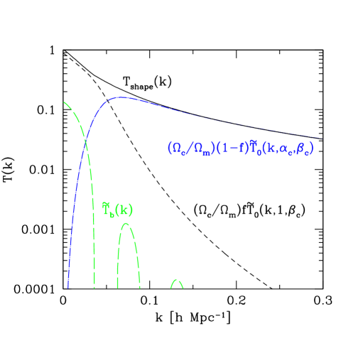
The different terms of the transfer function are shown in Fig. 1. The upper panel shows the components which determine the global shape of the transfer function. Note that an additional oscillating component, the first term in Eq. (3), is necessary to describe the transition from large to small scales with sufficient accuracy. This is a direct consequence of the fact that the main effect of the baryons on the transfer function is a damping of the overall growth of dark matter between $z_{\rm eq}$ and $z_{\rm d}$ which significantly reduces the fluctuation power at scales smaller than $s$. The resulting break is the imprint of the baryons on the power spectrum which is easiest to observe. The term $\tilde{T_{b}}$ thus contributes mainly to the shape as it is rapidly declining on scales smaller than $s$ to model the damping effect of the baryons.

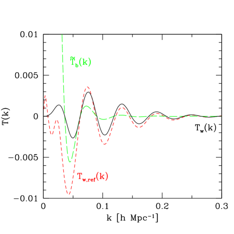
In the lower panel of Fig. 1, the two parts of the baryon transfer function are shown. One can clearly see the first to fifth oscillations. Note that $\tilde{T_{b}}$ declines very fast and is almost zero after the second oscillation. It is compared to the second term of the baryonic transfer function, $T_{w}(k)$, and a reference function, $T_{w,\textrm{ref}}$, which is formally constructed to contain all oscillations. Thus, the reference function includes both the small-scale oscillations from $T_{w}(k)$ and the large-scale oscillations from $\tilde{T}_{\rm b}(k)$. The latter is, however, also determined by the dark matter function $T_{0}(k,1,1)$ (see below Eq. 3). Therefore, excluding or including knowledge of the shape of the dark matter function for the extraction of BAOs corresponds to working either with $T_{w}(k)$ or with $T_{w,\textrm{ref}}$. Both $T_{w}(k)$ and $T_{w,\textrm{ref}}$ agree reasonably well beyond $k\,\geq\,0.05\,h\,\textrm{Mpc}^{-1}$, especially when one keeps in mind that only the phases of the oscillations are relevant as the amplitudes are subject to distortions anyway (see below).

The good agreement between the phases of $T_{w}(k)$ and $T_{w,\textrm{ref}}$ means, that quite simple physics as described by $T_{w}$ (mainly velocity overshoot and Silk damping) dominate the oscillations expected to be seen in the overall power spectrum. However, on larger scales, the physics get more complex due to the growing influence of CDM and the backreaction of the baryons on structure growth. Thus $T_{w}$ and $T_{w,\textrm{ref}}$ differ accordingly. Nevertheless, on small scales, $T_{w}$ is a good theoretical wiggle function for BAOs phases which can be used as a standard ruler for cosmological tests, with a minimum of theoretical assumptions.

3 Extracting BAOs under Linear Conditions

The main advantages of constraining cosmological parameters with BAOs are its small systematic errors, the ability to discriminate between geometrical effects (homogeneous universe) and structure growth effects (inhomogeneous universe) of cosmological parameters, and the potential to constrain dark energy without assuming a certain dark matter model. The observed phase of the BAOs is only affected by the geometry of the universe, while the observed amplitude of the oscillations is mainly affected by structure growth and other amplitude effects (see Sects. 4 to 6). It is thus very important to extract the BAOs from the power spectrum in a way that does not mix these two benchmarks. As suggested by the previous discussion, BAOs, described by simple physical processes, should be extracted by subtracting the shape of the non-oscillatory part of the transfer function. This method is able to disentangle phase effects from amplitude effects in an effective manner.

In contrast to this method, previous studies (Blake & Glazebrook 2003, Angulo et al. 2005, Hütsi 2005, Seo & Eisenstein 2005, White 2005) used the CDM-based theoretical non-oscillatory power spectrum, $P_{\rm ref}(k,z)$, given in Eisenstein & Hu (1998) to analyze the BAOs. This is done by dividing the measured power spectrum, $P_{\rm obs}(k,z)$, by this reference power spectrum. Assuming that the transfer function can be split into a shape part, $T_{\rm shape}$, and an oscillatory part, $T_{\rm wiggle}$, where $T_{\rm shape}\,>\,T_{\rm wiggle}$ (Sect. 2), the result of such a division is

$$\begin{split}\frac{P_{\rm obs}(k,z)}{P_{\rm ref}(k,z)}\;&=\;\frac{A_{\rm obs}(k,z)\,[T_{\rm shape}(k)\,+\,T_{\rm wiggle}(k)]^{2}\,k^{n}}{A_{\rm ref}(k,z)\,T_{\rm shape}^{2}(k)\,k^{n}}\;\\ &\approx\;2\,\frac{A_{\rm obs}(k,z)\,T_{\rm wiggle}(k)}{A_{\rm ref}(k,z)\,T_{\rm shape}(k)}\,+\,\frac{A_{\rm obs}(k,z)}{A_{\rm ref}(k,z)}\;.\end{split}$$ (4)

Eq.(4) gives a spectral ratio, which strongly deviates from the simple functional form of Eq. (1) expected from basic physical principles, and thus unnecessarily complicates any further analysis of the resulting “BAOs”. A possible result of such a division is given in Springel et al. (2005, Fig. 6). It can easily be seen that phase information and amplitude information is mixed.

In addition, the use of a theoretical non-oscillatoy reference power spectrum, $P_{\rm ref}(k,z)$, or the related theoretical “boosted” transfer function, $A_{\rm ref}(k,z)T_{\rm ref}(k,z)=\sqrt{P_{\rm ref}(k,z)/k^{n}}$, has a number of drawbacks:

(1) The shape of the transfer function and thus the power spectrum vary with the cosmological parameters. To compute a reference power spectrum one has to know the exact values of several cosmological parameters. Furthermore one has to assume a CDM model as a prior. (2) The reference power spectrum has to be flexible to compensate for various distortions: structure growth, redshift space distortions, biasing etc. distort the transfer function and thus its shape. Most of the effects vary with redshift as well as with $k$. (3) The reference power spectrum has to be exact on the sub-percent level. The BAOs make up only $\sim 2\%$ of the transfer function depending on the ratio $\Omega_{\rm b}/\Omega_{\rm m}$. An analytical function has to be more accurate to extract the oscillations from the transfer function. (4) It is non-trivial to provide an assumption-free template for the resulting power ratio to perform a cosmological test. Instead, very accurate knowledge of the cosmology as well as amplitude effects is needed.

Most of these issues are well-known and useful corrections are already available from the simulations. However, these calibrations have certainly not reached the sub-percent accuracy level which is necessary for the cosmological tests, and one can doubt whether this is achievable at all. Furthermore, one of the main advantages of the BAO method, the ability not to assume a certain dark matter model, is negated.

The Eqs. (1-3) instead suggest that the computation of the difference of transfer functions to extract BAOs is the most direct approach. Therefore, FITEX does not divide the observed power spectrum by a theoretical non-oscillating reference power spectrum but subtracts a phenomenological non-oscillating fitting function from the observed boosted transfer function, to extract the BAOs. Formally FITDEX can be described as follows:

$$\sqrt{\frac{P(k,z,b,)}{k}}-F(k,b,z)=\sqrt{A(k,z,b)}\frac{\Omega_{\rm b}}{\Omega_{\rm m}}T_{\rm w}(k)\,.$$ (5)

We found that the formula

$$F(k)\;=\;\frac{A}{1\,+\,B\,k^{\delta}}\,e^{(k\,/\,k_{1})^{\alpha}}\;$$ (6)

is able to fit all non-oscillating distortions to a satisfactory degree and leaves enough free parameters to allow for a wide range of transfer functions. Eq. (6) has no oscillatory components and can thus only trace the shape of a transfer function. Most of the drawbacks of the reference power spectrum division can be avoided:

(1) No cosmology or dark matter model has to be assumed to extract the BAOs. (2) The formula is flexible enough to compensate for various non-oscillating distortions without having to care about the source or physics of the distortions (see Sect. 4 - 6). (3) The formula is able to fit power spectra reliably on the sub percent level (see Sect. 4). (4) It is possible to provide a theoretical template function that can be used without assuming knowledge about dark matter and various amplitude effects by leaving the amplitude as a free parameter, as phase information and amplitude information is disentangled. The amplitude could be used for a further cosmological test.

To test FITEX, i.e., the combination of both the fitting function $F(k)$ and the wiggle function $T_{w}(k)$ under linear conditions, we first computed normalized transfer functions with CMBfast with the parameter values $w=-1$ (the transfer functions are affected by $w$ only on scales above several Gpc, Ma et al. 1999), $\Omega_{\rm m}=0.3$, $\Omega_{\rm b}=0.04$, $h=0.70$, the primordial slope $n=1$, the average CMB temperature $T_{\rm CMB}=2.728$ K, the He mass fraction after primordial nucleosynthesis $Y_{\rm He}=0.24$, and the number of neutrino families $N_{\nu}=3.04$. In the second step, the phenomenological continuum function (Eq. 6) was fitted to the multi-component transfer functions in the range $0.01<k<0.3h\,\,\textrm{Mpc}^{-1}$. The results were subtracted from the original transfer functions to extract the BAOs. One example with $\Omega_{\rm m}=0.3$ is shown in Fig. 2. In the first panel, the multi-component transfer function is plotted (solid line) as well as the phenomenological fitting function (dashed line). In the second and third panels, the differences between the transfer function and the continuum fit are plotted (solid lines), together with the theoretical wiggle functions (dashed lines) computed with Eq. (1).

Figure 2: Performance of the phenomenological fitting function under linear conditions. The upper panel shows the CMB fast transfer function (solid line) and the best non-oscillating fit (dashed line). In the lower panels, the residuals of the subtraction are plotted (solid line) as well as the theoretical transfer function (dashed line). The original model gives the performance of the original theoretical function (Eq. 1) while the corrected model uses the modified function (Eq. 7)

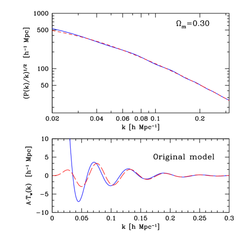
With typical baryon fractions, $f_{b}\sim 0.15$, baryonic oscillations are hardly visible as they make up only $\sim 2\%$ of the multi-component transfer function. This illustrates the main observational challenge in using wiggles as a metric ruler for cosmological investigations. On small scales, $k>0.15h\textrm{Mpc}^{-1}$, Fig. 2 shows that the theoretical wiggle function describes the baryonic oscillations to a satisfactory degree. This is expected, as the transfer function is dominated by the effects of velocity overshoot and Silk damping on these scales and the wiggle function was designed to model these effects. On large scales, $k<0.05\,h\textrm{Mpc}^{-1}$, the BAOs have to cope with competing CDM effects that dominate in these $k$-ranges. As the influence of CDM increases, the transfer function can not be described by baryonic physics alone and further corrections and assumptions have to be applied. Two related effects are:

(1) Turnover-effect: The turnover in the matter power spectrum occurs on the scale $k_{\rm eq}$ of the particle horizon at $z_{\rm eq}$, which coincides with the approximate location of the first wiggle. No observation has hitherto clearly revealed this turnover in spectral power. The main problem in identifying the turnover is mostly due to the fact, that it is located at large scales where precise measurements of spectral power are difficult: the surveys cover too small volumes with slice-like shapes leading to strong smoothing (up to factors of two for the 2dF survey, Percival et al. 2001) and significant leakage in the derived power spectra. Under such conditions it appears quite difficult if not impossible to discriminate the first wiggle from the turnover when even the position of the turnover could not yet been determined to some accuracy. To do this, an excellent signal to noise ratio would be needed as well as precise knowledge of the underlying linear theory matter power spectrum. This includes information of distortions of the power spectrum to the sub-percent level. As a consequence, a model-independent approach like separating the BAOs from the multi-component transfer function with a phenomenological fitting function will only be able to detect the first wiggle when the baryon fraction is about as high as 40 percent or more, as we found with CMBfast simulations. However, we will show that our cosmological test is most sensitive to changes of $w$ on scales around $k=0.1h\textrm{Mpc}^{-1}$. Therefore, the inability of a model-independent approach to detect the first BAO does not matter much as this first wiggle barely contributes any information to the cosmological test, even more as the amplitude of the first wiggle is comparatively low as it is dampened by CDM effects (see Sect. 7).

(2) Phase-shift effects: As mentioned in Sect. 2, the increasing effect of dark matter on large scales introduces a $k$-dependent phase-shift of the BAOs. The theoretical wiggle function (Eq. 1) already includes a phenomenological correction for this effect (replacing $s$ by $\tilde{s}$). A similar effect on the phases, but in the opposite direction, is introduced by the damping of baryons on structure growth. In fact, the main effect of baryons on the multi-component power spectrum is, assuming a standard cosmology, a sharp break in power starting on scales smaller than the turnover. Formally, this break is caused by the rapid decay of the $\tilde{T}_{b}$ component of the transfer function (see Fig. 1). As the break occurs right after the turnover, it is very hard to distinguish shape components from oscillations. For the extraction of BAOs in that scale range we have found that this spectral break must be modeled in detail (with an accuracy on the sub-percent level) or artificial phase-shifts with sizes of the order of interesting $w$ effects are introduced when naive fitting functions ignoring this baryonic backreaction are subtracted from the multi-component power spectrum. Thus the model independent fitting function presented in this work (Eq. 6), but also traditional wiggle-free dark matter transfer functions with a slightly different functional approach like those given in Bardeen et al. (1986) or Efstathiou, Bond & White (1992), introduce artificial phase-shifts of the generic form

$$\left(\frac{\hat{s}}{\tilde{s}}\right)^{3/2}=\;\,0.98\,+\,\left[\frac{5.1\,(\Omega_{\rm m}\,h^{2})^{0.47}}{k\,s}\right]^{3/2}\;,$$ (7)

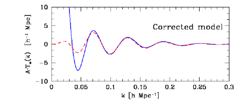
which gives a useful summary of the phase-shifts (about 0.7% at $60h^{-1}{\rm Mpc}$ and 4% at $120h^{-1}{\rm Mpc}$) even for very different baryon fractions. This equation was derived phenomenologically from fits to CMBfast simulations. The second panel in Fig. 2 shows an example for the concordance cosmology. It is seen that the phase-shifts are most prominent at intermediate scales, $k\,<\,0.15\,h\,\textrm{Mpc}^{-1}$, and counteracts the phase-shifts introduced by large-scale CDM potentials. The dashed line in the fourth panel shows the corrected theoretical wiggle function, replacing $\tilde{s}$ in Eq. (1) by $\hat{s}$ from Eq. (7). It is clearly seen that the extracted wiggle function follows the predicted theoretical, and phenomenologically corrected, wiggle function on the 0.5%-level in the range $0.05<k<0.3\,h\,\textrm{Mpc}^{-1}$ which is relevant for a cosmological test of the parameter $w$. In the following, Eqs. (1) and (7) constitute our final theoretical wiggle function which we use in FITEX to match the BAOs extracted from the simulated data.

4 Extracting BAOs under Quasi-Nonlinear Conditions

The simulated data used to test FITEX for BAO extraction under more realistic conditions are provided by the $\rm{\Lambda CDM}$ version of the Hubble Volume Simulations conducted by the Virgo Consortium (Evrard et al. 2002). One billion dark matter particles were simulated with $h=0.7$, $\Omega_{\rm m}=0.3$, $\Omega_{\Lambda}=0.7$, $\Omega_{\rm b}=0.04$, $\Omega_{\rm\nu}=0$, and the normalization of the matter power spectrum, $\sigma_{8}=0.9$, in a cube with a comoving length of $L\,=\,3000$ $h^{-1}\,\rm{Mpc}$ and a mass of $2.25\cdot 10^{12}\,h^{-1}\,\cal{M}_{\odot}$ per particle. The simulations were started with a ‘glass-like’ load (see e.g. Baugh et al. 1995). During the simulation itself, long range gravitational forces were computed on a $1024^{3}$ grid yielding a Nyquist critical frequency of $k_{c}=1.07\;h\,\textrm{Mpc}^{-1}$. The short range gravitational forces were computed via direct summation and softened on a scale of $0.1\;h^{-1}\,\textrm{Mpc}$. We used the $10\times 10\;\textrm{deg}^{2}$ fraction of the XW extended deep wedge which uses periodic boundary conditions from a redshift of $z=4.4$ to provide a survey lightcone up to the redshift $z_{\rm max}=6.8$. The lightcone output comprises of data that includes cluster evolution and thus mimics real life observations. Larger distance from the observer correspond to higher redshifts where structures are less pronounced due to linear and non-linear growth.

Table 1: Parameters of the cubes for the power spectrum estimation. Col. 1: Cube number. Col. 2: Comoving length of the cube (concordance cosmology). Col. 3: Redshift range covered by the cube. Col. 4: Fundamental mode of the discrete Fourier transformation which corresponds to the sample bin size of the power spectrum in $k$ space. Col. 5: Nyquist critical wavenumber of the Fast Fourier Transformation.

Sample	length	$z$-range	$\Delta k$	$k_{c}$
	$[h^{-1}\,\rm{Mpc}]$		$[h\,\rm{Mpc}^{-1}]$	$[h\,\rm{Mpc}^{-1}]$
cube1	200	0.58 – 0.68	0.031	4.0
cube2	226	0.68 – 0.79	0.028	3.6
cube3	256	0.79 – 0.92	0.025	3.1
cube4	291	0.92 – 1.1	0.022	2.8
cube5	329	1.1 – 1.3	0.019	2.4
cube6	373	1.3 – 1.6	0.017	2.2
cube7	423	1.6 – 2.0	0.015	1.9
cube8	479	2.0 – 2.5	0.013	1.7
cube9	500	2.5 – 3.2	0.013	1.6
cube10	500	3.2 – 4.1	0.013	1.6
cube11	500	4.1 – 5.4	0.013	1.6

Figure 3: Upper panel: Power spectra of the matter distribution from the cubes 7 (upper spectrum) to 10 (lower spectrum) of the XW deep wedge N-body simulation with superposed linear theory predictions. The linear matter power spectrum was taken from Eisenstein & Hu (1998). Amplitude corrections for linear structure growth were implemented in the standard manner. For better illustration, the 2nd, 3rd and 4th spectrum is shifted downwards by the factors $\rm{dex}(0.1)$, $\rm{dex}(0.2)$, $\rm{dex}(0.3)$, respectively. The extraction of BAOs described in the main text is restricted to the $k$-range bordered by the two vertical dashed lines. Lower panel: Same as upper panel for the corresponding boosted transfer functions with superposed fits of the phenomenological fitting functions. The fit at $z=2.3$ uses the following parameters: $A=540.0$, $B=35.45$, $k_{1}=-0.32354$, $\alpha=2.493$, $\delta=1.420$.

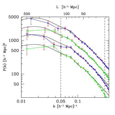
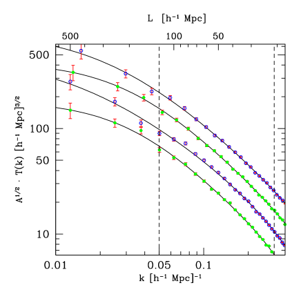
Power spectra, $P_{\rm obs}(k,z,b)$, were estimated at different redshifts and for different galaxy biasing schemes $b$ (see below) with the Fast Fourier Transform using the variance-optimized method of Feldman, Kaiser & Peacock (1994) for cubes along the line-of-sight (LOS) of the XW wedge. All the cubes were selected to fully fit into the lightcone in order to not introduce a non-trivial window function. The parameters of the cubes are given in Tab. 1. Note that the spectroscopic SDSS survey of normal galaxies covers an effective volume which is comparable to cubes with $L\approx 500\,h^{-1}\,{\rm Mpc}$. The errors of the power spectral densities at wavenumber $k$ were estimated with standard mode counting arguments by $\sigma_{P}/P(k)=\sqrt{2\pi}\{1+1/[P(k)\bar{n}]\}/kL$ to provide a first estimate. Here, $\bar{n}$ is the mean comoving particle number density in the box, and $L$ the length of the box. We found that the initial glass load reduces the shotnoise level significantly below the standard Poisson case at redshifts $z>2$ (see Smith et al. 2003). Instead of correcting our spectral estimator for this artifact (see, e.g., Smith et al. 2003), we could in the end neglect its impact on the cosmological test, because our phenomenological fitting function was flexible enough to compensate for the small residuals of this artifact seen in our standard scale range $k<0.3\,h\,{\rm Mpc}^{-1}$.

In order to extract the BAOs from the power spectra $P_{\rm obs}(k,z,b)$, we computed the corresponding boosted transfer functions first, $\sqrt{A(k,z,b)}\,T(k)=\sqrt{P_{\rm obs}(k,z,b)/k}$, assuming a primordial spectrum with $n\,=\,1$ (see below). Fig. 3 shows the estimated power spectra and the corresponding boosted transfer functions for an unbiased dark matter particle distribution in configuration space. Error bars include shot noise and sample variance. In most spectra the 2nd and 3rd BAOs are clearly visible. For $k\geq 0.05\,h\,{\rm Mpc}^{-1}$, the phenomenological fitting function (Eq. 6) can be computed very accurately as it is constrained by a large number of spectral data with relatively small errors, that can be traced reasonably well by a power law. Sample variance is negligible, as in this $k$-range, each spectral point represents the average over a large number of modes. For $k<0.05\,h\,{\rm Mpc}^{-1}$, only a very small number of spectral densities, each estimated with a small number of independent modes, exists and the phenomenological function has to fit a wiggle that coincides with the turnover. Therefore, the results in the range $0<k<0.05\,h\,{\rm Mpc}^{-1}$ vary quite a bit. However, we already excluded this range from the cosmological test (see vertical dashed lines in Fig. 3 and the discussion at the end of Sect. 3).

The extracted BAOs for the four cubes 7-10 of the XW deep wedge simulation corresponding to the redshifts $z=1.8$-3.7 are shown in Fig. 4. Spectral densities in the range $0.05<k<0.3\,h\,{\rm Mpc}^{-1}$ which is relevant for unbiased cosmological tests are plotted (dots) together with the theoretical wiggle function (Eqs. 1,7) multiplied by an appropriate amplitude $\sqrt{A}$ (solid line). We see that even for very large galaxy samples filling a box-like survey volume with a length of $L=500\,h^{-1}\,{\rm Mpc}$ error bars are mainly determined by sample variance and are of the same order as the amplitudes of the BAOs. Therefore, only surveys with significantly larger survey volumes can show the BAOs with higher significance.

Figure 4: Extracted baryonic oscillations of dark matter particles (dots) with error bars including shot noise and sample variance at different redshifts ranging from $z\,=\,1.8$ (upper left panel) to $z\,=\,3.8$ (lower right panel). Superimposed is the theoretical wiggle function (Eq. 1) with an appropriate amplitude.

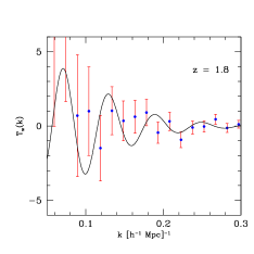
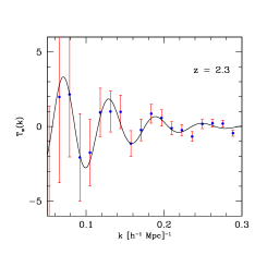
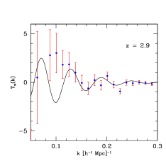
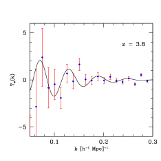
We further see that the amplitudes of the wiggle functions in Fig. 4 decrease with increasing redshift, due to growth suppression (we verified the amplitude change with $z$ according to standard linear structure growth). This is a direct consequence of the fact, that distortions of the power spectrum are directly translated into the boosted transfer function and thus into distortions of the amplitude of the BAOs. To see how this works and how deviations from the assumed primordial spectrum with $n=1$ affect the wiggle function, we rewrite the primordial spectrum in the form $k^{1+2\epsilon}$ with $|\epsilon|$ small compared to unity. For the assumed power spectrum, $P(k,z,b)=A(k,z,b)k^{n}T^{2}(k)$, this choice gives

$$\sqrt{\frac{P(k,z,b)}{k}}-F(k,b,z)=\sqrt{A(k,z,b)}k^{\epsilon}\frac{\Omega_{\rm b}}{\Omega_{\rm m}}T_{\rm w}(k)\,,$$ (8)

where the phenomenological function (Eq. 6) effectively fits the amplitude and shape-dependencies (see Eqs. 2, 3)

$$F(k,z,b)=\sqrt{A(k,b,z)}k^{\epsilon}\left[\frac{\Omega_{\rm c}}{\Omega_{\rm m}}T_{\rm c}(k)+\frac{\Omega_{\rm b}}{\Omega_{\rm m}}\tilde{T}_{\rm b}(k)\right]\,.$$ (9)

It is seen that the phases of the wiggle functions remain unchanged by the FITEX procedure. This result is shown in Fig. 5 where the extracted oscillations from power spectra with different spectral index models in the primordial power spectra are plotted. The oscillations were retrieved by calculating a power spectrum with a spectral index $n=1$ (solid line), an index of $n=0.9$ (long dashed line) and a simple running spectral index model $k^{1-0.1\ln{k}}$ (short dashed line) and applying the FITDEX method. The parameters are chosen to conservatively cover the range of primordial power spectra not excluded by WMAP 3rd year data (see Bridges et al. 2006).

Figure 5: Wiggle extraction from power spectra with different primordial $k$ dependencies. The resulting oscillations using FITDEX on primordial models with a spectral index $n=1$ (solid line) is compared to a model with different spectral index $n=0.9$ (long dashed line) and a running spectral index with $\alpha=0.1$ (short dashed line).

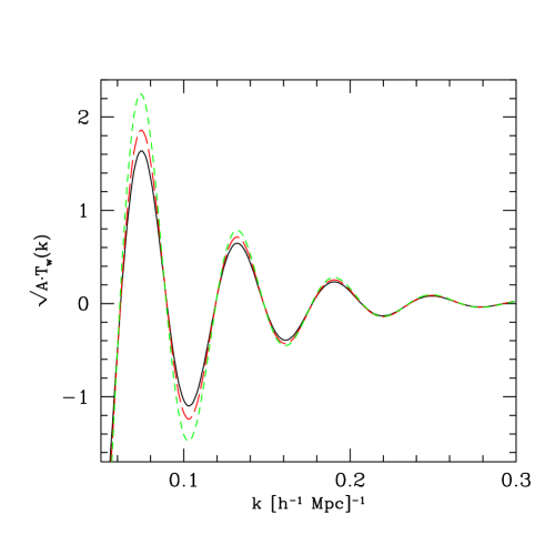
Only the amplitudes of the wiggle functions are modulated by possibly scale-dependent factors. Although a lot of interesting information about galaxy formation and cosmology is contained in the amplitude factors of the wiggle function, we skip this detail here and perform an amplitude rescaling, $\sqrt{A(k,z,b)}k^{\epsilon}\Omega_{\rm b}/\Omega_{\rm m}\rightarrow\sqrt{A(k,b,z)}$, with $A(k,z,b)$ being a basically arbitrary function after rescaling, summarizing distortions like structure growth, galaxy biasing, redshift space effects, deviations from the Harrison-Zel’dovich case etc. Thus, with FITEX we are not deriving a pure undistorted wiggle function, but a spectrum which is subject to all the distortions that work on the power spectrum.

While the oscillations extracted from the Hubble Volume Simulations are consistent with the theoretical template, the error bars prevent a precise evaluation of the accuracy of FITEX (all 4 cubes will be combined later, see Fig. 15). To get a better estimate of non-linearities that might wash out wiggles at higher $k$ values, we use a non-linear analytic form of the power spectrum. This was computed by Jeong & Komatsu (2006) using 3rd-order perturbation theory, which is able to model non-linear N-body matter power spectra to better than 1% at $z>2$ and $k<0.3\,h\,{\rm Mpc}^{-1}$.

Figure 6: BAO extracted from an analytic power spectrum of Jeong & Komatsu (2006) that includes non-linear growth at $z=2.3$ (dots). The continuous line is the theoretical wiggle function derived in Sect. 2, multiplied by an appropriate amplitude. See the main text for a more detailed discussion of the treatment of the amplitudes of the wiggle function and the analytic power spectrum.

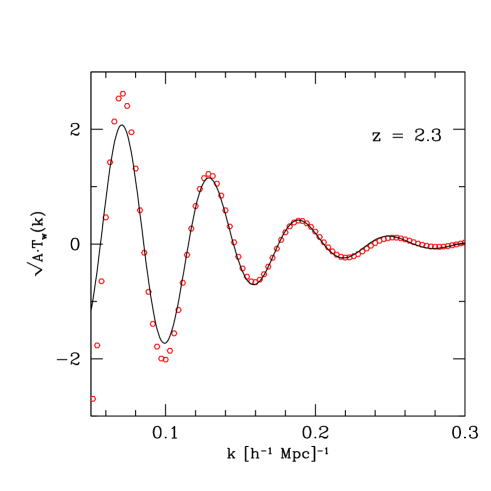
Figure  6 shows the results of the FITEX extraction applied to the analytic non-linear power spectrum using Hubble Volume parameters. As expected, the amplitude deviates from the theoretical prediction at small $k$-values, where the shape contribution of the baryons dominates (see. Fig. 1), but the phase of the oscillations in the analytical non-linear function is recovered to better than 1% accuracy. This clearly shows, that, at least in theory, FITEX is able to model non-linear effects and recover the oscillations with high accuracy.

As an additional test, the power spectrum of the Hubble Volume Simulation (OCTANT data), a wedge covering on eighth of the sky from $z=0-1.3$ including redshift-space effects, was computed with about 60 million particles in a fast Fourier box with a legnth of $1600\,h^{-1}\,\rm{Mpc}$ and the FITDEX algorithm used to extract the oscillations (Fig. 7). The oscillations can be seen, although non-linear growth is heavily washing out the wiggles at $k>0.22\,h\,{\rm Mpc}^{-1}$.

Figure 7: Extracted BAOs using the Hubble Volume Simulation covering one eighth of the sky from redshift 0 to 1.3. Error bars include sample variance and shotnoise but do not cover washing out effects introduced by the correlation of modes through non-linear growth and distant observer approximation.

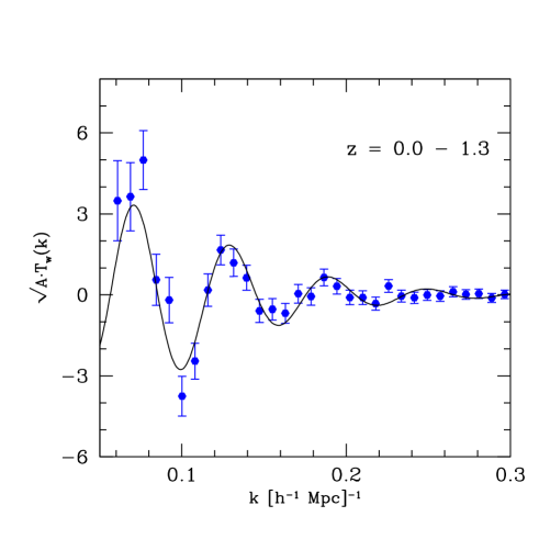
Furthermore, we see a very good correspondence between a FITEX-extracted wiggle function obtained from N-body simulations as well as the analytic non-linear power spectrum and the theoretical wiggle function of FITEX (Eq. 1) in the HETDEX redshift range. Both linear and non-linear structure growth change the power spectrum and thus the BAOs, but FITEX still gives quite stable and easy to analyze results for the 2nd to 5th BAO. The presence of the BAOs is consistent with the results of recent simulations of e.g. Springel et al. (2005) and Seo & Eisenstein (2005). However, no specific method to extract the BAOs was applied and their simulations did not include lightcone effects. In the following we concentrate on the effects of redshift space and scale-dependent galaxy biasing on the results obtained with FITEX.

5 Extracting BAOs in Redshift Space

The main problem in relating redshift space coordinates with comoving coordinates is the differentiation between red-shifting due to the expansion of the Universe and red-shifting due to peculiar velocities of the measured particles. Two effects might be important.

(1) In the linear regime and in combination with the distant observer approximation, peculiar velocities introduce a boosting factor $\beta$ along the LOS. Only the $k$-modes parallel to the LOS, $k_{\parallel}$, are boosted by the square of the factor $1\,+\,\beta(z,b)k_{\parallel}^{2}/(k_{\parallel}^{2}\,+\,k_{\perp}^{2})$ with $\beta(z,b)=-d\ln D(z)/[d\ln(1\,+\,z)b(k,z)]$, $D(z)$ the linear structure growth, and $b(k,z)$ the biasing parameter (Kaiser 1987).

(2) In the non-linear regime, velocity dispersion of galaxies in (partially) virialized structures cause the well-known ‘fingers of God’ effect in redshift space. We assume that the effect is mainly restricted to small scales and is describable by a simple exponential damping of the power spectrum by the factor $\exp(-\alpha k^{2}_{\parallel})$. Here, the redshift-dependent parameter $\alpha$ gives a measure of the average pairwise velocity dispersion in the given redshift shell.

Figure 8: Redshift space spectra divided by their corresponding real space spectra at different redshifts (filled areas). Overplotted lines represent the best fit of the kernel of Eq. (10).

The combination of (1) and (2) constitute one version of the standard dispersion model of peculiar velocities which relates the one-dimensional redshift and real space power spectra by

$$P_{\rm s}(k,z,b)\,=\,P(k,z,b)\,\int_{0}^{1}d\mu\left[1\,+\,\beta(z,b)\mu^{2}\right]^{2}\,e^{-\alpha(k\mu)^{2}}\;,$$ (10)

where $\mu$ is the cosine between the direction of the actual wavevector and the LOS, i.e., $\mu k=k_{\parallel}$, and $k^{2}=k_{\parallel}^{2}+k_{\perp}^{2}$ (for more detailed models see Scoccimarro 2004). On large scales, the real space power and thus the wiggle function is boosted in a $k$-independent manner (Kaiser factor). On small scales, the power spectrum is dampened in a $k$-dependent manner by the factor $0.5\sqrt{\pi}\,{\rm erf}(\alpha k)/\alpha k$, with erf the standard error function of statistics. In Schuecker, Ott & Seitter (1996) it is shown that Gaussian redshift errors can be described with the same model (for $\beta=0$). Eq. (10) suggests that only the amplitudes but not the phases of the BAOs can be changed by this type of redshift space distortion.

Figure 9: Ratios of boosted redshift and real-space transfer functions for different redshifts. As expected, the redshift space effects increase with decreasing redshift in a smooth manner. Increasing ratios at high redshifts are an artifact caused by the glass-like initial load of the N-body simulations. To illustrate the relation between redshift space effects and amplitudes of BAOs, the ratio between BAOs and the transfer function is plotted in the upper panel.

Figure 10: Comparison of wiggle functions at $z=1.2$ (upper panel) and $z=2.3$ (lower panel) obtained from real space (filled circles and continuous lines) and redshift space (open circles and dashed lines). Note the overall boost of the wiggle functions by redshift space effects which, however, leaves the phases of the BAOs invariant. The non-linear growth effects, start to wash out the wiggles at $k>0.2\,h\,\rm{Mpc^{-1}}$ in the upper panel.

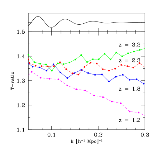
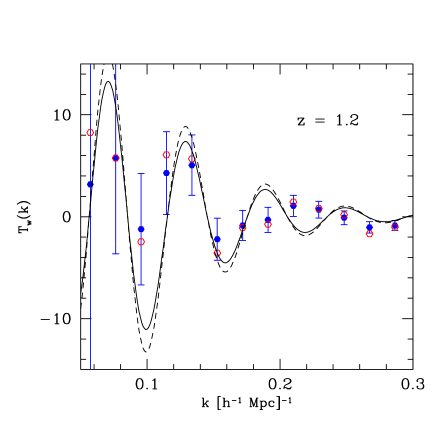
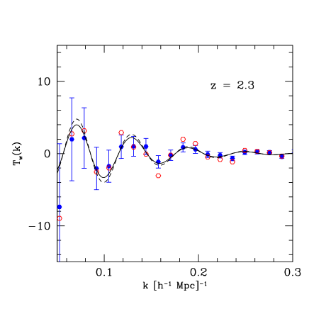
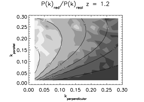
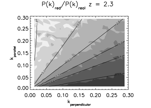
Figure 8 illustrates the combined effect in more detail. Two redshift space power spectra, as obtained from the Hubble Volume Simulation, were divided by their corresponding real space spectra at different redshifts and plotted as filled areas. The kernel of Eq. (10) was fitted to this ratio and the best fit results superposed (black solid lines). We found that the model is accurate on the 5%-level over the complete redshift range. For $z>2$, the parameter $\alpha$ is virtually zero because no virialization had time to take place on the scales shown. As redshift decreases, galaxy clusters start to form and virialize and the $\alpha$ parameter starts to distort not the amplitude in the two dimensional power spectrum depending on the angular component, like $\beta$ does, but changes the amplitude depending on the modulus of the $k$ vector. This means that the shape of the wiggles could be influenced by this effect as the amplitude of the power spectrum and thus the amplitude of the wiggles is dampened at high $k$-values.

Fortunately, this anisotropy only gradually changes the amplitude of each consecutive mode over which is averaged in a $k$-shell from perpendicular to parallel modes. This is illustrated in Fig. 9 where the ratios of boosted transfer functions are plotted. A rough idea about the relation between redshift space effects and the amplitudes of BAOs is provided by the ratio between BAO and the transfer function plotted in the upper part of Fig. 9.

Two examples of wiggle functions boosted by redshift-space effects and extracted with FITEX are plotted in Fig. 10. The result of the anisotropic redshift space is that modes with a more parallel component get more weight than those with a more perpendicular component, which are not boosted. Whereas the overall shape of the wiggle function appears to be slightly changed, the phases of the wiggles are not distorted at all. Instead, the whole wiggle function receives a boost of the monopole component of the Kaiser factor.

The fitting function is obviously able to model the redshift space distortions on the sub-percent level and oscillations can be derived. If the wiggles were not extracted with FITEX-like methods but by dividing the observed power spectrum by a standard non-oscillatory linear theory power spectrum, as was done by in Springel et al. (2005, Fig. 10) and Cole et al. (2005, Fig. 13), the baseline of the oscillations would start to depart from zero at smaller scales. Such an oscillation spectrum could not easily be used in a cosmological test as it fit only nontrivial theoretical model spectra.

6 Extracting BAOs from Biased Samples

In the Hubble Volume, CDM particles are simulated. What is actually observed are galaxies made out of dark matter and baryonic matter, especially in the case of the proposed HETDEX survey, where Lyman-$\alpha$ emitting galaxies are used as tracers of the underlying matter distribution. Because of the different properties of dark matter and baryonic matter (Benson et al. 2000, Le Delliou et al. 2006), both need not necessarily follow exactly the same density distribution.

To test the stability of FITEX under such conditions, we introduce some sort of biasing into the N-body simulations. Formally, biasing is described by the mean biasing function (Dekel & Lahav 1999),

$$b(\delta_{d})\,\delta_{d}\;=\;\langle\delta_{g}\,|\,\delta_{d}\rangle\;=\;\int d\delta_{g}\,P(\delta_{g}\,|\,\delta_{d})\,\delta_{g}\;,$$ (11)

that relates the dark matter distribution $\delta_{d}$ to the galaxy distribution $\delta_{g}$ (Somerville et al. 2001). Here, $P(\delta_{g}|\,\delta_{d})$ is the local conditional biasing distribution, i.e. the probability that a certain matter density contrast $\delta_{d}$ with a variance $\sigma_{d}^{2}$ is converted into a galaxy contrast $\delta_{g}$ with a variance $\sigma_{g}^{2}$. The biasing function can also be expanded into the moments, $\hat{b}=\langle b(\delta_{d})\,\delta_{d}^{2}\rangle/\sigma_{d}^{2}$, and $\tilde{b}^{2}=\langle b^{2}(\delta_{d})\delta_{d}^{2}\rangle/\sigma_{d}^{2}$, with the biasing scatter $\sigma_{b}^{2}=\langle(\delta_{d}-\langle\delta_{g}|\delta_{d}\rangle)^{2}\rangle/\sigma^{2}_{d}$. Any local, non-linear and stochastic biasing relation can be described by these moments to second order. While $\tilde{b}/\hat{b}$ is a measure for the non-linearity and $\sigma_{b}/\hat{b}$ a measure of the scatter, the parameter $\hat{b}$ characterizes the linear biasing such, that if $\hat{b}=\tilde{b}$, then $\delta_{g}(\@vec{x})=\hat{b}\delta_{d}(\@vec{x})$ (Wild et al. 2005).

Figure 11: Ratios of biased and unbiased boosted transfer functions for two samples with different scale-dependent biasing at $z=2.3$. A factor of 2 was subtracted from the strong bias (dashed line) for enhanced visibility, while the weak biasing (solid line) remains unchanged. The theoretical wiggle function is plotted on top of the figure to illustrate the scale of the biasing effects.

Figure 12: Boosted wiggle functions extracted with FITEX and theoretical wiggle functions for the unbiased sample (filled circles and continuous line), for the strongly biased sample (triangles and shot-dashed line) and for the less biased sample (open circles and long-dashed line). The theoretical wiggle functions are multiplied by the $\hat{b}$-moment of the biasing function.

We use the simple stochastic and slightly non-linear Eulerian biasing scheme (e.g. Cole et al. 1998, Yoshida et al. 2001). First, local overdensities for each dark matter particle are computed by smoothing the distribution with a Gaussian, $\textrm{exp}(-r^{2}/2r_{0}^{2})$ and $r_{0}=3\,h^{-1}\,\textrm{Mpc}$. The overdensities $\delta_{d}$ are then transformed into normalized overdensities, $\nu=\delta_{d}/\sigma_{d}$, with $\sigma_{d}$ being the root mean square of the $\delta_{d}$-values. Finally, a function is introduced that describes the probability of a dark matter particle with overdensity $\delta_{d}$ to be tagged as a ‘galaxy’, $P(\nu)\sim(\nu-\nu_{c})^{\alpha}$, with $\nu_{c}$ being a threshold at which the probability is set to zero. This simulates the lower probability of galaxies forming in low density regions like voids. The parameter $\alpha$ controls the stochastic spread of the biasing function as well as its non-linearity. A value of $\alpha\,=\,0.2$ is a good compromise between reasonable non-linearity and a comparably tight spread. Two samples with $\nu_{c}\,=\,-0.2$ and 0.6 were generated. Both parameters, $\alpha$ and $\nu_{c}$, were adjusted to model the biasing parameters and number densities found by observation. SUBARU data (Hamana et al. 2004) suggests a comoving LAE density of $\bar{n}\,=\,0.00301\,\pm\,0.00194\,h^{3}\,\textrm{Mpc}^{-3}$ and a biasing parameter of $\hat{b}\,=$ 4-5 at a redshift $z\,=\,5$, which should decrease slightly with redshift. As discussed in Sect. 4 the biasing function $b(\delta_{d})$ should translate into a boost of the power spectrum $b^{2}(k,z)$. Because the average slope of the biasing function is $\hat{b}$, to first order we expect $P_{\rm bias}(k)=P(k)b^{2}(k,z)\sim P(k)\hat{b}^{2}(z)$.

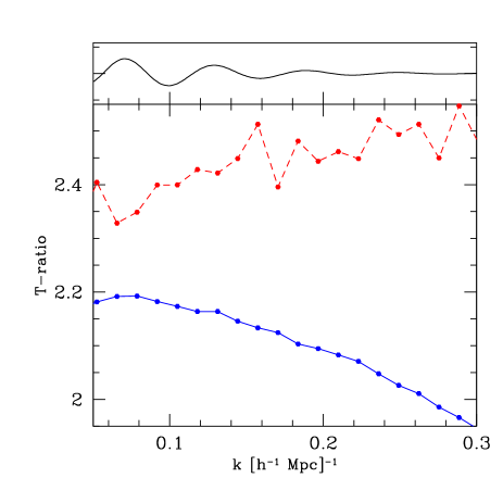
The two prescriptions lead to a biasing that either decreases or increases with $k$ (see Fig. 11). Both values are consistent with the calculated $\hat{b}$ parameter. The comparatively strong scale dependence of the biasing becomes evident when the ratios of the boosted transfer functions are compared with the ratio of the wiggle amplitude to the transfer function plotted on top of Fig. 11.

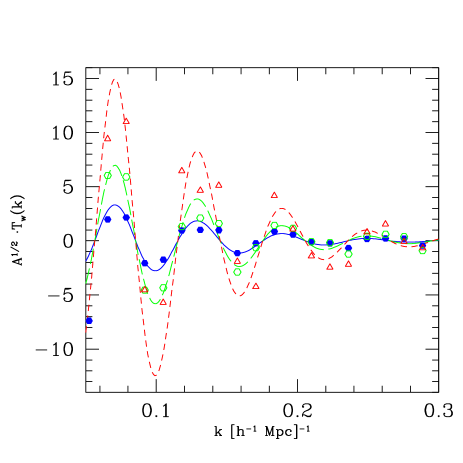
Figure 12 illustrates, that FITEX extracts BAOs even from biased galaxy distributions. Plotted are the wiggle functions of the less strongly biased sample (open circles), the more strongly biased sample (open triangles) and the unbiased sample (filled circles) at $z\,=\,2.3$. The unbiased and biased oscillations vary because of shot noise, as the biased samples have a 2 and 10 times lower point density, respectively. Superimposed are the theoretical wiggle functions (Eq. 1), normalized to the unbiased wiggle function (continuous line) and multiplied by the first moment of the biasing, $\hat{b}$ (dashed lines). The boost of the power spectrum obviously translates into an amplitude boost of the BAOs. As in redshift space, only the phenomenological fitting function as used in FITEX extracts the BAOs with a zero baseline, unlike when using a linear theory power spectrum.

However, not only the overall boost of the power spectrum, but also the $k$-dependency of the biasing function should directly affect the amplitude of the BAOs. We tried to verify this by fitting the $T_{w}(k)$ function supplemented by a ‘linear biasing model’ to describe the extracted wiggle function $T_{\rm ex}(k)=(a_{0}\,+\,a_{1}\,k)T_{w}(k)$. We notice that both parameters $a_{0}$ and $a_{1}$ are highly degenerate, mainly due to the fact that only data points at the extrema of the wiggle function significantly contribute to the fit. Data points at or near the nodes of the wiggle function are very insensitive to changes of the amplitude. Due to the degeneracy, any amplitude $a_{0}$ can easily be compensated by an appropriate value of the parameter $a_{1}$. Though the full fits had the expected slopes, the effects were very small and of no significance for the cosmological test. We may thus conclude that in a cosmological test, which is mostly about detecting phase-shifts, it seems to be enough to fit the theoretical wiggle function with only an amplitude parameter, when the $k$-dependent biasing is as weak as simulated here. However, more realistic simulations are needed to analyze higher order effects.

7 Cosmological Tests with BAOs

The cosmological test compares the phases of the extracted BAOs with the theoretical wiggle function, projected onto the hypersphere of the observer. As the theoretical template does not model the amplitude of the oscillations with high accuracy, we are not able to include amplitude effects in the cosmological test and marginalize over the wiggle amplitude. Future tests should include this parameter, which is sensitive to $w$ by e.g. structure growth.

A general feature of the test is that one first has to assume a certain reference cosmology to get the metric scale of the wiggle function from the data, and to perform in a second step the comparison of the metric scale of the theoretical wiggle function relative to the chosen reference cosmology (Glazebrook & Blake 2005). In the present paper, we are interested in the performance of the BAOs extracted with FITEX in constraining the redshift-independent part of the $w$ parameter of the dark energy. The amplitude of the theoretical function is also fitted but later marginalized. The remaining cosmological parameters are fixed to their values given at the end of Sect. 1.

As metric scales, comoving distances of the BAOs parallel and perpendicular to the LOS are used. Recall that in the plane-parallel or distant observer approximation, comoving distances between two points with the same angular positions but different redshifts are $x_{\parallel}=\int_{z_{1}}^{z_{2}}\frac{dx}{dz}dz=\frac{c}{H_{0}}\int_{z_{1}}^{z_{2}}\frac{dz}{E(z)}$, where $H(z)=H_{0}E(z)$ is the Hubble parameter at redshift $z$ and $E(z)$ the $w$-dependent transformation of the Hubble constant, $H_{0}$, from redshift zero to $z$ (e.g., Peebles 1993). To compute not distances between two points in space with different redshifts, but parallel scaling factors between the two sets of cosmologies denoted by primed and unprimed symbols, one has to take the limit $\Delta z=z_{2}-z_{1}\rightarrow 0$, which yields

$$x^{\prime}_{\parallel}\,=\,x_{\parallel}\,\frac{dx^{\prime}}{dx}\,.$$ (12)

Comoving perpendicular separations represent distances two points with the same redshift but different angular positions are separated, $x_{\perp}=\theta\int_{0}^{z_{2}}\frac{dx}{dz}\,dz$, where $\theta$ is the angle between the two points. The scaling relation for the perpendicular component between two cosmologies thus becomes

$$x^{\prime}_{\perp}\,=\,x_{\perp}\,\frac{x^{\prime}}{x}\,.$$ (13)

In Fig. 13 the transformation ratio of the wiggle function is plotted at different redshifts for two cosmologies that differ from the reference model only in $w_{0}$ (the redshift-independent part of $w$). The reference model is the concordance cosmology. Fig. 13 shows that the largest deviations from the reference model appear at redshifts in the range $0.5<z<1.5$. Differences in parallel and perpendicular scaling introduce anisotropies that could be measured, too (see below).

Figure 13: Transformation of perpendicular (solid) and parallel (dashed) distances in comparison to the concordance model with $w_{0}\,=\,-0.7$ (upper part) and $w_{0}\,=\,-1.3$ (lower part).

Figure 14: Scaled wiggle functions at $z\,=\,2.5$ for $w_{0}=-0.7$ (dashed line) compared to the $w_{0}\,=\,-1$ cosmology (solid line, top panel). The normalized modulus of the difference between the reference cosmology and the scaled cosmology is shown in the bottom panel. The dashed vertical lines mark the region relevant for the cosmological test.

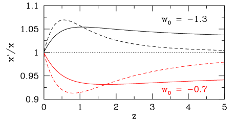
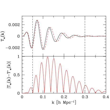
Figure 14 shows the scaled wiggle function at redshift $z=2.5$ for $w_{0}=-0.7$. The reference and the distorted wiggle function are plotted. Note that an elongation of the coordinates in real space leads to a compression of the coordinates in $k$-space and vice versa. In the upper panel, it can be seen that the wiggle function gets more and more out of phase as $k$ increases. Thus the sensitivity of a cosmological test should increase at high values of $k$. However, the amplitudes of the oscillations decrease exponentially with $k$ (e.g., Silk damping). This can be seen in the lower panel of Fig. 14 where the scaled wiggle function is subtracted from the reference ($w_{0}=-1$) wiggle function: Though the difference in phase is increasing, the amplitude decreases so fast that the difference between the projected oscillations increases at small values of $k$ and decreases at high values of $k$.

The present version of the cosmological test comprises the following steps: (1) Angular and redshift coordinates of the ‘observed’ (simulated) data are transformed into comoving coordinates using a concordance model as the reference cosmology. (2) The comoving data sample is Fourier-transformed to estimate the boosted transfer functions. (3) BAOs are extracted with FITEX. (4) The theoretical wiggle function is computed for the corresponding cosmological model. (5) The parallel and perpendicular scaling factors between the test cosmology and the reference cosmology are computed at the redshift of the data sample. (6) The theoretical wiggle function is scaled by constructing a three-dimensional wiggle function, scaling each mode and collapsing it to one dimension. (7) The observed wiggle function is compared to the re-scaled theoretical wiggle function assuming Gaussian statistical errors ($\chi^{2}$ test). Only the steps (4-7) have to be repeated to test a different cosmology, allowing a fast test of various parameters.

Note that the three-dimensional wiggle function is only constructed to simulate the effects of different parallel and perpendicular scaling factors. It does not address the anisotropy introduced by redshift space effects, because we found that this only boosts the various modes but not change the phases of the theoretical wiggle function (see Sect 5). The boost effect of the redshift space distortions, along with other boosting effects like biasing and growth suppression, will force us to add an additional parameter to the cosmological test.

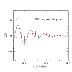
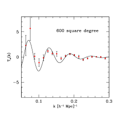
Figure 15 shows in the upper left panel the combined wiggle function of the four XW wedge cubes of the Hubble Volume Simulation. The combination is performed by averaging over $k$-bins of discrete size. The errors represent the standard deviation of all wiggle points in the corresponding $k$-bins. After averaging, the 2nd to 5th BAOs are now clearly visible. We thus conclude that a volume at least 4 times larger than SDSS has to be sampled in order to see the BAOs with FITEX with high significance. One has to keep in mind, though, that our cubes are located at much higher redshifts, where the smoothing effect of non-linear structure growth is obviously much smaller. We also neglected the fact, that larger sky coverages reduce the sizes of the fundamental modes, leading to higher (better) sampling rates of BAOs.

Figure 15: Combined wiggle functions from the four Hubble Volume cubes. The upper left panel shows the combined data point (dots) with self-consistent error bars for the 100 square degree field. The upper right panel shows expected error bars for 200 square degrees and the lower row with error bars for 300 and 600 square degrees, respectively. The continuous lines are the theoretical wiggle functions for the reference (concordance) cosmology.

With the 100 square degree sample, the possibility of data points appearing at positions which severely inhibit the accuracy of the cosmological test is relatively high, due to the high sample variance. Especially as only a few data points, which are far away from positions where theoretical wiggle functions of different cosmological models intersect, have great statistical weight in the cosmological test. This fact is shown in Fig. 14, where the modulus of the difference between the theoretical transfer functions for two models depending on position in $k$-space is plotted.

Figure 16: $\chi^{2}$ distributions for the $w_{0}$ parameter obtained after marginalization over the amplitude parameter and for different conditions of BAO extraction. Short-dashed line: dark matter distribution in configuration space over 100 sq. deg obtained from the simulation of dark matter particles in configuration space. Continuous line: biased particle distribution in redshift space over 100 sq. deg. Dotted line: biased particle distribution in redshift space over 300 sq. deg (extrapolation). Dashed-dotted line: biased particle distribution in redshift space over 600 sq. deg (extrapolation). The horizontal dashed line marks the $1\sigma$ error level.

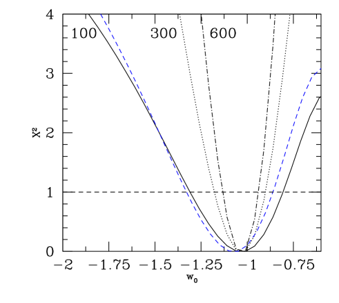
Figure 16 shows the results of the cosmological test obtained with BAOs extracted with FITEX under different survey conditions. For surveys covering 100 square degrees we would expect errors of $\sigma_{w_{0}}=0.25$. The asymmetry of the error distributions directly reflects the increased sensitivity of metric scales on $w$ for $w_{0}>-1$ compared to $w_{0}<-1$. At these $w_{0}$ values, the theoretical wiggle function gets quite compressed, so that at large $k$ values the amplitude decreases rapidly due to Silk damping. When $w_{0}\rightarrow-\infty$, the theoretical wiggle function formally mimics the case of zero amplitude, so that low values of $w_{0}$ are excluded with about the same significance as the “no-wiggle” case of zero amplitude. The minima of all error distributions plotted in Fig. 16 are slightly off-set from the input $w_{0}=-1$ value, but well within all formal $1\sigma$ ranges.

Note that the constraints given above are based solely on the phases of the oscillations in the one-dimensional power spectrum, assuming perfect knowledge of the sound horizon at drag epoch. The $w$-constraints are expected to further improve when the full two dimensional redshift space effects as well as the amplitudes of the BAOs are used.

Perhaps the most important result of the present investigation is the comparatively small decrease of only 8% of $\sigma_{w_{0}}$ when comparing the $w$ test with unbiased matter distributions in configuration space, (dashed line in Fig. 16) i.e., the simplest survey condition, with the test that includes all aforementioned effects (solid line). The robustness of the FITEX method to extract BAOs from boosted transfer functions with phenomenological fitting functions is mainly related to the fact that only the amplitudes of the wiggle functions are boosted by redshift-space and biasing effects, but the phases are not affected.

To give an idea of the performance of FITEX based on surveys of larger size, we extrapolated the results from the 100 square degree data. The upper right panel of Fig. 15 shows wiggle functions extracted from the 100 square degree data but with error bars expected for 200 - 600 square degrees. The error bars were extrapolated by scaling them according to the expected number of additional $k$-modes. The different survey fields are thus assumed to be not adjacent.

Figure 15 shows that increasing the survey volume to 200 square degrees does not reduce the error bars significantly, still allowing for crucial data points at peaks of the oscillating wiggle function to be reduced to zero amplitude. Error bars are still of the same order of magnitude as the oscillations. Only at 300 square degrees (lower left panel), the probability for smoothing out the oscillations due to statistical errors gets considerably low. Following our extrapolations, for a survey of 600 square degrees, the errors are expected to get much smaller than the amplitude of the oscillations and the chance of statistical deviations from the predicted function is of an order of magnitude that allows for very accurate cosmological probing.

The accuracies of the $w_{0}$ parameter (Fig. 16) range from $\sigma_{w_{0}}=0.25$ for 100 sq. deg which corresponds to 3 SDSS volumes, to $\sigma_{w_{0}}=0.09$ for 600 sq. deg, corresponding to 21 SDSS volumes. These results are obtained for biased samples in redshift space, i.e., the most complex survey condition. The improvement is directly related to the larger number of independent $k$-modes in larger survey volumes and is consistent with results obtained with Monte-Carlo simulations (Blake & Glazebrook 2003, their Fig. 8).

Future studies should also investigate the various parameters of the cosmological test to get constraints under less strong priors.

8 Discussion and Conclusions

We have seen that it is critical for the extraction of BAOs to either fit a phenomenological function to the continuum of the boosted transfer function (FITEX), or to calculate the shape of the boosted transfer function, including all distortions down to the sub-percent level. The latter approach has been carried out recently. Glazebrook & Blake (2005), Hütsi (2005), and Springel et al. (2005) used a linear theory power spectrum and divided the ‘observed’ data by this reference. Almost the same approach, but with the addition of linearizing the observational data before the division, to correct for non-linear structure growth was used in Angulo et al. (2005). There are two drawbacks of this method:

First, the ratio of a complex power spectrum and a reference power spectrum does not resemble a wiggle function as defined in the text, but something more complicated (see Eq. 4). The simple form of the theoretical wiggle function (Eq. 1) is strongly deformed by both the chosen transfer function of the reference spectrum and the distortions introduced by redshift space and galaxy biasing. These distortions make the comparison with theoretically expected model spectra unnecessarily complicated. FITEX transforms the observed power spectrum into a boosted transfer function where the subtraction of a non-oscillating phenomenological continuum function is directly related to $T_{w}(k)$, multiplied by an amplitude factor.

The second drawback is the linear theory power spectrum itself. By computing a correct shape of the power spectrum, one has to rely strongly on assumptions about the nature of the dark matter and various other physical processes. The method is no more the ‘assumption free’ approach that was intended. Furthermore, the calculation of the amplitude factor that includes all the distortions ranging from linear structure growth, non-linear structure growth to redshift space distortions and biasing is a problem. This calculation has to be accurate to the sub-percent level, as the oscillations themselves make up only $\sim\,2\%$ of the transfer function.

A more phenomenological approach was conducted by White (2005). He assumed that redshift space distortions as well as linear and non-linear structure growth could be calculated with reasonable accuracy. Leaving only the ratio between dark matter power spectra and ‘galaxy’ power spectra, he found that one can fit this ratio with about 2% accuracy using a cubic polynomial. This adds further evidence that a phenomenological approach can model power spectrum distortions without assuming much about the physics of the distortions themselves.

With the FITEX method, we have shown that one is able to extract the BAOs without any strong priors on the nature of dark matter or the shape of the power spectrum from the complex multi-component transfer function. All the aforementioned effects are modeled by the continuum function and need not be known very accurately, as long as the phases of the oscillations are not distorted or washed out. This extraction is accurate on the sub-percent level within $k$-ranges relevant for the cosmological test. Furthermore, FITDEX is able to disentangle phase information from amplitude information which could in the future be used to test the geometry of the Universe on the one hand and the growth history on the other hand. This type of cosmological test could be used to discriminate Dark Energy from Modified Gravity theories.