Past and present star formation in the SMC: NGC 346 and its neighborhood

Abstract

In the quest of understanding how star formation occurs and propagates in the low metallicity environment of the Small Magellanic Cloud (SMC), we acquired deep F555W ($\sim$V), and F814W ($\sim$I) HST/ACS images of the young and massive star forming region NGC 346. These images and their photometric analysis provide us with a snapshot of the star formation history of the region. We find evidence for star formation extending from $\approx$10 Gyr in the past until $\approx 150\,{\rm Myr}$ in the field of the SMC. The youngest stellar population ($\sim 3\pm 1\,{\rm Myr}$) is associated with the NGC 346 cluster. It includes a rich component of low mass pre-main sequence stars mainly concentrated in a number of sub–clusters, spatially co–located with CO clumps previously detected by Rubio et al. (2000). Within our analysis uncertainties, these sub–clusters appear coeval with each other. The most massive stars appear concentrated in the central sub–clusters, indicating possible mass segregation. A number of embedded clusters are also observed. This finding, combined with the overall wealth of dust and gas, could imply that star formation is still active. An intermediate age star cluster, BS90, formed $\sim 4.3\pm 0.1\,{\rm Gyr}$ ago, is also present in the region. Thus, this region of the SMC has supported star formation with varying levels of intensity over much of the cosmic time.

1 Introduction

The Small Magellanic Cloud (SMC) is an excellent laboratory to investigate the star formation (SF) processes and the associated chemical evolution in dwarf galaxies. Its current sub-solar chemical abundance (Z=0.004) makes it the best local counterpart to the large majority of dwarf irregular (dIrr) and Blue Compact Dwarf (BCD) galaxies, whose characteristics may be similar to those in the primordial universe. Because the SMC is part of a triple system, its star formation can be triggered by interactions with the Milky Way (MW) and the Large Magellanic Cloud (LMC). This kind of interactions might have been very frequent in the past, if galaxies are building up via hierarchical mergers.

The SMC proximity allows us to resolve into single stars the youngest and most compact star clusters, down to the sub solar mass regime. Young star clusters have been extensively studied in the MW and in the LMC, and a direct comparison of the characteristics of these clusters with those of the SMC allows us to address fundamental issues such as the universality of the initial mass function (IMF), and the occurrence of primordial mass segregation within star forming regions.

In this paper we present an in–depth study of the stellar content of NGC 346 ($\alpha_{2000}=$ 00:59:05.2; $\delta_{2000}=-$72:10:28). This star cluster is an outstanding benchmark for star formation studies. It is an extremely young, ($\sim$3 Myr, Bouret et al., 2003) moderately compact cluster, that excites the largest and brightest HII region - N66 - in the SMC (Relaño, Peimbert, & Beckman, 2002). N66 has a diameter of about $420\arcsec$, which, at the distance of the SMC (60.6 Kpc, Hilditch, Howarth & Harries, 2005) corresponds to $\sim 123\,{\rm pc}$.

NGC 346 lies in a very active and interesting region: at a distance of 2 arc–minutes to the East (35 pc in projection) of the center of the cluster, we find the massive Luminous Blue Variable star HD 5980. N66 contains also at least two known supernova remnants (SNR): SNR 0057-7233 (Ye, Turtle, & Kennicutt, 1991), located to the Southwest of N66, and SNR 0056-7226. SNR 0057-7226 is found in proximity to HD 5980, although far-ultraviolet absorption studies have determined that HD 5980 is actually behind the SNR. High–resolution X–ray observations of N66 (Nazè et al., 2002) show a $130\arcsec\times 130\arcsec$ region of extended thermal emission corresponding to the SNR, with an emission peak at its center. SNR 0057–7226 has a relatively uniform surface brightness and does not show any clear temperature gradient from center to rim. More details on the properties of the SNRs and H ii regions around NGC 346 are given by Reid et al. (2006).

Both H$\alpha$ and Ovi observations imply the presence of a strong shock in N66, associated with SNR 0057-7226, as the blast wave encounters the denser material of the ionized nebula (Danforth et al., 2003). The dynamical properties of the region inferred from the emission Ovi lines observed near NGC 346 suggest the existence of a super–bubble, caused by a supernova explosion (Hoopes et al., 2002).

NGC 346 is relatively faint in the X–rays, with a total luminosity of $L_{X}\sim 1.5\times 10^{34}\,{\rm ergs^{-1}}$ in the 0.3–10.0 KeV energy range. Most of this emission seems correlated with the location of the brightest stars in the core of the cluster (Nazè et al., 2002). Many other X-ray sources are detected in the field of N66. Optical counterparts of these sources are B–type stars, suggesting that many of them may be X–ray binaries (Nazè et al., 2003).

NGC 346 contains a major fraction of the O stars known in the entire SMC (Walborn, 1978; Walborn & Blades, 1986; Niemela, Marraco, & Cabanne, 1986; Massey, Parker, & Garmany, 1989). The bright end of its stellar population ($V\lesssim 19.5\,{\rm mag}$) has been well investigated in the past twenty years. Evidence of very–early spectral type stars was found (Niemela, Marraco, & Cabanne, 1986; Walborn & Blades, 1986; Massey et al., 2005; Heap, Lanz, & Hubeny, 2006), indicating the presence of stars as young as $\sim 1\,{\rm Myr}$, and an IMF slope ($\Gamma=d\log\xi(\log m)/d\log m=-1.9$, where $\xi(\log m)$ is the number of stars born per unit logarithmic mass interval per unit area), close to the slope for massive stars observed both in the LMC and in the solar neighborhood (Massey, Parker, & Garmany 1989, see also Chabrier 2005 for a review). Sequential star formation, starting from the Southwest of the association towards the center of the cluster was suggested by Massey, Parker, & Garmany (1989).

From the spectral analysis of some dwarf O-type stars, the derived mean metallicity of the cluster is $Z/Z_{\odot}=0.2\pm 0.1$ (Haser et al., 1998; Bouret et al., 2003), while the estimated age is $t\sim 3\times 10^{6}\,{\rm yr}$. In a more recent work, from the analysis of 21 bright stars, Mokiem (2006) identified two different stellar components: though the majority of the stars are 1–3 Myr old, some of the investigated stars seem somewhat older (3–5 Myr). No relation between the age and the spatial distribution was found of the stars.

Extended CO clouds (Rubio et al., 2000) are found within NGC 346. Ground-based narrow-band images show evidence of dust and compact embedded clusters surrounding the central cluster, suggesting the presence of a second stellar generation possibly triggered by the outflows of the central ionizing cluster, as observed in 30 Doradus and N11 (Walborn & Parker, 1992; Walborn, Maíz–Apellániz, & Barbá, 2002).

A rich population of pre–Main Sequence (pre–MS) stars has been recently discovered by Nota et al. (2006— hereafter Paper I) in NGC 346. These stars have likely formed within NGC 346, $\simeq 3-5\,{\rm Myr}$ ago. They are in the mass range $3-0.6\,{\rm M_{\odot}}$, and appear mostly concentrated in the main cluster and in the knots of molecular gas identified by Rubio et al. (2000).

Our ultimate objective is to study how star formation occurred and propagated in this region, by characterizing its stellar content, luminosity and mass function. In this paper we present the photometric data, and a qualitative description of the stellar population in NGC 346. We discuss the properties and the spatial distribution of the stellar populations identified, and we propose a preliminary assessment of the star formation history in the region. The paper is organized as follows: a description of the observation and the data reduction procedure is presented in Section 2; in Section 3 we present the color–magnitude diagrams (CMDs), the description of the stellar populations identified and of their spatial distribution. In Section 4 we discuss the rich BS90 star cluster in the SMC foreground of NGC 346. The results of this paper are discussed in Section 5.

2 Observations and Data Reduction

2.1 The data

Multiple images of NGC 346 were obtained in 2004 July using the Wide Field Channel (WFC) of the Advanced Camera for Surveys (ACS) on board the HST (GO-10248, PI: A. Nota). Several exposures were taken through the filters ${\rm F555W}$ (V), and ${\rm F814W}$ (I). For a detailed description of ACS filters the reader should consult the ACS Instrument Handbook (Pavlovsky et al., 2004).

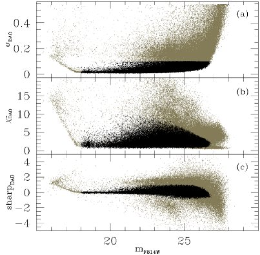
Figure 1: DAOPHOT photometric errors $\sigma_{DAO}$ (a), $\chi^{2}$ (b) and sharpness (c) plotted as a function of calibrated $m_{\rm F814W}$ magnitude (grey dots). The sources with $\sigma_{DAO}<0.1$ are indicated in the three plots with black dots.

The observations were designed as follows: images were obtained at three different pointing positions (covering an area of $200\arcsec\times 200\arcsec$ each) in the ${\rm F555W}$ and ${\rm F814W}$ filters (see Table 1). A single long exposure was centered on the nominal position of the cluster (central pointing). The other two pointings were spaced $\sim$1$\arcmin$ from the center of the cluster toward the North and toward the South, respectively. For both the northern and southern pointings a dither pattern was especially designed to allow for hot pixel removal, and to fill the gap between the two halves of the $4096\times 4096$ pixel detector. This dithering technique also improved both point–spread function (PSF) sampling and photometric accuracy by averaging the flat–field errors, and by smoothing over the spatial variations in detector response (see Table 1 and Fig. 1 in Paper I).

In addition, two short ($2-3\,\rm s$) exposures were obtained for both the northern and southern pointings, in the two filters, to recover the photometric information for the brightest sources.

All the images were taken with a gain of $2\,\rm e^{-}\,\rm{ADU}^{-1}$. The entire data set was processed adopting the standard STScI ACS calibration pipeline (CALACS) to subtract bias level, super-bias, and super-dark, and to apply the flat-field correction. For each filter, all the long exposures were co–added using the multidrizzle package (Koekemoer et al., 2002). This process also provided a correction for geometrical distortion. Cosmic rays (CRs) and hot pixels were removed. The data units were converted from electrons to electron–rates, and a final output image was obtained, sampled on a finer grid (the final pixel scale is $4/5$ of the original pixel dimension, equivalent to $0\farcs 039$). The pixel scale of the short exposures remained unchanged.

The final exposure time of the deep ${\rm F555W}$ and ${\rm F814W}$ images in the central region is $\simeq 4100\,\rm sec$ and the area is $\simeq 5\arcmin\times 5\arcmin$, corresponding to $\simeq 88\times 88\,\rm pc$.

2.2 Photometric reduction

The photometric reduction of the images has been performed with the DAOPHOT package within the IRAF environment.

We have followed the same methodology used for R136 (Sirianni et al., 2000) and NGC 330 (Sirianni et al., 2002), and used PSF fitting and aperture photometry routines provided within DAOPHOT to derive accurate photometry of all stars in the field. Given the different crowding properties of the long and the short exposures, we have performed PSF fitting photometry only on the mosaics obtained combining the long exposures, and aperture photometry on the images generated by the short exposures.

$\bullet$Short exposure photometry
First, we applied the automatic star detection routine DAOFIND to the ${\rm F555W}$ short mosaic to identify all the bright sources present in the image. In order to characterize the appropriate parameters that DAOFIND uses as selection criteria, we carefully selected by eye a sample of bona fide stars. We ran DAOFIND with a detection threshold set at $4\sigma$ above the local background level, and then we performed a visual inspection of the detected objects to reject features that had been misinterpreted as stars by the algorithm, such as spikes from saturated stars.

The stellar flux was measured in an aperture of $0\farcs 15$ radius, while the background was measured in an annulus located between $0\farcs 8$ and $0\farcs 9$ from the source peak.

The identification of the stars in the ${\rm F814W}$ short image was then forced assuming the final position of the stars detected in the ${\rm F555W}$ image.

Stars brighter than $m_{\rm F555W}<13$, and $m_{\rm F814W}<13$ are saturated. With the use of gain setting of 2 e^- ADU^-1, the WFC CCDs remain linear well beyond the physical saturation level (Gilliland, 2004). In order to recover some photometric information for the saturated stars, we performed aperture photometry on the saturated stars with an aperture of 10 pixels, following the procedure recommended by Sirianni et al. (2005).

The photometric calibration in the Vegamag system was performed by converting the magnitudes of the individual stars to an aperture radius of $0\farcs 5$ and by applying the zero–points listed in Sirianni et al. (2005). These are 25.724, and 25.501 for the filters ${\rm F555W}$ and ${\rm F814W}$, respectively.

$\bullet$Long exposure photometry
In the long exposures, stars were independently detected in each filter using the DAOFIND routine, with a detection threshold set at $4\sigma$ above the local background level. Their fluxes were measured by aperture photometry with an aperture of size $0\farcs 12$.

Because of the noticeable crowding in the long exposures, we performed PSF-fitting photometry to refine the photometric measurements of the individual sources.

In the ACS/WFC, the detector charge diffusion induces variations in core width and shape of PSF across the field of view (Krist, 2003; Sirianni et al., 2005). In order to take into account these variations it is necessary to compute a spatially variable PSF: 160 isolated and moderately bright stars, uniformly distributed over the entire image, were selected to properly sample the PSF. Stars brighter than $m_{\rm{F555W}}<18.0$, and $m_{\rm{F814W}}<18.0$ were discarded from the catalog, because of saturation. As for the short exposures, fluxes of individual stars were converted to an aperture of $0\farcs 5$ and appropriate zero–points were then applied. All the catalogs were cross-correlated and merged together. The final catalog contains the photometry obtained from both the short ($m_{\rm{F555W}}<18.0$ and $m_{\rm{F814W}}<18.4$) and long ($m_{\rm{F555W}}\gtrsim 18.0$, and $m_{\rm{F814W}}\gtrsim 18.4$) exposures. The final electronic catalog is shown in Table 2.

2.3 Photometric errors

For a safe interpretation of the characteristics of the observed stellar population, we need to distinguish true single stars from blended and/or residual spurious objects. Thus, we applied to our catalog selection criteria based on the quality of the photometric errors. Figure 1 shows the distributions of the DAOPHOT photometric errors ($\sigma_{\rm{DAO}}$), $\chi^{2}$ and sharpness as a function of the magnitude (grey dots) in the ${\rm F814W}$ filter. For each filter, we selected stars with $\sigma_{\rm{DAO}}<0.1$. We found that, once such a threshold on the DAOPHOT photometric error had been set, it was not necessary to apply further selection criteria, based e.g., on shape of the objects (as the sharpness), or on the ratio between the observed and the expected residuals obtained with the PSF-fitting (as the $\chi^{2}$ value).

In summary, 79,960 sources were found to have $\sigma_{\rm{DAO}}<0.1$ both in the ${\rm F555W}$ and ${\rm F814W}$ filters.

2.4 The CTE correction

All CCDs on the HST suffer a progressive degradation of their charge transfer efficiency (CTE) due to cosmic radiation, which causes the partial loss of signal when charges are transferred down the chip during the readout. The total amount of charge lost increases with the number of pixel transfers. CTE degradation can lead to photometric inaccuracy, since the position of a star on the chip may affect its recorded flux.

A parametric correction for the CTE losses for the WFC is published in the ACS Data Handbook (Pavlovsky et al., 2004). This photometric correction depends on the signal of the object, the background level, the number of charge transfers and the epoch of the observation.

This parameterization cannot be directly applied to our data, because, due to the complexity of our mosaic pattern (see Tab. 1), the same star lands in different positions in the different exposures, and, therefore, is subject to very different CTE effects. We, therefore, developed a special procedure (Sabbi, Sirianni & Nota, 2006).

First, for each filter, on each single exposure, previously corrected for geometric distortion, we performed aperture photometry with a radius of three pixels. The CTE parameterization, as described in the ACS Data Handbook, was then applied to each photometric catalog, taking into account the appropriate coordinate transformations, the exposure time, etc. All frames were aligned to the same coordinate system. Then, for each star in our final photometric catalog, we computed and applied an average CTE correction. The typical CTE correction applied to our data is $\sim$0.007 for the F555W filter, with a maximum value of $\sim$0.013 at $m_{\rm F555W}>26$, and $\sim$0.009 for the F814W filter, with a maximum value of $\sim$0.015 at $m_{\rm F814W}>25$.

A comparison between our F555W photometry and that obtained in the V band by Massey, Parker, & Garmany (1989) shows, on average, a difference of 0.03 magnitude, in agreement with the quoted errores between the two catalogs. We used Massey’s catalog also to determine the astrometric solution of our own catalog.

2.5 The Photometric Completeness

Artificial Star experiments are a standard procedure to test the level of completeness of photometric data. The experiment consists of adding onto a frame “artificial” stars obtained from the scaled PSF used in the photometric analysis of the frame. Then the artificial stars are retrieved. In total, more than 2,000,000 artificial stars were simultaneously simulated in the ${\rm F555W}$ and ${\rm F814W}$ deep exposures, and another 1,0000,000 were added to the short frames.

We used the sub–routine ADDSTAR in DAOPHOT to add the artificial stars; the routine inserts artificial stars of a user–specified magnitude in a copy of the original frame. We started from the ${\rm F555W}$ image. The artificial stars were distributed randomly in magnitude with a step function. This function extends two magnitudes below the detection limit of our observations, to probe with sufficient statistics the range of magnitude where incompleteness is expected to be most severe.

The most intriguing challenge of this experiment is to avoid that stars added artificially increase the crowding condition of the analyzed frame. To avoid this potentially serious bias, for both the short and long combined images, we have divided the ${\rm F555W}$ frame into a grid of sub–images of known width, and we have randomly positioned only one star in each sub–image. Each artificial star must have a distance from the sub–image edges large enough to guarantee that all its flux and background measuring regions fall within the sub–image, and thus do not contaminate the contiguous artificial star (see also Tosi et al., 2001). At each run, the absolute position of the grid with respect to the frame is randomly changed, guaranteeing that the artificial stars are uniformly distributed in coordinate space.

The frame where the artificial stars were added was reduced exactly as the original frame. We determined the level of completeness of the photometry by comparing the list of artificial stars added with the one of the stars recovered. We applied this procedure both to the deep and the short combined images.

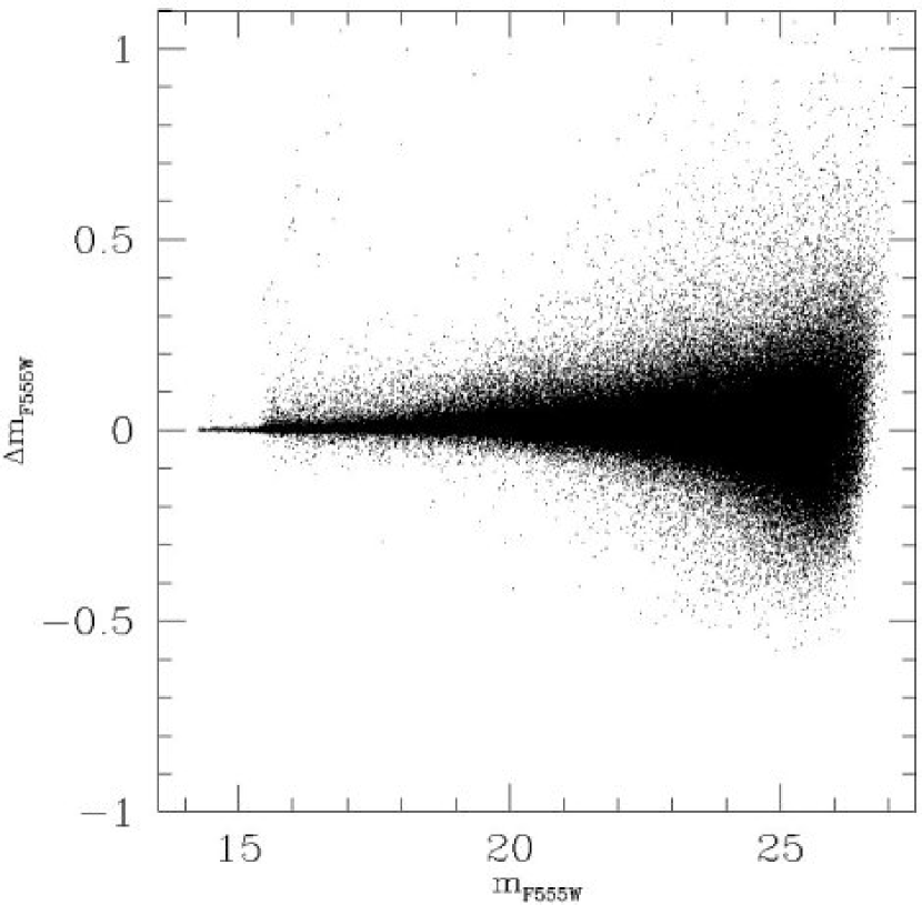
Figure 2: Diagram showing the $\Delta$ input-output magnitude as a function of input magnitude from the Artificial Stars experiments carried out on the ${\rm F555W}$ image, for artificial stars recovered with $\sigma_{DAO}<0.1$ in both filters.

In our experiment an artificial star is considered recovered if it is found in both frames with an input-output magnitude difference $\Delta m\leq 0.75$ (see Fig. 2), and at the same time satisfying all the photometric selection criteria (see § 2.3).

Figure 3 shows the completeness factor in each filter, defined as the percentage of the artificial stars successfully recovered compared with the total number of stars added to the data: the completeness is better than 50% down to $m_{\rm F555W}=25.19$ and $m_{\rm F814W}=23.57$.

3 The Color Magnitude Diagrams

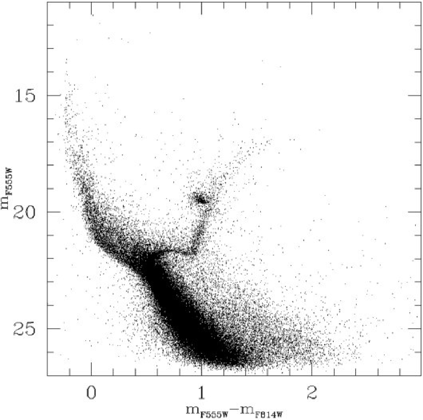
Figure 4: NGC 346 CMD $m_{\rm F555W}$ vs. $m_{\rm F555W}-m_{\rm F814}$ for all the stars with associated error smaller than 0.1 in both filters.

First results on the stellar content of NGC 346 were presented in Paper I. Figure 4 shows the $m_{\rm F555W}$ vs. $m_{\rm F555W}-m_{\rm F814W}$ Color–Magnitude diagram (CMD) of all the stars with $\sigma_{DAO}<0.1$ mag found in the combined frames. An electronic version of the photometric catalog is given in Table 2, which will be made available, and a subset of it is shown in this paper.

A first inspection of this CMD reveals that different stellar populations are present in the area:

$\bullet$ Young stars: A quite young stellar population is indicated by a bright ($12.5\lesssim m_{\rm F555W}\lesssim 22$) and blue ($-0.3\lesssim m_{\rm F555W}-m_{\rm F814W}\lesssim 0.4$) main sequence (MS), well visible to the upper left of the CMD.

A red ($1.5\lesssim m_{\rm F555W}-m_{\rm F814W}\lesssim 2.2$), faint ($m_{\rm F555W}\lesssim 21$) and well–populated sequence is also clearly visible in the faint and red part of the CMD. Stars in this region have colors and magnitudes consistent with being pre-MS stars in the mass range $0.6-3\,{\rm M}_{\odot}$, which were formed with the rest of the cluster (Paper I), $\sim 3-5\,{\rm Myr}$ ago.

$\bullet$ Intermediate and old age stars: An older stellar population is easily distinguishable in the CMD. Its rich MS extends from $m_{\rm F555W}\simeq 22$ down to $m_{\rm F555W}\simeq 26.5$. The evolved phases of this population are well delineated: a narrow sub giant branch (SGB) is visible at $m_{\rm F555W}\simeq 21.6$ between $0.45\lesssim m_{\rm F555W}-m_{\rm F814W}\lesssim 0.95$. A red giant branch (RGB) is very well defined with the brightest stars at $m_{\rm F555W}\simeq 17.3$ and $m_{\rm F555W}-m_{\rm F814W}\simeq 0.65$. The red clump (RC) of this population is visible at $m_{\rm F555W}\simeq 19.5$.

The relative thinness of the SGB suggests that the majority of the older stars in this field were formed in a single star formation episode that happened approximately $\sim$4–5 Gyr ago. In §4 we show that this result is due to the dominance of the star cluster BS90 over much of our field of view. The scattering of stars at fainter and brighter magnitudes than the cluster SGB indicates that star formation has occurred at earlier and later times in this direction.

$\bullet$ Comparison field: A SMC field ($\alpha=$ 00:58:42.5; $\delta=-$72:19:46) was observed with WFC for comparison. The observed field is located $\sim 9^{\prime}16^{\prime\prime}$ ($\sim 163\,{\rm pc}$ in projection) from NGC 346, and its $m_{\rm F555W}$ vs. $m_{\rm F555W}-m_{\rm F814W}$ CMD is shown in Figure 5. Only stars which in both filters have $\sigma_{DAO}<0.1$ are plotted. In this diagram we can clearly distinguish an old stellar population, characterized by broad SGB and RGB. Since the comparison field does not present any influence of the BS90 star cluster, we see clearer evidence for a wider range in ages and/or chemical abundances among the stars, possibly also mixed with more significant stellar population depth along the line of sight. Younger stars in the core helium burning blue loop phase are visible above the RC ($17\lesssim m_{\rm F555W}\lesssim 19$, $0.5\lesssim m_{\rm F555W}-m_{\rm F814W}\lesssim 1$) suggesting that star formation was recently active in this region.

Although a quantitative characterization of the field population will be possible only after computing synthetic CMDs, from the CMD morphology observed we can already infer that in this area a major episode of star formation occurred between 3 and 5 Gyr ago, but stars with ages up to at least 10 Gyr are also present. The MS of the field extends up to $m_{\rm F555W}\simeq 15$, but its brighter part is much less populated and less straight than that of NGC 346, indicating that at most recent epochs the SF activity in the field has been significantly lower, with a possible moderate enhancement $\sim 150\,{\rm Myr}$ ago.

3.1 Spatial distribution and age of the NGC 346 region stellar populations

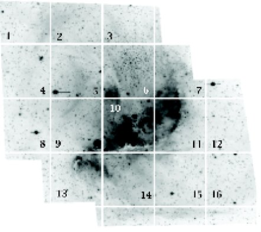
Figure 6: NGC 346 in the light of $\rm{F555W}$. The image was divided into 16 regions of $\simeq 0\farcm 3$ in size to study the spatial distribution of the various stellar populations.

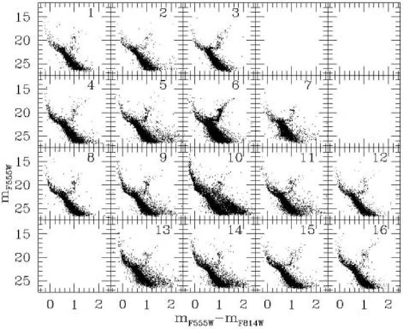
Figure 7: CMDs of the stars measured in the ACS FoV and selected on the basis of their position, indicated in Figure 6.

In order to investigate the spatial distribution of the identified stellar populations, we have divided the image in 16 regions of $\simeq 1\farcm 1\times 1\farcm 2$ in size, corresponding to $\simeq 19.4\times 21.2$ pc (see Fig 6). An inspection of the 16 CMDs covering nearly the entire region (Fig. 7) reveals that the spatial distribution of the various stellar populations is not uniform. Contamination from the SMC field also is observable at varying levels in all of the CMDs. We will analyze the Hess diagrams corrected for the field star populations in a later paper.

The diffuse nebulosity visible in Figure 1 in Paper I is due to the ionized gas contribution in H$\beta$ and [Oiii]. This is visible especially in regions 10 (which is at the center of the cluster), 11, and 13 (Southeast dusty region). In region 6, to the North of NGC 346, we clearly detect an increase of bright and red stars associated with the surprisingly rich BS90 star cluster (see §4) that was cataloged for the first time by Bica & Schmitt (1995).

The brightest ($m_{\rm F555W}\simeq 15.5$) and bluest ($m_{\rm F555W}-m_{\rm F814W}\simeq-0.2$) stars are concentrated in the CMD of region #10 (CMD–10) that corresponds to the center of NGC 346. This region is characterized by the presence of many bright and compact stellar sub–clusters, which will be further discussed in § 3.2. The brightest stars in this region have colors and magnitudes consistent with a stellar population of $3\pm 1$ Myr, and a mass of $\sim 50-60\,{\rm M}_{\odot}$. As in Paper I, this CMD shows also the largest number of candidate pre–MS stars ($\sim$2100 per unit area).

Candidate pre-MS stars are also visible, but in lower numbers, in the CMDs obtained for the regions around NGC 346 (regions 5, 6, 7, 9, 11, 13, 14, and 15). In particular CMD 11 (which corresponds to the region where we can see the dusty “ridge”) and CMD 13 (which corresponds to the region where the majority of embedded clusters are found, see §3.2 and Rubio et al., 2000) show a young MS nearly as bright ($m_{\rm F555W}\simeq 14-15$) as that in CMD 10, indicating that the star formation has been, and possibly still is, active in this region.

Region 6 is centered on the core of the star cluster BS90. The presence of this intermediate age stellar population is easily distinguishable in the corresponding CMD (CMD 6 in Fig. 7): compared with all the other CMDs, the old MS appears more populated ($\gtrsim 12100$ stars per unit area) and both the RGB and SGB are better delineated and narrower. The presence of this old stellar association is visible also in the surrounding regions (3, 5, 10, 11, and probably, 2, 7, 9).

CMD 4 corresponds to an external region located toward the East, at a distance of $\sim 141\arcsec$ ($\simeq 41.4$ pc) from the center. In this area the blue MS appears brighter ($m_{\rm F555W}\simeq 12.5$ in projection) than those of regions 1, 2 and 5, but pre–MS stars as young as those identified in the innermost CMDs are not present. The brightest and bluest stars detected in this area belong to a small stellar association, which is probably older, and likely not connected with NGC 346 (see § 3.2).

CMDs 1, 2, 8, 12, and 16, are at the outskirts of NGC 346, and show only the SMC field population (e.g. to be compared with the CMD in Fig. 5): in all these CMDs both the RGB and the SGB appear broader, and less well delineated than those observed in the innermost CMDs. Also the RC is less clearly defined. The blue MS in these CMDs ends at $m_{\rm F555W}\simeq 15$, as observed in the case of the comparison field.

We used the set of Padua isochrones (Bertelli et al., 1994), transformed into the VEGAMAG system by applying the transformations calculated by Origlia & Leitherer (2000), to derive a preliminary evaluation of the ages of the stellar populations identified. For this calculation we assumed a distance modulus $(m-M)_{0}=18.9$ and a Galactic foreground $E(B-V)=0.08$.

The blue MSs observed in the CMDs are likely to be the composition of multiple star formation episodes. In all the CMDs we found a young stellar population, belonging to the SMC field (see also Fig. 5). Superimposed on this population we found a $\sim 15\pm 2.5\,{\rm Myr}$ old stellar population in CMD 4, and a very young stellar population (with an age $\sim 3\pm 1$ Myr) in CMDs 5, 6, 7, 9, 10, 11, 13, 14, and 15. Similar age estimates are derived for the pre-MS candidates found in these CMDs.

3.2 The young stellar population

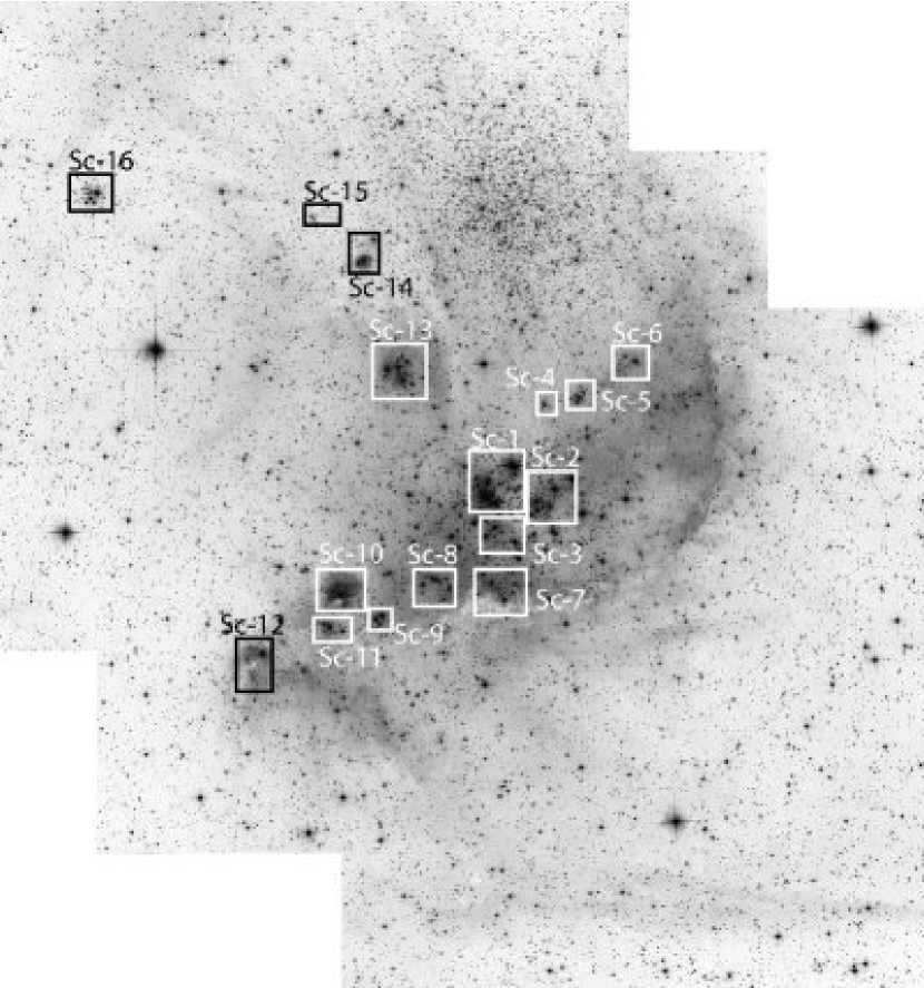
Figure 8: Stellar associations identified within the N66 nebula.

The youngest stellar population appears concentrated in a number of small compact stellar associations (see Fig. 8), which vary in density, dust content and morphology, and are co–located with the dense CO clumps found in the region by Rubio et al. (2000). The sub–clusters were first identified using isophotal contours; then we considered sub–clusters those stellar associations which show a stellar density at least three times higher than the average stellar density.

The majority of these associations are embedded in H II gas, whose distribution is traced (Fig. 8) by the diffuse emission in H$\beta$ and [Oiii] 4959, 5007.

In the deep HST/ACS images the central cluster seen in the ground based images is resolved in three separate sub–clusters (namely Sc–1, 2, and 3 in Fig. 8). Arcs of dust and gas depart from these three sub–clusters towards the Northwest and connect them with three smaller associations (Sc–4, 5, and 6).

Another 6 sub–clusters (namely Sc–7, 8, 9, 10, 11, and 12) are found toward the Southeast. Some of these associations (i.e. Sc–10, and 12) appear still embedded in dust and fuzzy nebulosities, and probably are sites of recent or even still ongoing star formation.

A dense clump of molecular gas is located along the perpendicular direction from the main body of NGC 346 to the Northeast (see Rubio et al., 2000). At its base there is another bright and dense sub–cluster (Sc–13). Another two faint and red associations (Sc–14, and 15 respectively), constituted almost exclusively by pre–MS stars, are located at the center of this clump.

Another bright sub–cluster (Sc–16) is located at the extreme Northeast periphery of the region. This association shows redder colors and does not display any nebulosity, suggesting an older age, with respect to the other younger star clusters.

The average characteristics of the sub–clusters are summarized in Table 3.

How did the star formation progress within the N66 nebula? Are all the stellar sub–clusters identified here coeval, or, as suggested by Massey, Parker, & Garmany (1989) did they form following a sequential process? Has N66 exhausted its fuel, or is its star formation still ongoing? If so where, and at what levels?

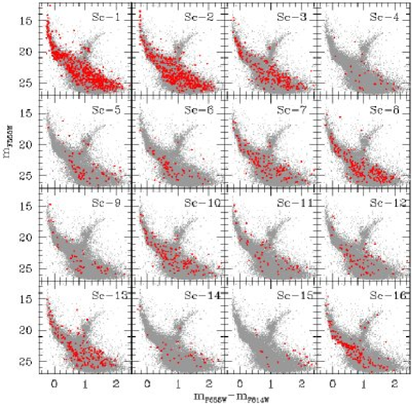
Figure 9: CMDs of the 16 sub–clusters identified within NGC 346 region. Red dots indicate stars within the sub–cluster radius (see Tab. 3). In order to better distinguish the evolutionary phases, sub–clusters CMDs are superimposed to the total CMD (grey dots).

The CMDs of all the young sub–clusters are shown in Figure 9. To estimate sub–clusters ages and determine how the star formation has progressed in the region, we fitted the CMDs of those sub–clusters which show a populated MS (Sc–1, 2, 3, 7, 8, 9, 10, 11, 13, and 16) with Padua isochrones (Bertelli et al., 1994). Because the majority of the sub–clusters populations are constituted by pre–MS stars, we used also pre-MS isochrones by Siess, Dufour & Forestini (2000), to evaluate the age of the various sub–clusters.

We found that:

• From the comparison with the Padua isochrones, we estimated an age of $3\pm 1\,{\rm Myr}$ for the MS of sub–clusters Sc–1, 2, 3 and 13. These 4 sub–clusters show also a high number of pre–MS stars (see Table 3). A comparison with Pre–MS isochrones (Siess, Dufour & Forestini, 2000), indicates ages of $4\pm 1\,{\rm Myr}$ for these stars. This is in good agreement with the age derived from the MS, taking into account that we are trying to estimate the age of the sub–clusters using different sets of isochrones, computed for different evolutionary phases.

• Compared to Sc–1, 2, 3, and 13, the MS of sub–clusters Sc–7, 8, 9, 10, and 11 appears redder, suggesting either that these sub–clusters are few million years older, or that they are coeval with the others, but affected by higher extinction. However, magnitudes and colors of the pre–MS stars in sub–clusters Sc–7, 8, and 10 appear too bright and red to be compatible with a stellar population older than $\sim 4\,{\rm Myr}$, indicating a more likely age of $3\pm 1\,{\rm Myr}$ also for these sub–clusters. This last hypothesis is also supported by the presence of dust and fuzzy nebulosities.

• Both MS and pre–MS isochrones indicate that the sub-cluster Sc–16 has an age of $15\pm 2.5\,{\rm Myr}$. It probably is a Pleiades-size open star cluster that may have formed independently of the main NGC 346 system.

• Figure 9 shows that sub–clusters Sc–5, 6, 12, 14, and 15 are not sufficiently populated to allow a statistically meaningful evaluation of their ages via MS fitting, but colors and magnitude of the pre–MS stars detected in these sub–clusters are in agreement with an age of $4\pm 1\,{\rm Myr}$.

The crossing time $T_{c}$ from the central sub–cluster to the external sub–clusters (namely Sc–6, 12, 15 and 16) for a sound speed of 10 Km/s is of order of $\sim 2\,{\rm Myr}$, with the exception of Sc–16 where it is $\simeq 4\,{\rm Myr}$.

Comparison with isochrones does not allow us to resolve differences in age smaller than 1–2 Myr. Within this margin, all sub–clusters appear coeval with each other. The one exception is Sc–16, that may not be related to the star-forming episode that originated NGC 346. The most massive and brightest stars are found in the three innermost clusters (namely Sc–1, 2, and 3). Moving from the center to the South the star clusters become progressively less massive. Star clusters towards the N, Northeast, are almost entirely constituted by low mass pre–MS stars, with only few stars, if any, on the MS. These sub–clusters are co–located with of the highest velocity CO clouds observed by Rubio et al. (2000); in particular Sc–14 and 15 are located in the center of the dense CO cloud in the Northeast “spur”.

The fact that the North, Northeast star clusters are co–located with the highest velocity CO clumps could indicate that the stellar winds have started to disperse the ionized gas on the North side of the nebula (Sc–4, 5, and 6). Towards the East and the South the gas density is likely high enough to resist the wind pressure. A multitude of dark Bok–globules, similar in structure to those in M 16 can be found close to the Southeast clusters, along a dust “ridge” which extends toward the South–Southwest. This suggests that N66 has not yet exhausted all its fuel, and that the star formation process is still active at some level in the periphery of the central cluster.

3.3 Star formation timing

The sequence of star formation in N66 presents an intriguing picture. Only Sc-16 appears to be old enough to be associated with the event that produced the larger SNRs in this region of the SMC (see §1). Ages of all of the other stellar groupings fall in the range of 2–5 Myr, implying an age spread, if present, of $\leq$3 Myr over an area that is about 40 pc in extent. The N66 region thus lies on the age spread–linear size relationship described by Elmegreen (2000).

Elmegreen (2000) interprets the age range-size correlation as a result of the formation of self-gravitating sub–clumps within 1–2 crossing times of a larger cloud complex. The observed sub–clusters in N66 then could be the products of the unstable sub–clumps required by this model, some of which may still be collapsing and are seen as the star forming CO-clouds. Following the discussion of Rubio et al. (2000), the diffuse molecular gas in the original cloud likely has been photodissociated and probably largely photoionized by O stars in the main NGC 346 cluster. The remaining molecular sub–clumps are experiencing rapid evolution due to photoevaporation from their surface PDRs and varying levels of star formation within the clouds.

In this conceptual model of the N66 region, most of the star formation was not triggered, but rather resulted from the turbulence driven density variations within a giant interstellar cloud complex. It also helps us understand how N66 can have a relatively normal structure which resembles Galactic Hii regions even when the mass loss rates from its O stars are substantially reduced relative to those of its Galactic counterparts (Bouret et al., 2003). Mechanical power from O-star winds is not a dominant factor in the evolution within N66. On the other hand the presence of multiple SNRs surrounding N66 (Reid et al., 2006) suggests that its outer could well be influenced by mechanical processes. We will return to a more detailed examination of relationships between stars and gas in a later paper.

4 BS90: A Rich Intermediate Age Star Cluster

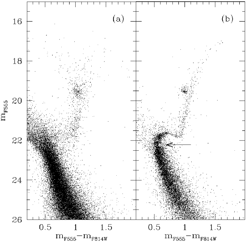
Figure 10: Comparison between the RGB of SMC field (a), that of the CMD #6, shown in Fig 7, corresponding to the intermediate–old age cluster (b). The black arrow in panel (b) highlights the position of the gap corresponding to the overall contraction of stars, when their central hydrogen fuel is consumed to a few percent.

As mentioned in § 3.1 an old stellar cluster is present in the region. It is clearly visible to the North of NGC 346 (see Fig. 1 in Paper I). Its CMD is displayed in Figure 10b. The various evolutionary features (MS, SGB, RGB and RC) are quite tight, showing that we are actually dealing with a simple stellar population. The quality of the photometry is such that we can clearly identify a horizontal gap at $m_{\rm F555W}\simeq 22.3$, just below the MS Turn–Off (TO). This gap corresponds to the overall contraction of stars when their central hydrogen fuel is consumed down to a few percent, and has been observed in Galactic open clusters of a few billion years (Bragaglia & Tosi, 2006, and references there in). The comparison of the cluster CMD with the Padua isochrones indicates that the system was formed around 4 Gyr ago. As noted in §3 the evolutionary sequences are wider in the field CMD (Fig. 10a) indicating that the field also developed a major episode of star formation between 3 and 5 Gyr ago, but it probably lasted longer. As a result, stars of different ages and metallicity are present.

We have seen in §3.2 that there is evidence of variable reddening in our data. Nevertheless both the RC and the SGB of the old star cluster do not seem to be affected by differential extinction, suggesting that the old cluster is likely placed in front of NGC 346.

In order to study the characteristics of this system we computed its density profile. First, we determined the center of gravity ($C_{\mathrm{grav}}$) of the stellar association, by estimating the position of the geometric center of the star distribution within an area of $\sim 4\arcmin\times 4\arcmin$ around the center of the cluster. To determine this position we applied the same procedure described in Montegriffo et al. (1995), which computes $C_{\mathrm{grav}}$ by simply averaging the $\alpha$ and $\delta$ coordinates of stars located in the selected area. The position we obtained for the stellar association is $\alpha=00^{h}59^{m}04\farcs 59,\,\delta=-72\arcdeg 09^{m}11\farcs 73\,[J2000]$, with a 1$\sigma$ uncertainty in both $\alpha$ and in $\delta$ of $\sim 0\farcs 5$, that corresponds to about 12 pixels in the HST/FWC images.

We computed the star density profile applying the standard procedure described in Calzetti et al. (1993): the entire photometric sample was divided into 15 concentric annuli, centered on $C_{grav}$, spanning a spatial range from $0\arcsec$ to $158\farcs 5$. Then, we determined the number of stars in each annulus. For each annulus the star density was obtained by dividing the number of stars by its area, expressed in arcsec².

Figure 11 shows the stellar density profile. The open triangles represent the density profile we obtain if we include all the stars present in our photometric catalog. The contamination due to the presence of NGC 346 is clearly visible. In order to reduce the sources of uncertainties we then re–computed the density profile considering only the stars redder than V$-$I$\gtrsim 0.4$. Stars bluer than this value belong to a young population, that can not be coeval, and thus related to the globular cluster. The candidate pre–MS stars were also removed from the catalog. The final density profile is also shown in Figure 11 (black dots). The error–bars were computed using the formula

$$\sigma=\sqrt{\frac{n_{\star,j}(1-n_{\star,j})}{A_{j}}}$$

were $n_{\star,j}$ is the number of stars within the j^th annulus, where $A_{j}$ is the area of the j^th annulus.

The solid line represents the best fit of the stellar density distribution of the old cluster (black dots), and was obtained by applying a King model (1966) with a core radius $r_{c}=25\arcsec$ and a tidal radius $r_{t}=130\arcsec$. The concentration of the cluster ($c=\log(r_{c}/r_{t})=0.72$) indicates that the cluster is still far from its gravitational collapse (see Meylan & Heggie, 1997), in agreement with its relatively young age ($\sim 4\,{\rm Gyr}$).

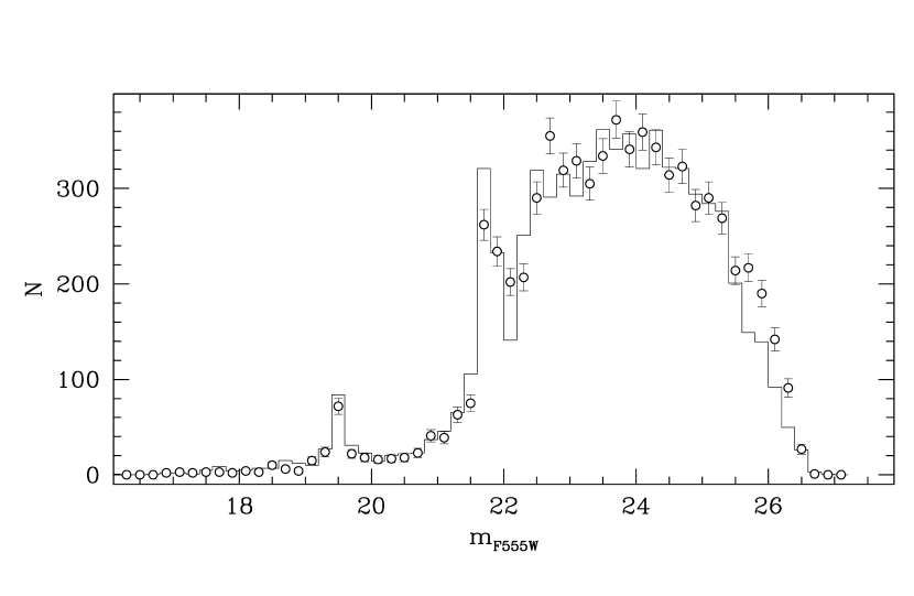
Figure 13: Comparison between the observed (open circles) and the synthetic (solid line) luminosity functions of the core of BS90.

To better estimate the age of the cluster, we applied the synthetic CMD method by Tosi et al. (1991) in the updated version described by Angeretti et al. (2005). We find that the synthetic model in better agreement with the data has Z=0.003, E(B-V)=0.08, distance modulus =18.9, age$=4.3\pm 0.1\,{\rm Gyr}$ and a fraction of binaries between 30 and 50%. The comparison between the observed and the synthetic CMDs of the core of the cluster is shown in Figure 12. Corresponding luminosity functions (LFs) are shown in Figure 13.

The circumstance that both the old cluster and the field contain a population $\simeq 4.3\,{\rm Gyr}$ old shows that in our observed region the star formation was quite active at that epoch. This result is not consistent with the simple two burst models proposed by Pagel & Tautvaisiene (1998) and Rich et al. (2000), but agrees with Gardiner & Hatzidimitriou (1992), Dolphin et al. (2001), and McCumber et al. (2005), who suggested that both the SMC field and the old star clusters have probably formed in a quasi–continuous mode with a broad peak between 4 and 12 Gyr.

The synthetic CMD methods allowed us also to estimate the entire mass content between $0.6\,{\rm M_{\odot}}$ and $120\,{\rm M}_{\odot}$ of the cluster within its core radius ($\sim$$5.6\times 10^{4}\,{\rm M}_{\odot}$). From the King profile, we estimated that this correspond to $\sim$77% of the total mass of the cluster. To take into account the contribution of the sources in the mass range between $0.05-0.6\,{\rm M}_{\odot}$, in this mass range, we have assumed an initial mass function with $\alpha=1.3$ (Kroupa & Weidner, 2003). In doing this we estimate for the cluster a total mass of $\sim$$1.03\times 10^{5}\,{\rm M}_{\odot}$.

5 Conclusions

Our analysis of the stellar content of N66/NGC 346 provides a snapshot of the star formation history of the entire region. From the analysis of the photometric data, we can conclude that different star formation episodes took place.

The oldest stellar population observed belongs to the SMC field. The morphology of the CMD suggests that, in the field, a major episode of SF occurred approximately between 3 and 5 Gyr ago, but stars with ages up to at least 10 Gyr are also present. We noted also that at most recent epochs the SF activity in the field has been significantly lower, with a possible moderate enhancement $\sim$150 Myr ago.

An intermediate–old age star cluster is located $\sim$23 pc in projection from the center of NGC 346. A comparison between the CMDs of this old cluster and that of the SMC field (see Fig. 10) indicates that the stars in the old association formed in an almost instantaneous burst of star formation $\sim$$4.3\pm 0.1\,{\rm Gyr}$ ago. The discovery of this intermediate–old age star cluster further supports the hypothesis suggested by Gardiner & Hatzidimitriou (1992), Dolphin et al. (2001), and McCumber et al. (2005) that, in the SMC, both the field and the star cluster populations have likely formed in a quasi–continuous mode.

The youngest stellar population belongs to NGC 346. Padua isochrones indicate that NGC 346 is $3\pm 1\,{\rm Myr}$ old. The MS of the youngest population abruptly interrupts at ${\rm F555W}\simeq 21$. At ${\rm F555W}>21$ we identify hundreds of stars whose colors and magnitude are consistent with those predicted for pre–MS stars (see also Paper I).

The high spatial resolution of our observations reveals that the youngest stellar population is not uniformly distributed within the ionized nebula: we identified at least 15 Sub–clusters, which differ in size and stellar content. Within the uncertainties due to the comparison with isochrones, the sub–clusters are likely coeval with each other (see Tab. 3). However a relatively older sub–cluster (Sc–16, with an age $15\pm 2.5\,{\rm Myr}$) is located at the Northeast periphery of our data. This sub–cluster is likely not related to the star forming episode that originated NGC 346.

Recent spectroscopic investigations of NGC 346 (Heap, Lanz, & Hubeny, 2006; Mokiem, 2006) confirm that the majority of the stars associated with the cluster have an age of 3 Myr, even if stars as young as 1 Myr are also present (but see the discussion in Massey et al., 2005). No relationship between the age of the stars and their distance from the cluster center is identified. Due to the age uncertainties quoted by the authors and the lower precision of the isochrones comparison technique, our results are in good agreement.

The sub–clusters coincide with the clumps of molecular gas identified by Rubio et al. (2000). Many of them, especially towards the Southeast, are close to obscure Bok–globules, which can contain still embedded Class I and 0 young stellar objects that would not be visible in the wavelength range covered by our data. The presence of diffuse gas and dust around these sub–clusters suggests that NGC 346 has likely not exhausted its fuel and star formation is possibly still ongoing.

All along the dust “ridge” of N66 it is possible to observe many dense nebular knots and dust pillars oriented toward the central clusters, that are similar in shape to those identified in 30 Doradus by Walborn, Maíz–Apellániz, & Barbá (2002). The presence of these structures strongly supports the hypothesis that the stellar winds, developed from the most massive stars in NGC 346, are probably triggering a secondary episode of star formation at the periphery of N66.

The most massive stars are located in the sub–clusters in the center of the nebula. We also find that sub–clusters located toward the North–Northeast are generally smaller and constituted mainly by pre–MS stars. These clusters coincide with the highest CO velocity clumps analyzed by Rubio et al. (2000). This seems to indicate that the UV radiation and the stellar winds from the stars in Sc–1, 2, and 3 are not isotropic, but they are more efficient in disrupting the molecular cloud toward the Northwest, making the star formation less efficient than toward the Southwest. Alternatively, it is possible that the interaction with SNR 0057–7233 is preventing the normal expansion of N66 along this direction.

NGC 346 is probably the result of the collapse and subsequent fragmentation of the initial giant molecular cloud in multiple “seeds” of star formation. The fact that the observed sub–clusters appear almost coeval, and that many of them appear to be connected by arcs of dust and gas, seems to be a good observational match to the conditions predicted by the hierarchical fragmentation of a turbulent molecular cloud model (Klessen & Burkert, 2000; Bonnell & Bate, 2002; Bonnell, Bate, & Vine, 2003).

According to this model the fragmentation of the cloud is due to supersonic turbulent motions present in the gas. The turbulence induces the formation of shocks in the gas, and produce filamentary structures (Bate, Bonnell, & Bromm, 2003). The chaotic nature of the turbulence increases locally the density in the filamentary structures. When regions of high density become self–gravitating, they start to collapse to form stars. Simulations show that star formation occur simultaneously at several different location in the cloud (Bonnell, Bate, & Vine, 2003), as appears to be the case for NGC 346.

Further UV and IR photometric and spectroscopic observations are necessary to better establish the mass and the ages of the stars, to verify if small differences in age are present among the sub–clusters, and to confirm the presence of ongoing star formation within N66. Furthermore, an analysis of the gas dynamics within N66 can confirm if the parent cloud underwent a hierarchical fragmentation: the formation of shocks in the gas, due to the initial supersonic turbulence, rapidly removes kinetic energy from the gas (Ostriker, Stone, & Gammie, 2001), and we expect to find very low gas velocities around the sub–clusters.

Figure 3: Completeness curves for the ${\rm F555W}$ (dashed line), and for the ${\rm F814W}$ (continuous line) photometry as a function of magnitude.

Figure 5: CMD of a SMC field region observed for comparison. The same error selection criteria used for NGC 346 were applied to this photometric catalog.

Figure 11: Observed radial density profile of the old cluster (black dots) and of the entire photometric catalog (open triangles), relative to the adopted $C_{grav}$. The solid line indicates the best-fit model ($r_{c}=25\arcsec$ and $c=0.72$) of the radial density distribution of the cluster.

Figure 12: Comparison between the observed (a) and the synthetic (b) CMDs for the core of BS90. The assumed fraction of binaries is 30%.

Table 1: Journal of WFC/ACS observations

Image Name	Filter	Exp. Time	R.A.	Dec.	Date	Flag
J92F01KRQ	${\rm F555W}$	003.0	$00^{\rm h}59^{\rm m}06\fs 72$	$-72\arcdeg 09\arcmin 40\farcs 3$	13 Jul 2004	N
J92F01KSQ	${\rm F555W}$	456.0	$00^{\rm h}59^{\rm m}06\fs 72$	$-72\arcdeg 09\arcmin 40\farcs 3$	13 Jul 2004	N
J92F01KUQ	${\rm F555W}$	456.0	$00^{\rm h}59^{\rm m}07\fs 02$	$-72\arcdeg 09\arcmin 40\farcs 1$	13 Jul 2004	N
J92F01KWQ	${\rm F555W}$	456.0	$00^{\rm h}59^{\rm m}07\fs 31$	$-72\arcdeg 09\arcmin 40\farcs 0$	13 Jul 2004	N
J92F01KYQ	${\rm F555W}$	456.0	$00^{\rm h}59^{\rm m}07\fs 61$	$-72\arcdeg 09\arcmin 39\farcs 8$	13 Jul 2004	N
J92F01L1Q	${\rm F555W}$	003.0	$00^{\rm h}59^{\rm m}06\fs 72$	$-72\arcdeg 09\arcmin 40\farcs 3$	13 Jul 2004	N
J92FA3VEQ	${\rm F555W}$	380.0	$00^{\rm h}59^{\rm m}06\fs 18$	$-72\arcdeg 10\arcmin 31\farcs 2$	15 Jul 2004	C
J92F02MBQ	${\rm F555W}$	003.0	$00^{\rm h}59^{\rm m}04\fs 68$	$-72\arcdeg 11\arcmin 21\farcs 7$	18 Jul 2004	S
J92F02MCQ	${\rm F555W}$	483.0	$00^{\rm h}59^{\rm m}05\fs 58$	$-72\arcdeg 11\arcmin 21\farcs 5$	18 Jul 2004	S
J92F02MEQ	${\rm F555W}$	483.0	$00^{\rm h}59^{\rm m}05\fs 28$	$-72\arcdeg 11\arcmin 21\farcs 6$	18 Jul 2004	S
J92F02MGQ	${\rm F555W}$	483.0	$00^{\rm h}59^{\rm m}04\fs 99$	$-72\arcdeg 11\arcmin 21\farcs 6$	18 Jul 2004	S
J92F02MIQ	${\rm F555W}$	483.0	$00^{\rm h}59^{\rm m}04\fs 68$	$-72\arcdeg 11\arcmin 21\farcs 7$	18 Jul 2004	S
J92F02MLQ	${\rm F555W}$	003.0	$00^{\rm h}59^{\rm m}04\fs 68$	$-72\arcdeg 11\arcmin 21\farcs 7$	18 Jul 2004	S
J92F01L3Q	${\rm F814W}$	002.0	$00^{\rm h}59^{\rm m}06\fs 72$	$-72\arcdeg 09\arcmin 40\farcs 3$	13 Jul 2004	N
J92F01L4Q	${\rm F814W}$	484.0	$00^{\rm h}59^{\rm m}06\fs 72$	$-72\arcdeg 09\arcmin 40\farcs 3$	13 Jul 2004	N
J92F01L6Q	${\rm F814W}$	484.0	$00^{\rm h}59^{\rm m}07\fs 02$	$-72\arcdeg 09\arcmin 40\farcs 1$	13 Jul 2004	N
J92F01L8Q	${\rm F814W}$	484.0	$00^{\rm h}59^{\rm m}07\fs 31$	$-72\arcdeg 09\arcmin 40\farcs 0$	13 Jul 2004	N
J92F01LAQ	${\rm F814W}$	484.0	$00^{\rm h}59^{\rm m}07\fs 61$	$-72\arcdeg 09\arcmin 39\farcs 8$	13 Jul 2004	N
J92F01LDQ	${\rm F814W}$	002.0	$00^{\rm h}59^{\rm m}06\fs 72$	$-72\arcdeg 09\arcmin 40\farcs 3$	13 Jul 2004	N
J92FA3VGQ	${\rm F814W}$	380.0	$00^{\rm h}59^{\rm m}06\fs 18$	$-72\arcdeg 10\arcmin 31\farcs 2$	15 Jul 2004	C
J92F02LUQ	${\rm F814W}$	002.0	$00^{\rm h}59^{\rm m}04\fs 68$	$-72\arcdeg 11\arcmin 21\farcs 7$	18 Jul 2004	S
J92F02LVQ	${\rm F814W}$	450.0	$00^{\rm h}59^{\rm m}05\fs 58$	$-72\arcdeg 11\arcmin 21\farcs 5$	18 Jul 2004	S
J92F02LYQ	${\rm F814W}$	450.0	$00^{\rm h}59^{\rm m}05\fs 28$	$-72\arcdeg 11\arcmin 21\farcs 6$	18 Jul 2004	S
J92F02M0Q	${\rm F814W}$	450.0	$00^{\rm h}59^{\rm m}04\fs 99$	$-72\arcdeg 11\arcmin 21\farcs 6$	18 Jul 2004	S
J92F02M5Q	${\rm F814W}$	450.0	$00^{\rm h}59^{\rm m}04\fs 68$	$-72\arcdeg 11\arcmin 21\farcs 7$	18 Jul 2004	S
J92F02M8Q	${\rm F814W}$	002.0	$00^{\rm h}59^{\rm m}04\fs 68$	$-72\arcdeg 11\arcmin 21\farcs 7$	18 Jul 2004	S

Table 2: Photometric catalog of the NGC 346 region. RA and Dec are in degrees. The electronic version of the table contains the entire list. This table is not included in this paper, but it will be made available upon publication.

ID	$m_{F555W}$	$\sigma_{F555W}$	$m_{F814W}$	$\sigma_{F814W}$	R.A.	Dec.	Reference
1	11.570	0.001	11.557	0.001	$0^{\rm h}59^{\rm m}26\fs 581$	$-72\arcdeg 09\arcmin 53\farcs 00$
2	11.916	0.001	11.841	0.001	$0^{\rm h}59^{\rm m}26\fs 571$	$-72\arcdeg 09\arcmin 53\farcs 99$
4	12.326	0.001	11.793	0.001	$0^{\rm h}58^{\rm m}42\fs 424$	$-72\arcdeg 09\arcmin 43\farcs 27$	MPG185
5	12.551	0.002	12.397	0.001	$0^{\rm h}59^{\rm m}31\fs 975$	$-72\arcdeg 10\arcmin 46\farcs 11$	MPG789
6	12.580	0.001	12.304	0.001	$0^{\rm h}59^{\rm m}26\fs 542$	$-72\arcdeg 09\arcmin 53\farcs 00$
7	12.609	0.002	12.742	0.002	$0^{\rm h}59^{\rm m}04\fs 479$	$-72\arcdeg 10\arcmin 24\farcs 77$	MPG435
8	12.734	0.002	12.398	0.001	$0^{\rm h}59^{\rm m}31\fs 975$	$-72\arcdeg 10\arcmin 46\farcs 13$
9	13.454	0.002	13.679	0.003	$0^{\rm h}59^{\rm m}00\fs 743$	$-72\arcdeg 10\arcmin 28\farcs 16$	MPG355
10	13.517	0.002	11.966	0.001	$0^{\rm h}58^{\rm m}53\fs 935$	$-72\arcdeg 12\arcmin 04\farcs 78$	MPG283

Table 3: Main characteristics of the NGC 346 sub–clusters

Sub–cluster	R.A.	Dec	radius	Age	total	PMS density
			parsec	Myr	# PMS	# PMS/parsec2
Sc–1	$00^{\rm h}59^{\rm m}05\fs 2$	$-72\arcdeg 10\arcmin 28$	2.5	$3\pm 1$	342	17.4
Sc–2	$00^{\rm h}59^{\rm m}01\fs 8$	$-72\arcdeg 10\arcmin 35$	2.3	$3\pm 1$	295	17.8
Sc–3	$00^{\rm h}59^{\rm m}06\fs 0$	$-72\arcdeg 10\arcmin 43$	1.6	$3\pm 1$	138	17.2
Sc–4	$00^{\rm h}59^{\rm m}02\fs 5$	$-72\arcdeg 10\arcmin 07$	0.6	$3\pm 1$	20	17.7
Sc–5	$00^{\rm h}59^{\rm m}00\fs 3$	$-72\arcdeg 10\arcmin 04$	1.1	$3\pm 1$	32	08.4
Sc–6	$00^{\rm h}58^{\rm m}57\fs 4$	$-72\arcdeg 09\arcmin 55$	1.2	$3\pm 1$	14	03.1
Sc–7	$00^{\rm h}59^{\rm m}05\fs 4$	$-72\arcdeg 10\arcmin 57$	1.5	$3\pm 1$	65	09.2
Sc–8	$00^{\rm h}59^{\rm m}07\fs 7$	$-72\arcdeg 10\arcmin 48$	1.9	$3\pm 1$	109	09.6
Sc–9	$00^{\rm h}59^{\rm m}12\fs 5$	$-72\arcdeg 11\arcmin 08$	1.0	$3\pm 1$	29	09.2
Sc–10	$00^{\rm h}59^{\rm m}14\fs 9$	$-72\arcdeg 11\arcmin 01$	1.6	$3\pm 1$	61	07.6
Sc–11	$00^{\rm h}59^{\rm m}15\fs 3$	$-72\arcdeg 11\arcmin 12$	1.1	$3\pm 1$	38	10.0
Sc–12	$00^{\rm h}59^{\rm m}19\fs 8$	$-72\arcdeg 11\arcmin 20$	1.5	$3\pm 1$	25	03.5
Sc–13	$00^{\rm h}59^{\rm m}11\fs 3$	$-72\arcdeg 10\arcmin 00$	1.9	$3\pm 1$	90	07.9
Sc–14	$00^{\rm h}59^{\rm m}13\fs 9$	$-72\arcdeg 09\arcmin 27$	0.9	$3\pm 1$	22	08.6
Sc–15	$00^{\rm h}59^{\rm m}17\fs 0$	$-72\arcdeg 09\arcmin 15$	0.6	$3\pm 1$	21	18.6
Sc–16	$00^{\rm h}59^{\rm m}30\fs 8$	$-72\arcdeg 09\arcmin 10$	1.6	$15\pm 2.5$	65	08.0

References

- Angeretti et al. (2005) Angeretti, L., Tosi, M., Greggio, L., Sabbi, E., Aloisi, A., & Leitherer, C. 2005, AJ, 129, 2203
- Bate, Bonnell, & Bromm (2003) Bate, M.R., Bonnell, I.A., & Bromm, V. 2003, MNRAS, 339, 577
- Bica & Schmitt (1995) Bica, E.L.D., & Scmitt, H.R. 1995 ApJS, 101, 41
- Bertelli et al. (1994) Bertelli, G., Bressan, A., Chiosi, C. Fagotto, F., & Nasi, E. 1994, A&AS, 106, 275
- Bragaglia & Tosi (2006) Bragaglia, A., Tosi, M. 2006, AJ, 131, 1544
- Bonnell & Bate (2002) Bonnell, I.A., & Bate, M.R. 2002, MNRAS, 336, 659
- Bonnell, Bate, & Vine (2003) Bonnell, I.A., Bate, M.R., & Vine, S.G. 2003, MNRAS, 343, 413
- Bouret et al. (2003) Bouret, J.C., Lanz, T., Hillier, D.J., Heap, S.R., Hubeny, I., Lennon, D. J., Smith, L.J., & Evans, C.J. 2003, ApJ, 595, 1182
- Calzetti et al. (1993) Calzetti, D., de Marchi, G., Paresce, F., & Shara, M. 1993, ApJ, 402, 1
- Chabrier (2005) Chabrier, G. 2005, in “The initial mass function 50 years later”, 41, E. Corelli, F. Palla, & H. Zinnecker eds, 2005, ASS library 327, Springer
- Danforth et al. (2003) Danforth, C.W., Sankirt, R., Blair, W.P., Howk, J.C., & Chu, Y.H. 2003, ApJ, 586, 1179
- Dolphin et al. (2001) Dolphin, A.E., Walker, A.R., Hodge, P.W., Mateo, M., Olszewski, E.W., Schommer, R.A. & Suntzeff, N.B. 2001 ApJ, 562, 303
- Elmegreen (2000) Elmegreen, B.G. 2000, AJ, 530, 227
- Fagotto et al. (1994a) Fagotto, F., Bressan, A., Bertelli, G., & Chiosi, C. 1994a, A&AS, 104, 365
- Fagotto et al. (1994b) Fagotto, F., Bressan, A., Bertelli, G., & Chiosi, C. 1994b, A&AS, 105, 29
- Gardiner & Hatzidimitriou (1992) Gardiner, L.T., Hatzidimitriou, D. 1992, MNRAS, 257, 195
- Gilliland (2004) Gilliland. R.L. 2004, Instrument Science Report ACS 04–01, (Baltimore, MD: STScI)
- Haser et al. (1998) Haser, S.M., Pauldrach, A.W.A., Leonnon, D.J., Kudrizki, R.–P., Lennon, M., Puls, J., & Voels, S.A. 1998, A&A, 330, 285
- Heap, Lanz, & Hubeny (2006) Heap, S., Lanz, T., & Hubeny, I. 2006, ApJ, 638, 409
- Hilditch, Howarth & Harries (2005) Hilditch, R.W., Howarth, I.D., & Harries, T.J. 2005, MNRAS, 125, 336
- Hoopes et al. (2002) Hoopes, C.G., Sembach, K.R., Howk, J.C., Savage, B.D., & Fullerton, A.W. 2002, ApJ, 569, 233
- Izotov, Thuan, & Lipovetsky (1997) Izotov, Y.I., Thuan, T.X., & Lipovetsky, V.A 1997, ApJS, 108, 1
- Izotov & Thuan (1999) Izotov, Y.I., & Thuan, T.X. 1999, ApJ, 511, 639
- King (1966) King, I.R. 1966, AJ, 71, 75
- Klessen & Burkert (2000) Klessen, R.S., Burkert, A. 2000, ApJS, 128, 287
- Koekemoer et al. (2002) Koekemoer, A.M., Fruchter, A.S., Hook, R, & Hack, W. 2002, in Proc 2002 HST Calibration Workshop, eds. S. Arribas, A. Koekemoer, & B. Whitmore (STScI: Baltimore, MD), 337
- Koeningsberger, Kuruckz, & Georgiev (2002) Koeningsberger,G., Kuruckz, R.L., & Georgiev, L. 2002, ApJ, 581, 598
- Krist (2003) Krist, J.E., 2003 ACS Instrument Science Report 2003–06, STScI
- Kroupa & Weidner (2003) Kroupa, P., & Weidner, C. 2003, ApJ, 598, 1076
- Massey, Parker, & Garmany (1989) Massey, P., Parker, J.W., & Garmany, C.D. 1989, AJ, 94, 1305
- Massey et al. (2005) Massey, P., Puls, J., Pauldrach, A.W.A., Bresolin, F., Kudritzki, R.P., Simon, T. 2005, ApJ, 627, 477
- McCumber et al. (2005) McCumber, M.P., Garnett, D.R., Dufour, R.J. 2005, AJ, 130, 108
- Mokiem (2006) Mokiem, M.R. 2006, “The physical properties of early–type massive stars (Ph.D. Thesys)
- Nazè et al. (2002) Nazè, Y., Hartwell, J.M., Stevens, J.R., Corcoran, M.F., Koeningsberger, G., Moffat, A.F.J., & Niemela, V.S. 2002, ApJ, 580, 225
- Nazè et al. (2003) Nazè, Y., Hartwell, J.M., Stevens, J.R.,Manford, J., Marchenko, S., Corcoran, M.F., Moffat, A.F.J.,& Skalkowski, G. 2003, ApJ, 586, 983
- Niemela, Marraco, & Cabanne (1986) Niemela, V.S., Marraco, H.G., & Cabanne, M.L. 1986, PASP, 98, 1133
- Nota et al. (2006) Nota, A., Sirianni, M., Sabbi, E., Tosi, M., Meixner, M., Gallagher, J., Clampin, M., Oey, S., Smith, L.J., Walterbos, R., & Mack, J. 2006, ApJ, 640, 29 (Paper I)
- Olive, Skillman, & Steigman (1997) Olive, K.A., Skillman, E., & Steigman, G. 1997, ApJ, 483, 788
- Origlia & Leitherer (2000) Origlia, L. & Leitherer, C. 2000, AJ, 119, 2018
- Ostriker, Stone, & Gammie (2001) Ostriker, E.C., Stone, J.M., & Gammie, C.F. 2001, ApJ, 546, 980
- Pagel & Tautvaisiene (1998) Pagel, B.E.J, & Tautvaisiene, G. 1998, MNRAS, 299, 535
- Pavlovsky et al. (2004a) Pavlovsky C., et al. 2004, “ACS Instrument Handbook”, Version 5.0, (Baltimore: STScI)
- Pavlovsky et al. (2004) Pavlovsky, C., Reiss, A., Mack, J., & Gilliland, R. 2004, “ACS Data Handbook”, Version 3.0, (Baltimore: STScI)
- Peimbert, Peimbert, & Ruiz (2000) Peimbert, M., Peimbert, A., & Ruiz, M.T. 2000, ApJ, 541, 688
- Peimbert, Peimbert, & Luridiana (2002) Peimbert, M., Peimbert, A., & Luridiana V. 2002, ApJ, 565, 668
- Reid et al. (2006) Reid, W. A., Payne, J. L., Filipović, M. D., Danforth, C. W., Jones, P. A., White, G. L., & Stavely-Smith, L. 2006, MNRAS, 367, 1393
- Relaño, Peimbert, & Beckman (2002) Relaño, M., Peimbert, M., & Beckman, J. 2002, ApJ, 564, 704
- Rich et al. (2000) Rich, R.M., Shara, M., Fall, S.M, Zurek, D.2000, AJ, 119, 197
- Rubio et al. (2000) Rubio, M., Contursi, A., Lequeux, J., Probst, R., Barbà, R.H., Boulanger, F., Cesarsky, D., & Maoli, R. 2000, A&A, 359, 1139
- Sabbi, Sirianni & Nota (2006) Sabbi, E., Sirianni, M., & Nota, A. 2006, “The 2005 HST Calibration Workshop, Hubble After the Transition to Two–Gyro Mode”, ed Koekemoer, Goudfrooij & Dressel, 41
- Siess, Dufour & Forestini (2000) Siess, L., Dufour, E., & Forestini, M. 2000, A&A, 358, 593
- Sirianni et al. (2000) Sirianni, M., Nota, A., De Marchi, G., Leitherer, C., & Clampin, M. 2000, ApJ, 579, 288
- Sirianni et al. (2002) Sirianni, M., Nota, A., Leitherer, C., De Marchi, G., & Clampin, M. 2000, ApJ, 533, 203
- Sirianni et al. (2005) Sirianni, M., et al. 2005, PASP, 117, 1049
- Tosi et al. (1991) Tosi, M., Greggio, L., Marconi, G., & Focardi, P. 1991, AJ, 102, 951
- Tosi et al. (2001) Tosi, M., Sabbi, E., Bellazzini, M., Aloisi, A., Greggio, L., Leitherer, C., & Montegriffo, P. 2001, AJ, 122, 1271
- Walborn (1978) Walborn, N.R. 1978, ApJ, 224L, 133
- Walborn & Blades (1986) Walborn, N.R., & Blades, J.C. 1986, ApJ, 304, 17
- Walborn & Parker (1992) Walborn, N.R., & Parker, J.W. 1992, ApJ, 399, 87
- Walborn, Maíz–Apellániz, & Barbá (2002) Walborn, N.R., Maíz–Apellániz, J.,& Barbá, R.H. 2002, AJ, 124, 1601
- Ye, Turtle, & Kennicutt (1991) Ye, T., Turtle, A.J., & Kennicutt, R.C.Jr. 1991, MNRAS, 249, 722