A Canis Major over-density imaging survey. I. Stellar content and star-count maps:
A distinctly elongated body of main sequence stars

Abstract

We present first results from a large-area ($\sim$80^∘$\times$20^∘), sparsely sampled two-filter (B,R) imaging survey towards the Canis Major stellar over-density, claimed to be a disrupting Milky Way satellite galaxy. Utilizing stellar colour-magnitude diagrams reaching to B$\sim$22 mag, we provide a first delineation of its surface density distribution using main sequence stars. It is located below the Galactic mid-plane, and can be discerned to at least b=-15^∘. Its projected shape is highly elongated, nearly parallel to the Galactic plane, with an axis ratio of $\gtrsim$ 5:1, substantially more so than what Martin et al. originally found. We also provide a first map of a prominent over-density of blue, presumably younger main sequence stars, which appears to have a maximum near [l,b $\sim$ 240^∘, -7^∘ ] and extends in latitude to b$\sim$ -10^∘. The young population is markedly more localized. We estimate an upper limit on the line-of-sight depth, $\sigma_{\rm los}$, of the old population based on the main sequence width, by comparing with a simple stellar population (Pal 12), obtaining $\sigma_{\rm los}$ $<$ 1.8 $\pm$ 0.3 kpc, at an adopted D_⊙ = 7.5 $\pm$ 1 kpc. For the young stellar population, we find $\sigma_{\rm los}$ $<$ 1.5 kpc. The overall picture presented is one of a young stellar population that is less extended, both in terms its line-of-sight depth and angular size, than the older population. In the literature three explanations for the CMa over-density have been invoked, namely (a) a partially disrupting dwarf galaxy on a low-latitude orbit, (b) a projection of a warped outer Galactic disk, and (c) a projection of an out-of-plane spiral arm. While the data provide no firm arguments against the less well-defined third scenario, they have clear implications for each of the others: (a) We infer from the strong elongation of the over-density in longitude, and simulations in the literature, that the CMa over-density is unlikely to be a gravitationally bound system at the present epoch, but may well be just a recently disrupted satellite remnant. A complexity for the satellite origin may arise from the ‘flattening’ of the young MS population, which is possibly more pronounced than the older one. (b) Based on modeling, we find that the line-of-sight depth of the MS over-density in old stars is clearly inconsistent with published locally axi-symmetric descriptions of the warped Galactic disk, such as those considered in Momany et al. (2006). Without detailed modeling, the data-set itself does not provide sufficient leverage to distinguish between an interpretation as sub-structure in the warped outer Galactic disk or a disrupted satellite.

1. Introduction

The current paradigm in which large disk galaxies like our Milky Way form (e.g. White & Rees 1978; White & Frenk 1991), is based on the successive coalescence and accretion of smaller systems of dark matter, stars, and diffuse interstellar gas into larger assemblies. Some of these smaller systems may be satellite dwarf galaxies that can be disrupted by tidal shocks and evaporation in a Galactic potential, and can spawn tidal tails. Numerical simulations exist that model distinct tidal stellar streams in and around large galaxies, indicating that at r$\gtrsim 10$kpc such streams should remain detectable as coherent stellar over-densities for billions of years (Johnston et al. 1999; Ibata & Lewis 1998; Martínez-Delgado et al. 2004; Peñarrubia et al. 2006).

Recently, much work has focused on a possible low-latitude stellar stream, the so-called Monoceros stream, encircling the Milky Way (MW) at a galacto-centric distance of around 20 kpc, which was found through colour-magnitude diagrams (CMDs) from SDSS (Newberg et al. 2002; Yanny et al. 2003); also see Ibata et al. (2003), Conn et al. (2005) & Martin et al. (2006). For stellar over-densities at low galactic latitudes it is not obvious a priori whether such a stream is of external origin, i.e. the tidal debris of a now (partially) disrupted satellite or, alternatively, a distorted part of the pre-existing outer stellar disk.

Arguments in favour of the dwarf satellite hypothesis have come from dynamical modeling (Peñarrubia et al. 2005), showing that it is possible to find a plausible model of the Monoceros stream that explains all detected parts of this low-latitude stream as the wrapped tidal debris tails of a disrupting (model) dwarf galaxy. In this dynamical model the position of the CMa over-density is not an initial constraint, and yet the main body of the disrupting model satellite happens to located in the direction of CMa at the present epoch. All kinematics, including the subsequently determined proper motion (Dinescu et al. 2005) of main sequence (MS) stars in a small area (0.25 deg²) towards the CMa stellar over-density are consistent with the dynamical model. Additional empirical support appears to come from the apparent bifurcation of suspected Monoceros stream stars at right ascension $\sim$ 120^∘ in Fig.1 of Belokurov et al. (2006), as could be expected in general based on the above-mentioned Peñarrubia et al. model. Other evidence comes from the discovery of an over-density of possible Monoceros stream RR Lyrae stars (Vivas et al. 2006), whose distances closely match the model expectation in Peñarrubia et al. (2005).

The position and survival of the progenitor of this stellar stream is still under debate. The best candidate is a seemingly well-defined stellar over-density of stars discovered in the direction of Canis Major (CMa) using 2MASS red giants (Martin et al. 2004a). This discovery has spawned a lively debate in the literature on whether this apparent over-density of red giants could be part of the distorted outer stellar disk (Momany et al. 2004; 2006; see also Rocha-Pinto et al. 2006) or an accreted and possibly disrupting satellite [Martin et al. 2004b; Martinez-Delgado et al 2005 (MD05); Bellazzini et al. 2006 (B06)]. However, a firm large-area kinematical, spatial and chemical link between the three known stellar components of the overall debate (i.e. the young and old stellar over-densities, and the Monoceros stream) is lacking.

From deep, visible-band photometry there are signs of at least two different star formation episodes in the direction of CMa [Bellazzini et al. (2005), B05; MD05; Carraro et al. (2005)]. For the sake of clarity, we illustrate this in an annotated colour-magnitude diagram, Fig. 1, which corresponds to a field near the presumed centre of the CMa over-density, and where the data are taken from this survey (see Sec. 2). Whether the most recent burst of star formation activity occurred 1-2 Gyr ago, as touted in B05, has been debated, in favour of a much younger stellar population of $\lesssim$ 100 Myr-old stars (Carraro et al. 2005). The CMa over-density itself, which is taken to lie near D_⊙=7.5 kpc (B05,MD05), comprises a predominantly older population of stars (4-10 Gyr; B05) and Moitinho et al. (2006) suggest that it may be consequence of viewing a local arm-like MW stellar sub-structure in projection. For a different and independent study of the stellar populations, we will make use of detailed CMD-fitting in a forth-coming paper (de Jong et al., in prep.).

To determine the full angular extent of the young and old main sequence stars towards CMa and to test whether they stem from a satellite galaxy, we conducted a large-area ($\sim$80^∘$\times$20^∘), sparsely sampled visible-band imaging survey of the CMa region, drawing on the wide field imager (WFI) at the MPG/ESO 2.2 m telescope on La Silla. The survey sub-area considered in this paper is 230^∘ $\lesssim$ l $\lesssim$ 260^∘, -20^∘ $\lesssim$ b $\lesssim$ 15^∘.

1.1. Aim and design of the WFI survey

The principal goal of our imaging survey is to provide a database that can address ultimately whether the CMa stellar over-density results from a dynamical distortion of the outer Galactic disk or whether it is the remains of a formerly large dwarf galaxy. As a step towards this goal, we aim to map its full angular extent through its star-count profile.

Recent reports (B06) based on 2MASS red clump stars suggest that the discernable part of the CMa over-density may extend across several 100deg² on the sky. Our survey goal is to cover this over-density through sparse sampling, but with relatively deep visible-band imaging. Specifically, we want to obtain CMDs that reach well below the turn-off magnitude of an ancient stellar population; our target limiting magnitude is B, R = 23 mag (S/N = 10). We chose a wide colour baseline (B-R) to have sensitivity to age- and/ or [Fe/H]-dependent CMD features (young MS, old MS turn-off and the red clump). The key difference (and merit) of the present CMa survey over previous large-area surveys, which have been based exclusively on 2MASS red-giant stars and MW models, is that we base our analysis on colour-magnitude diagrams that exhibit a well-defined stellar main sequence at a defined distance range. This provides an independent and high-contrast way of tracing the full angular extent of the CMa over-density. The chief disadvantage of visible-band data is that Galactic extinction in many parts of this area is high, A_V$\gtrsim$0.5 mag.

1.2. Aim of this paper

In this paper we present the data from the first observing phase of our imaging survey, covering the region around [l,b = 240^∘, -8^∘] that had originally been identified as the over-density in Martin et al. (2004a). As it turns-out, these data provide only partial spatial coverage of the over-density. Therefore, we refrain from a wide-spread quantitative comparison with Galaxy star-count models, except (i) to use a Besancon model CMD as a visual guide for the reader to help interpret the general morphology in our control CMDs, and (ii) to aid the discussion in Sec. 7.2.

We report our observations, and present the data and their reduction in Sec. 2. The issue of photometry completeness and uncertainties is assessed in Sec. 2.1. The crucial issue of reddening by dust extinction and its correction is presented in Sec. 2.2. In Sec. 3, we explain the choice of control fields, which is followed by a description of the stellar content and morphology of the CMDs in Sec. 4. In Sec. 5 we provide a star-count analysis of young and old CMa main sequence stars. We estimate an upper limit on the line-of-sight size of the CMa stellar overdensity in Sec. 6. We briefly discuss our results in Sec. 7 and summarize the key results in Sec. 8.

2. Observations, data and data reduction

All observations were carried out in service mode with the wide-field imager (WFI) on the 2.2-m ESO/MPG telescope at the La Silla observatory (Chile) from December 9 to 20, 2004. The WFI’s field-of-view covers 0.25 deg², sampled at 0.238^′′ pixel^-1. Single exposure images were taken in the B- and R-bands, at 100 s per pointing and filter. A total of 59 pointings (Table 1) provides a sparse map of the stellar over-density region originally identified in Martin et al. (2004a). B- and R-band pointings typically differ by less than 2.5 arcsec, which leads to negligible field-to-field differences in the (effective) imaging area. Overscan, bias, flat-field corrections, and an astrometric correction were performed using a pre-reduction pipeline (Schirmer et al. 2003). We obtained stellar photometry using DAOPHOT tools, available in IRAF. For each WFI pointing, we employed point spread function (PSF)-fitting using a spatially variable (order 2) moffat function of exponent 2.5, derived from 100 stars. The DAOPHOT/ALLSTAR PSF-fitting task is run on each frame separately. As we have single exposures per pointing, cosmic rays are effectively filtered out during the PSF-fitting and the matching of the B- and R-band photometry lists. Objects in each list are then assigned Galactic coordinates and are matched using a separation tolerance of 1.7 arcsec. This large tolerance ensures that the faintest stars, which have the poorest positional errors, are matched; and is tolerable owing to the sparseness of the fields surveyed.

For the photometric zero-points, we firstly tie the photometry from each observing night to a common internal (i.e. instrumental) zero point using the zero-point of each PSF (computed from its flux and magnitude). This is followed by the transformation of the instrumental magnitudes into the standard Johnson-Cousins photometric system based on observations of either standard stars from Landolt (1992) [for Dec. 17, 18] or secondary standards from Galadi-Enriquez et al. (2000) [on Dec. 20.] or both [Dec. 9], taken before or after our observations. For all standard star observations, atmospheric conditions were photometric. The calibration photometry, obtained from large (r=2.1 arcsec) circular apertures, is used to transform our instrumental magnitudes (b, r) into the Johnson-Cousins standard system (B,R). We estimate the colour terms (see Eqns. 1 and  2.) using 20 calibration stars from Dec. 9 with standard colours (B-R) in the range $\sim$ 0.8 to 1.6 mag. While we do not have enough calibration stars to determine accurate colour terms for each night separately, CMa observations were always performed under photometrically clear conditions, and so we use the colour terms from Dec. 9 for each of the observations. For a determination of the photometric zero-point offset(s), we have 4 to 20 calibration stars each night, except for Dec. 15 & 16., for which the calibration from Dec. 18 is used. With the instrumental fluxes already scaled to photons per second, the transformation equations for Dec. 18, for example, are

$$B=-b+24.86(\pm 0.01)+0.17(\pm 0.01)\,(B-R)$$ (1)

$$R=-r+24.48(\pm 0.04)-0.07(\pm 0.03)\,(B-R)$$ (2)

where the instrumental magnitudes (b,r) are corrected for atmospheric extinction. We adopted the atmospheric extinction co-efficients given in the ESO/WFI web-pages; those are 0.24 and 0.09 for the B- and R-bands respectively. The error values given in Eqns. 1 and  2 are the rms uncertainties.

The survey photometry is filtered using quality-control parameters computed by ALLSTAR in DAOPHOT, retaining only stars with acceptable CHI and SHARP parameters as well as formal magnitude errors $\sigma_{\rm B}<$ 0.15 mag and $\sigma_{\rm R}<$ 0.15 mag. Galactic coordinates and the number of selected stars per field is given in Table 1.

2.1. Completeness and photometry errors

To assess the point-source completeness, we performed artificial star tests for a representative set of six fields. Specifically, we added a total of several thousand stars, in groups of 1300, in the (instrumental) magnitude range 15.5 to 25.5 mag, to each image. The fake stars that we added at random locations to these largely uncrowded fields increase the number-density by up to 10%, hence barely altering crowding effects. Stars injected in the B- and R-band images did not have the same locations. We then determined the completeness fractions, defined as the ratio of recovered artificial stars to the number of the injected ones, at 0.75 mag-wide intervals. We brighten the B- and R- fake star magnitudes by 0.42 and 0.13 mag, respectively, to shift them approximately from instrumental magnitudes to the flux-calibrated magnitude scale. Also, as we use de-reddened CMDs in this paper, we shift the the magnitude scale of the completeness curves accordingly and denote the shifted B- and R-band magnitudes by B^′ and R^′ respectively in Fig. 2. The completeness at (l,b) = (241.5^∘,-6^∘) is above 90% for B^′ or R^′ $\lesssim$ 20.6 mag (see Fig. 2). In the matched B- and R-band photometry lists the completeness is less, and is typically above $\sim$ 80% at B^′ $\lesssim$ 20.6 mag. This 80% completeness limit varies by $\pm$ $\sim$ 0.5 mag across the area surveyed at $|$b$|$$\gtrsim$6^∘.

The completeness at each pointing is reduced by gaps between detector chips, bad columns and pixels that are the same for each field. Completeness at the faint magnitude end varies from field-to-field for a number of reasons: differences in the seeing, stellar crowding, the cumulative effective of saturated stars (together with their stray light and ghost images, caused by internal reflections), cosmic rays, bright galaxies, and bright, nearby moving objects. Based on the database of artificial star photometry, we can assess the photometry errors (e.g. see Fig. 3). For example, 68% of all artificial stars and, by inference, all detected stars with B^′$\sim$22.6 and R^′$\sim$22 mag, at $|$b$|$$\gtrsim$ 6 deg, have a photometry error typically below 0.05 mag, and smaller still at brighter magnitudes.

2.2. Extinction and extinction correction

Since all our target fields are at low Galactic latitudes, the line-of-sight dust extinction (and, to a lesser extent, its dispersion) within each field is of great importance to the analysis in this paper. Schlegel, Finkbeiner & Davies (1998; SFD98) dust maps provide extinction estimates for high latitude fields, but are likely to be inaccurate near the Galactic mid-plane, particularly at $|$b$|$$<$ 10^∘, according to SFD98.

As we cannot rely on SFD98 corrections alone, we perform an empirical foreground correction of the CMDs in two steps. For the first step we take the SFD98 dust maps, interpolated on a star-by-star basis. Adopting a standard Galactic extinction law (Cardelli, Clayton & Mathis 1988) we then determine modified de-reddening values based on the prescription given by Bonifacio, Monai & Beers (2000; their Eqn. 1), and apply those to the photometry; the resultant differential extinction data is denoted simply as E(B-V)_SFD∗ hereafter for the sake of clarity. However, the colour of the resulting CMD morphology in different fields shows that this cannot be the full reddening correction. Therefore, we apply a second correction step, enabled by the prominent main sequence feature in the resulting CMDs and based on the assumption that the metallicity and age of the stellar population that causes this CMa MS over-density (e.g. see MD05) does not vary much from field-to-field (though its distance may vary). With this assumption, the de-reddened colour of the main sequence turn-off (MSTO) stars should be the same in each field. Therefore, we shift the stars in each CMD along the reddening vector to match the colour of the MSTO region at [l,b = 242.5^∘, -9.0^∘; E(B-V)_SFD∗ =0.148 mag], which is a relatively low extinction field with a significant CMa signal. This shift is of course a shift both in colour and magitude. To obtain each MSTO colour we make a coarse estimate (number-weighted centroid) at B₀ = 18.5-19 mag, and then re-compute it in a 0.5 mag-wide colour interval, centred on the coarse estimate, binned at 0.03 mag intervals. Outlying bins are ignored by setting a bin-count threshold, taken as the median bin-count. When testing the de-reddening procedure, we identified obvious failures through a visual inspection of the CMDs, focussing on the colour of the MSTO region. As the CMa MSTO is not well defined in every field, we do not apply this additional de-reddening step if E(B-V)_SFD∗ $\leq$ 0.11 mag or if the field is outside -14.7^∘ $\leq$ b $<$ 4^∘. De-reddened fields near b$\sim$-15^∘ and also at b $\geq$ 4^∘ have no significant CMa content, and therefore can appear too red by $<$ 0.1 mag. However, as the density of stars near (B-R)₀ =1 mag appears to vary smoothly in our CMDs at such Galactic latitudes, this effect is only a minor concern throughout this paper. Magnitudes and colours de-reddened in the above-mentioned fashion are denoted by B${}^{\prime}_{0}$ and (B-R)${}^{\prime}_{0}$ respectively in this paper, and by B₀ and (B-R)₀ otherwise.

The (MSTO) colour shifts resulting from the de-reddening process, detailed above, are also given in Table 1; those values tend to grow with increasing Galactic longitude, and tend to diminish away from the Galactic mid-plane. The values suggest that the SFD98 data both over- and under-estimates the foreground extinction across our survey area. In order to delimit the impact of de-reddening errors further, we take an (ad hoc) extinction threshold E(B-V)_SFD∗=0.30 mag. E(B-V)_SFD∗ data is given in Table 1 for each field.

A final issue is the reddening dispersion in each field. The only attempt at compensating for it in this paper is through the first de-reddening step, detailed above, which we apply on a star-by-star basis. As the actual reddening dispersion is unknown, we can only proceed on the assumption that the predominant variation from field-to-field is in the (median) foreground dust extinction, which we have attempted to correct for, and that there are no significant differences in the residual (foreground) dispersion from field-to-field.

3. Control fields

The overall density and the line-of-sight distribution of the outer Galaxy’s stellar constituents (halo, thick/thin disk) vary with position on the sky. As we do not precisely model how the known (locally) axisymmetric contributions vary in the area of sky sampled in this paper, we try to minimize the dependence of our results on the current generation of synthetic MW models. We therefore adopt an empirical estimate of the MW components’ contribution to our CMDs. To illustrate how we select such ‘control fields’, we plot in Fig. 5 a sub-set of CMDs for three fields of similar $|$b$|$, from above and below the Galactic mid-plane. It is immediately apparent from this that the CMa over-density is not present in each field, and those without obvious visible evidence of the CMa-over-density are termed control-fields. As we have control fields both above and below the Galactic mid-plane, we take the simple approach of using the field at (l,b) =(240^∘,+8^∘) for the latitude range -14^∘ $\leq$ b $\leq$ 8^∘, and take the (240^∘,-20^∘) field when b $<$-14^∘. At b$>$ 8^∘, the field at (240^∘, +15^∘) is the control field. We stress that the full imaging survey will provide a larger array of control fields for a better assessment and usage of them in future analyses.

4. Colour-magnitude diagram morphology and the stellar populations towards CMa

4.1. CMD morphology and stellar content of a control field

Fig. 4 shows the CMD of a field that we take as a control field from the current phase of the imaging survey, together with the Besancon MW model counterpart. It was chosen as a control-like field because it shows no obvious presence of the old CMa MS reported in B05 and MD05, based on a visual inspection. The Besancon model is meant to be a description of a MW galaxy without inhomogeneities (e.g. spiral arms). As such it is very useful for exploring what types of stars at what distances and from which MW components (halo, disk, spiral arms) contribute to different parts of the CMD.

The CMD in Fig. 4 comprises a range of stellar populations at widely differing distances. The most prominent feature of the control field and its model counterpart is the so-called blue-edge of MSTO stars. The colour of this edge at B${}^{\prime}_{0}$ $\lesssim$ 19 mag is influenced by metal-rich thick disk stars and probable metal-poor halo MSTO stars. It is $\sim$ 0.1 mag bluer at fainter magnitudes, where it is dominated by metal-poor, outer-halo MSTO stars (spectral type F). We note (1) that apart from possible photometry scatter, some of the stars at (B-R)₀ $<$-0.4 and B₀$\gtrsim$ 19 mag may be nearby ($<$1.5 kpc) white dwarf stars. Blue horizontal branch stars in the halo and thick disk would also have such blue colours. (2) At B₀ $\lesssim$ 15 and (B-R)${}^{\prime}_{0}$ $\lesssim$ 0.6 mag in the Galactic model CMD, we see that one can expect nearby thin/thick disk MS stars within about 2 kpc. Further, (3) there is the generally truncated appearance of the stars distributed on the red side of the CMD, including a red plume of late-type (M) MS stars, which can appear tilted in some fields. As can be seen in Fig. 4(bottom), those stars are nearby thin and thick MS stars within about 2 kpc, and to a lesser extent, red giant branch stars farther out.

Fig. 5 illustrates that the structure of the CMD in the Galactic North and in the South are different over the full latitude range at l$\sim$ 240^∘. A comparison with Fig. 4(bottom) shows that the structure of the control field CMDs can be reproduced using a standard Galactic model such as the Besancon model, but below the midplane an extra population is needed to create the CMa over-density, which is attributed to the MS of a distinct stellar system near D_⊙=7.5 kpc in B05 and MD05 (their Fig.1); see Sec. 7.2 also.

4.2. CMD morphology and stellar content of CMa fields

Fig. 1 explains what one expects to see in a typical CMa CMD. Comparing the control fields (i.e. b=+15,+8,-20^∘ in Fig. 6) and this CMa field, we can now discern more robustly the same CMa features picked out by MD05 for a pointing near the presumed centre of the CMa over-density. A prominent feature is the old MS (B05; MD05), which has a blue, arc-like (possible MS turn-off) region near B${}^{\prime}_{0}$ = 19 mag. At brighter magnitudes there is a blue plume of young MS stars at [B${}^{\prime}_{0}$,(B-R)${}^{\prime}_{0}$] $\sim$ [-0.2, 15] to [0.5, 18] mag. Further, there is the hint of a red-giant branch in many CMDs, that is visible from [B${}^{\prime}_{0}$,(B-R)${}^{\prime}_{0}$] $\sim$ [15.5, 1.5] to [17.5, 1.2], and it may contain some CMa stars.

Fig. 6 to  7 show a large representative set of 15 tiles from our sparse map and provide a view of the stellar content in the CMa stellar over-density. These figures cover a good range in galactic longitude and latitude, and provide a first qualitative picture of the stellar content of the CMa stellar over-density over a large angular area. We see that the old MS is a very high-contrast feature in several of those tiles, e.g. Fig. 6(centre panel) or Fig. 7 (top-right panel). The density of old MS stars exhibits a prominent variation with latitude, decreasing away from the Galactic mid-plane (Fig. 6). Comparing with CMDs along the longitude direction (Fig 7), a distinct elongation in the old MS stellar population is immediately apparent. In contrast, we see that the young MS population is less evident and less populous at greater longitudes. From Fig. 6 and Fig. 7, it is apparent that the old MS is still present at b=-15^∘, while the younger population is still present at b=-10^∘.

The number-density and shape of the young MS star population varies among the CMDs. Fig. 6 shows that there are dense plumes with a broad B-band spread, e.g. [l,b = 240.6^∘, -6.9^∘], but there are also narrow, dense plumes, e.g. [l,b = 237.4^∘, -8.1^∘] (see Fig. 7). The diversity in the shape (B-band width and density) of the young MS is reminiscent of the Small Magellanic Cloud (e.g. see CMDs in Noel et al. 2005), where there has been on-going and bursty star formation over the past few billon years (Harris & Zaritsky 2004). The blue MS in the CMa CMDs may contain some blue straggler stars. It is likely to be dominated by young MS stars, which is how we refer to this population for the remainder of this paper. Carraro et al. (2005) report that this young MS is also observed in all of their fields, closer to the Galactic mid-plane, and that this suggests it is associated with the MW spiral galaxy. However, this interpretation may be complicated by the observed differences in its morphology (density and magnitude width) at different galactic longitudes (Fig. 7).

This young (CMa) MS star plume should not be confused with the other similarly blue swath of foreground ($\lesssim$ 2 kpc) white dwarfs at fainter magnitudes in most of our CMDs. Exceptions occur close to the Galactic mid-plane, owing to the possibly inaccurate de-reddening of such nearby stars. The young (CMa) MS stars are also different from young ($<$2-3 Gyr) foreground ($\lesssim$ 4 kpc) thick/thin disk MS stars that can occur at similar and brighter magnitudes than the young MS stars [e.g., at B${}^{\prime}_{0}$ $\lesssim$ 19, (B-R)${}^{\prime}_{0}$$\lesssim$ 0.4 mag] marked in Fig. 1. Such MW disk stars can be seen at b=5.0^∘ and b =-5.9^∘ (l=240^∘) in Fig. 6, for example. Based on the model CMD [see Fig. 4(top)], those stars are foreground thin/thick disk MS stars at D_⊙$\lesssim$2 kpc. That such MS stars are not detected in every field may be a consequence of field-to-field differences in the saturation magnitude, which in turn depends on foreground dust extinction, and observing (atmospheric) conditions.

5. Mapping CMa on the sky

5.1. Method – old and young MS

To estimate the old MS star-counts that are attributable to the CMa over-density at each pointing, we apply a simple analysis of the de-reddened photometry using CMD extraction boxes. We estimate the number of old CMa MS stars, N_CMaMS, in the relevant extraction box (see Fig. 8) at a given pointing (l,b) as follows:

$$N_{\rm CMaMS}=\\ \gamma\,[N_{\rm MS\,\,box}-{N_{\rm control\,\,field;MSbox}\over N_{\rm control\,\,field;ref.box}}N_{\rm ref.box}],$$ (3)

where ${\rm N_{\rm control\,\,field;MSbox}}$ is the star-count in the MS extraction box in the relevant control-field. N${}_{\rm MS\,\,box}$ and N_ref.box are the star-counts at a given (l,b) in the CMa old MS box and a reference box respectively. These boxes are outlined in Fig. 8. $\gamma$ is the scale factor needed to compensate for the fraction of area (actually star-counts) at 16 $<$ B${}_{\rm 0}^{\prime}$ $<$ 20 above the adopted extinction threshold, E(B-V)_SFD∗ =0.30 mag, in each field. $\gamma$ = 1 for the majority ($>$ 90%) of these fields, and 1-to-2 otherwise. A density estimate and its (random) uncertainty for each pointing is then obtained through data re-sampling. I.e., 100% of the stars are selected at random, allowing repeated selection, and a MS width estimate is recorded. After repeating this 100 times, we fit a Gaussian function to a histogram of the density estimates. The mean value from the fit is taken as the density estimate and the width parameter from the fit is taken as an estimate of the associated (random) error. Both of them are recorded in Table 1.

We also map the surface density of young MS stars. We do this by counting stars in the extraction box overlaid on the young MS in Fig. 8. While there are many fewer young MS stars than old MS stars, any contamination of the former by field stars appears to be negligible, based on either a visual inspection of our CMDs or the Besancon model CMD in the same direction. For that reason we do not subtract a background estimate. Each density estimate and its error (Table 1) is determined through data re-sampling.

5.2. Results: Comparison of young and old MS star-count profiles

Fig. 9 shows the estimated number of young and old MS stars per WFI field against Galactic latitude and longitude. These are the key results:

The old MS stellar over-density is highly elongated in Galactic longitude in the area of sky surveyed [also see Fig. 10 (bottom)]. Although complicated by low-latitude extinction (and missing sky coverage), the position of its peak density appears to be located at (l, b) = ($\gtrsim$240^∘, $\gtrsim$-7^∘), based on a visual inspection. In turn, this suggests that CMa lies predominantly (e.g. $>$60%) below the Galactic mid-plane, as found in the 2MASS red-giant star analysis in Martin et al. (2004a). The survey data constrain the projected aspect ratio of the old stellar over-density. There is little surface density gradient in longitude across the survey area and it is therefore quite reasonable to infer that its FWHM_l exceeds the survey width, i.e. $>$ 27^∘. In the latitude direction, the angular width estimate of the CMa density profile is complicated by the fact that the density maximum can only be bracketed to be at b= $\lesssim$ -7^∘ in Fig. 9. Taking the turn-over to be at b$\sim$-7^∘, the FWHM_b is $\sim$ 6^∘, based on a visual inspection, and CMa’s projected aspect ratio is therefore $\gtrsim$ 5:1. For the young MS, taking FWHM_l $>$ 20^∘, conservatively, and FWHM_b $\sim$ 2^∘, would give a projected aspect ratio of $>$ 10:1.

The young and old MS star populations overlap on the sky, but the young stars are markedly more localized in latitude. The detection of a compact distribution of young stars in the longitude direction is especially significant because of the essentially uncontaminated sample.

The over-density of young MS stars is not as extended in projection as that of the older stellar population [see Fig. 9], but is possibly more ‘flattened.’ The young MS stars exhibit a maximum density at (l, b) $\sim$ (240^∘, -7^∘), with a drop-off in their counts at l$<$240^∘ and l$>$ 240^∘, as can be verified qualitatively from a visual inspection of the CMDs in Fig. 7. The same basic conclusions regarding those stars can also be drawn from Fig. 10, which shows a sky-map of their number-density. Lastly, there are wiggles in the young and old MS profiles, but there is the possibility that they result from having a small set of control fields, and/or unknown reddening dispersion.

6. Line-of-sight depth of CMa at (l,b) = (242.5^∘,-9^∘)

MD05 argued that the quite narrow distance range of the CMa stars points towards a disrupting satellite, rather than a flaring or warping of the outer Galactic disk. Here, we explore the line-of-sight extent of CMa by estimating the MS width in the magnitude direction for (l,b) = (242.5^∘,-9^∘), a low-extinction field near the presumed centre of CMa. As this estimate is expected to be the same over the CMa over-density we compare with the estimated MS width in MD05 for (l,b) = (240^∘,-8^∘).

6.1. Estimating the MS width

We model the B-band star-count distribution, f_total $(\rm B^{\prime}_{0})$, in a given CMD colour slice as the linear sum of two components, namely a smooth (underlying) distribution of stars from the Galactic stellar halo, thick and thin disks, f_bkg$(\rm B^{\prime}_{0})$, and the CMa MS, f_MS$(\rm B^{\prime}_{0})$:

$$\rm f_{\rm total}(\rm B^{\prime}_{0})=a\,f_{\rm bkg}(\rm B^{\prime}_{0})+A\,f_{\rm MS}(\rm B^{\prime}_{0}),$$ (4)

where f_MS$(\rm B^{\prime}_{0})$ = [1./($\sqrt{2\pi}\sigma_{\rm B_{\rm 0}^{\prime}}$)] EXP[-(B${}^{\prime}_{0}$ - $\bar{\rm B^{\prime}_{0}}$)²/(2$\sigma_{\rm B^{\prime}_{0}}^{2}$)], and the coefficients (a, A) are scale factors. We describe the background distribution of stars, f_bkg$(\rm B^{\prime}_{0})$, as a second order polynomial, as detailed below, and allow only its amplitude to vary.

In order to have a compact B-band distribution of CMa stars, while having a wide colour slice, 1.0$<$ (B-R)${}^{\prime}_{0}$ $<$ 1.1 , for signal-to-noise reasons, we consider the distribution (B${}^{\prime}_{0,*}$ = ) B${}^{\prime}_{0}$ -3.5[(B-R)${}^{\prime}_{0}$ - 1.05], instead of B${}^{\prime}_{0}$ alone. The slope is chosen to closely match the slope of the old MS in our CMDs. The method is illustrated in Fig. 11 for (l,b) = (242.5^∘, -9.^∘), a field near the presumed centre of CMa, and the reference field (l,b) = (240^∘, +8^∘). The analysis differs from MD05, who had no control field, and a fainter magnitude limit, which allowed them to consider a narrower colour slice further down along the MS. The functional form of f_bkg is given in Fig. 11 (top-left panel), with its amplitude scaled to match f_MS at B${}^{\prime}_{0,*}$ = 18-19 mag, binned at 0.25 mag intervals. After subtracting f_bkg, f_MS is fitted. The error introduced by the binning and shot noise is assessed through data re-sampling. For the observed MS width, we obtain $<$$\sigma_{\rm B^{\prime}_{0,*}}$$>$ = 0.49 $\pm$0.05 mag.

In the above construction, we have assumed a symmetrical distribution of star-counts N(B${}^{\prime}_{0,*}$), which appears to be a reasonable first approximation based on a visual inspection of Fig. 11(bottom-left). To convert the estimated width of the observed MS, $<$ $\sigma^{\prime}_{\rm B_{0,*}}$$>$, into a physical line-of-sight (l.o.s.) depth, we firstly subtract in quadrature the contribution from the photometric uncertainty, and the intrinsic width, based on an (assumed) stellar population with a zero distance range, thereby obtaining $\sigma_{m}$. In principle, a reddening dispersion should also be subtracted, but our only available way of attempting this is already implemented through the star-by-star de-reddening detailed in Sec. 2.2. We then transfer $\sigma_{m}$ to a physical depth estimate by making use of m - M = -5 + 5 Log₁₀ D_⊙, where D_⊙ (in parsecs) is the heliocentric distance of a star of magnitude m. The determination of $\sigma_{\rm los}$ is complicated by the fact that the adopted f_MS may not be completely accurate, as remarked in López-Corredoira (2006). A good first approximation for the physical depth, in terms of the line-of-sight 1$\sigma$ ‘radius’ or depth, is this:

$$\rm\sigma_{\rm los}\approx D_{\odot}\,[10^{\sigma_{\rm m}/5}-1]$$ (5)

where D_⊙ is the distance to the barycentre of the CMa over-density along the line-of-sight. It is taken to be 7.5$\pm$1 kpc, a mid-way estimate between values in the literature [7.2$\pm$1 kpc, B06; 5-8 kpc, MD05].

6.2. An upper limit on the line-of-sight (l.o.s.) depth of CMa

To estimate the depth of the old and young CMa over-densities, we compare the width of its MS to that of a reference population. We now consider the old MS population and return to the young MS later below. For the old over-density, the reference is a simple stellar population with essentially no depth (i.e. $\sigma_{\rm los,ref}$/D_⊙,ref $<$$<$ 1). Thus, by construction, we do not account for a likely spread in the chemical composition of the (old) CMa stellar population and can provide therefore only an upper limit estimate of its line-of-sight extent.

For the old reference stellar population, we use photometry of the low-concentration, high-latitude (b=-47.7^∘) Galactic globular cluster Pal 12 from Martinez-Delgado et al. (2002; see Fig. 12, left). Pal 12 was observed through nominally the same filters and has a limiting magnitude similar to the CMa data. Taking E(B-V)_SFD98=0.037 mag and a standard Galactic reddening law (see Sec. 2.2), we apply a single de-reddening value to the Pal 12 photometry. Note that we chose the Pal 12 comparison for its matching filter and S/N; it does have a slightly different metallicity [[Fe/H](Pal 12)= -0.94 dex, Harris 1996] than the old CMa MS ([Fe/H] $\sim$ -0.7 dex, B04). As it is a very sparse cluster, we use the inner region (r$<$ 1.5 arcmin), which reduces the field-star contamination. We then apply essentially the same procedure to the Pal 12 photometry (Fig. 12, right) as in the CMa analysis, except that we use a slightly wider colour range to have a well-defined MS. We obtain $\sigma_{\rm MS,Pal\,\,12}$ = 0.16$\pm$0.02 mag through data re-sampling.

For the young over-density, we adopt two single-metallicity reference stellar populations spanning a wide age range as found for the young MS (Carraro et al. 2006, B05, MD05). Specifically, we consider two metal-rich (Z=0.006) synthetic populations, namely 1-13 Gyr and 0.1-13 Gyr, at the adopted D_⊙=7.5$\pm$1 kpc, without binaries, with an adopted constant star formation rate and a zero distance range.

6.2.1 Result – Depth of the old MS

We compute the depth $\sigma_{\rm m}$ in magnitudes as follows: [0.49² - 0.16²]^0.5 = 0.46 mag ($\pm$ 0.05), where the (squared) values in parentheses are for observed MS width (see Sec. 6.1) and an estimate of the intrinsic width of a simple stellar population (see Sec. 6.2 above). The photometry error is negligible based on Fig. 3. As this is an upper limit, we have $\sigma_{\rm m}$$<$ 0.46 mag. Finally, using equation 5, we obtain $\sigma_{\rm los}$ $<$ 1.8 $\pm$ 0.2 $\pm$ 0.2  kpc, where the errors stem from the uncertainty estimate for $\sigma_{\rm m}$ and the adopted distance uncertainty, respectively. Alternatively, FWHM_los $\lesssim$ 4 kpc.

As a check, we use data given in MD05 (their Table 1). Subtracting their tabulated (random) errors, in quadrature, from the total (observed) MS width, we obtain $\sigma_{\rm m}$ = 0.45 mag. Applying Eqn. 5, we have $\sigma_{\rm los}$ = 1.8 kpc, which is in excellent agreement with the estimate in the present paper.

6.2.2 Result – Depth of the young MS

We now attempt a first estimate of the l.o.s. depth of the young MS, in a similar way to the old CMa MS analysis. As illustrated in Fig. 13, we determine the B-band width of the young MS in the colour range 0.2 $<$ (B-R)₀ $<$ 0.5 mag. For the 0.1-13 Gyr and 1-13 Gyr synthetic populations, the estimated B-band width is 0.37$\pm$ 0.17 mag and 0.51 $\pm$ 0.05 mag respectively. This suggests that there is a dependence on the age of the youngest synthetic stars, and a different metallicity may alter this further. The B-band width of the observed young MS is 0.38$\pm$0.17 mag. To estimate a preliminary upper limit on the l.o.s. depth, we consider the observed MS width plus its uncertaintly (i.e. 0.38 + 0.17 mag), and subtract the width of the synthetic MS in quadrature. This gives $\sigma_{\rm m}$ = 0.39 mag and 0.17 mag for the 0.1-13 Gyr and 1-13 Gyr populations respectively. Using Eqn. 5 we obtain $\sigma_{\rm los}$ $\lesssim$ 1.5 kpc and 0.6 kpc respectively. Considering that a binary fraction and a metallicity spread have been omitted, which would decrease the estimated physical depth further, a strong implication is that the l.o.s. depth of the young over-density is $\sigma_{\rm los}$ $\lesssim$1.5 kpc.

7. Discussion

7.1. Comparison with previous work

We have obtained and analyzed a set of 59 CMDs towards the CMa over-density and overall we have directly presented a representative sub-set of 18. Towards CMa, these CMDs reveal a prominent over-density of old and young MS stars at a defined distance range. In Fig. 11(bottom-right), one can see that the number-density of old MS stars over the expected MW background in the colour-magnitude plane is substantial, more than a factor of two for most ($>$ 70%) of the old MS width. The density profile of old MS stars shown in Fig. 9 provides unambiguous evidence for a stellar over-density towards Canis Major. This validates the 2MASS red-giant–based detection of an overdensity in this direction by Martin et al. (2004a). We find CMa to be substantially more elongated in longitude than what Martin et al. found, in general agreement with B06 (see also Rocha-Pinto et al. 2006), whose work was also based on red giants from the 2MASS catalog.

We also presented a first extended map that traces the surface density map of the young MS stars towards the CMa stellar over-density (Fig. 9). While a kinematical link between the old and young MS populations is lacking, the map shows they are roughly co-spatial on the sky and that the younger of the two stellar populations is less spatially extended in both longitude and latitude.

Fig. 9(right) shows a comparison of the young and old MS profiles together with the red clump surface density profile at b$\sim$-8^∘ from B06 (estimated from their Fig. 9). From Table 2 in B06 the density of red clump stars reaches a maximum near l=244^∘ which appears to be compatible with the possible peak in the young MS density profile. No such peak is obvious in the old MS data, which are consistent with a near-flat profile in longitude across the entire survey width. Qualitatively, the old MS profile appears to be compatible with the result of Rocha-Pinto et al. (2006): a large, low-latitude stellar body whose surface density extends beyond l$>$ 270^∘. In this scheme, the ‘original’ CMa over-density (Martin et al. 2004a, B04, MD05) would be an outlying part of a larger over-density. Overall, it is noteworthy that we detect an over-density of both young and old MS stars in the same direction as the red-clump star-count profile given in B06 (their Fig.9). Yet, it is unclear what actual relationship, if any, exists between them. Further study is required to place these issues on a firm statistical footing.

We placed an upper limit of $\sigma_{\rm los}$$<$1.8$\pm$ 0.3 kpc (FWHM_los $\lesssim$ 4 kpc) on the line-of-sight depth of the (old) CMa stellar over-density and found that it is highly elongated in projection ($\Delta$l:$\Delta$b $\gtrsim$ 5:1). A comparison with the nearest known dwarf galaxy (Sgr), whose RR Lyrae star–based l.o.s. FWHM estimate is 5.3 kpc, corresponding to $\sigma_{\rm los}$$\sim$2.3 kpc (deduced from (m-M)₀ data in Cserenjes et al. 2000) only suggests that the CMa depth of a few kilo-parcsecs estimated in this paper is not necessarily incompatible with an origin as a dwarf galaxy. We also found that the depth of the young MS population, $\sigma_{\rm los}$ $<$ 1.5 kpc, is apparently smaller than that of the older stellar population. The overall picture portrayed by the data in this paper is one of a young stellar population that is less extended, both in terms of its line-of-sight depth and angular size (both in longitude and latitude), than the older population. In Sec. 7.2 below, we scruntinize this briefly with regard to different interpretations of the CMa over-density.

7.2. On the different interpretations of the CMa over-density

As outlined in the introduction, there are three broad classes for the different interpretations of the CMa over-density, namely (a) it is a predominantly old (several Gigayear-old) dwarf galaxy that may be partially disrupted (Bellazzini et al. 2004, 2006; MD05); (b) it can be explained by a line-of-sight crossing a warped, but locally axisymmetric (i.e. sub-structure–free) outer Galactic disk (Momany et al. 2004, 2006; López-Corredoira 2006); and (c) the over-densities in the young and old MS stars arise from out-of-plane MW spiral arms and the Local Arm respectively (Carraro et al. 2005, Moitinho et al 2006). We discuss these in turn.

(a) If the strongly elongated old over-density that we have mapped is the central part of a dwarf galaxy, could it still be partially bound? In a disrupting satellite, stars are lost from the gravitationally bound main body and carried in to tidal tails, one leading the satellite and one trailing it. If a satellite is on a near-circular, low-latitude co-planar orbit, as the CMa dwarf would have to be (e.g. Peñarrubia et al. 2005), the predominant tidal forces are always in the direction towards the Galactic centre. This leads to perturbations over the entire orbital period, allowing stars to continually escape, unlike eccentric orbits, as evidenced by the modeled disruption of the globular cluster Pal 5 in Dehnen et al. (2004). But in such tidal disruption events (e.g. Piatek & Pryor 1995, Dehnen et al. 2004, Peñarrubia et al. 2005), the still bound portion of the stars does not become highly flattened. The tidal debris, however, would be wrapped around the Galactic centre, as modelled by Peñarrubia et al. (2005) and Martin et al. (2005). Based on these generic simulation results, we infer from the strong elongation of $\gtrsim$ 5:1 in longitude that CMa has been undergoing recent tidal disruption and is still localized, but no longer gravitationally bound.

Support for the dwarf galaxy hypothesis has come from the proper motion analysis in Dinescu et al. (2005), which is based on young MS stars in a small area (0.25 deg²) near the suspected centre of the CMa over-density. It reveals a large (7$\sigma$) deviation from the expectation for stars belonging to the warped part of the Galactic disk, a motion that fits the pre-existing dynamical model (Peñarrubia et al. 2005), that is itself tied only to known parts of the Monoceros stream. This argument of course hinges on the assumption that the young tracer stars are in fact associated with the predominantly older, larger and more complex CMa stellar over-density, an issue that is debated in Carraro et al. (2005). Simulations of dwarf galaxies in dynamical equilibrium suggest that young stars may well be kinematically colder than older populations (McConnachie et al. 2006). However, to firmly establish a link between the young and old CMa stellar populations or the absence of it, kinematical (and chemical) study of both would be essential.

There is one aspect of the projected old and young MS over-density distributions that is not easily reconciled with the idea of both arising from a recently disrupted satellite: the large extent of the young population in longitude, given its more compact distribution in latitude. If the young stars were at the centre of the putative precursor dwarf galaxy (as seen in e.g. Phoenix, Martinez-Delgado et al. 1999 and Fornax, Stetson et al. 1998), then they should have been disrupted last, and hence the least ‘stretched out’ sub-population. Only yet more extensive imaging (in area coverage) can resolve this issue.

(b) Could the old CMa stellar over-density simply be a consequence of viewing the warped outer stellar disk (Momany et al. 2004, 2006) nearly edge-on ? The 2MASS red-giant star surface density map of Fig. 9 (bottom-panel) in Momany et al. (2006) appears to be broadly compatible with the flat or possibly gradual density variation across our survey width from l=231^∘to 258^∘. The angular density distribution of CMa that we have mapped appears, taken by itself, to be qualitatively consistent with a warped Galactic disk (Momany et al. 2006). From their analysis (their Sec. 4.2), one would infer however that at D_⊙=7.3 kpc star-counts at b=+8^∘ should match those at b$\sim$ -14^∘. This is not reflected in our data, as is evident from a comparison of the CMDs for b=+8^∘ and -15^∘ in our Fig. 5. Rather, an additional stellar population is present at l = 230^∘ to 260^∘, extending up to 2 kpc below the Galactic mid-plane.

More importantly, our line-of-sight depth estimate can shed new light on this matter. In Fig. 14 we compare the l.o.s. distribution predicted by the model in López-Corredoira et al. (2002; LC02) and Yusifov (2004) to the one observed here. This figure shows (i) that the maximum reached by the old stellar over-density is significantly farther [$\Delta$(m-M)$\sim$4.8 mag or $\sim$ 10.5$\sigma_{\rm old\,\,MS}$] from the maximum expected for a locally axisymmetric, warped and flared MW disk, based on LC02 (without spiral arms or other sub-structure). The distinctiveness of the old stellar over-density is still evident if we compare with the pulsar-based Yusifov (2004) model, which yields [$\Delta$(m-M)$\sim$2.8 mag or $\sim$6 $\sigma_{\rm old\,\,MS}$]. In the Yusifov (2004) model, the density profile has a more gradual drop-off with galacto-centric distance, and therefore reaches a maximum at larger helio-centric distances than the LC02 model. Fig. 14 also shows (ii) that the observed CMa depth is much smaller than expected for a line-of-sight intercepting a warped disk. We conclude that the existing ‘smooth’ (i.e. locally axisymmetric) descriptions of the warped outer Galactic disk are unlikely explanations of the CMa over-density. As the $\sigma_{\rm los}$ discrepancy (distance and width) seems generic, variations on the existing warp models are also unlikely to match all data.

Fig. 15 reiterates this point by showing a colour-magnitude comparison of an observed CMa field, a control field and a synthetic field for a warped and flared MW stellar disk. The synthetic population is 4-10 Gyr-old with -0.4 $>$ [Z/Z_⊙] $>$ -0.5 dex, and has been convolved with the LC02 MW density profile plotted in Fig. 14. It is in fair qualitative agreement with Fig. 7 in B06, who used a simple stellar population (47Tuc) as the template population. Our model CMD is not meant to be an exact simulation of the MW’s contribution to CMa CMDs, but rather it serves to illustrate that ‘smooth’ (locally axi-symmetric) components of the warped outer Galactic disk alone do not account for the CMa over-density.

In the model MW CMD, Fig. 15(right), there is a relative increase in star-counts at [(B-R)$\sim$0.8 mag, 19$<$B$<$17] that is not observed in the control field. It might be a signature of viewing the warped outer Galactic disk in projection, and differs substantially from the CMD feature known as the CMa stellar over-density, which is evident in Fig. 15(left).

Lastly, we note a possibly strong low-latitude (b=-3.4^∘) detection in Bragaglia et al. (2006) of the CMa over-density towards the Galactic anti-centre where the Galactic warp is largely absent. This could be related to a tidal tail of the (candidate) dwarf galaxy, and appears to disfavour a projection effect of the warped outer MW disk.

(c) There are interpretations of the young MS population that do not invoke a satellite origin, but instead infer that known types of MW sub-structure may have been detected (Carraro et al. 2005, Moitinho et al 2006). In this scenario the young stellar over-density is a $\lesssim$100 Myr-old spiral arm population and the old overdensities are merely a projection effect of looking along a nearby inter-spiral arm structure (the Local Arm). While we cannot provide firm evidence against the inter-spiral arm scenario, it is unclear whether it can be reconciled with the old stellar population, which is still detected at b$\sim$-15^∘ in our survey, and is distributed over a larger area than the young stellar population. A comparison of the bluest stars in the empirical and synthetic CMDs in Fig. 13 suggests that the most recent star formation activity could indeed have occured less than $\sim$ 100 Myr ago, but this depends on reddening and the choice of metallicity and distance. Young ($\lesssim$100 Myr-old) stars are not necessarily incompatible with the MD05 study in which the age used for the youngest MS stars is very uncertain, because of the same degeneracy between the distance, the stellar population (age, Z), and foreground reddening. The youngest stars could be 100 Myr-old if the over-density is farther way (e.g. $\sim$ 10 kpc), as needed for the Peñarrubia et al. (2005) model, which places the progenitor of the Monoceros stream at larger distances too. A reliable distance estimate, based on RR Lyrae stars for example, as well as spectroscopic estimates and extinction information are necessary to solve this controversy unequivocably. We note that young (e.g. 100 Myr) stars themselves are not strong evidence against a dwarf galaxy: For example, the last episode of star formation observed in the Phoenix dSph was $\sim$ 100 Myr ago (Martinez-Delgado et al. 1999), and similarly in Sextans A (Dolphin et al. 2003), and in NGC 205 (Butler & Martinez-Delgado et al. 2005).

There is also the issue of why the young stellar over-density can be spotted 10^∘ (up to 1.3 kpc) below the Galactic mid-plane (b=0^∘). If we are observing 100 Myr-old members of a MW spiral arm or an inter-spiral arm structure, such stars at D_⊙=7.5 kpc would have drifted away from their parent stellar associations by a negligible amount (few $\times$ 100 pc), leaving them absent at b$\sim$-10^∘. This suggests that the young stars may have unusual kinematics, as was found for previous detections of young ($<$ 100 Myr) stars several kilo-parsecs from the mid-plane (e.g. Rodgers et al. 1981; Lance 1988); such young out-of-plane stars have been attributed by those authors to possible accretion events, based on stellar kinematics.

8. Summary and Conclusions

We have presented initial results from our imaging survey of the Canis Major stellar over-density, providing a large, representative sub-set of colour-magnitude diagrams from our survey area, a depth estimation for the young and old MS populations, and a first analysis of their surface density distribution. In particular, our key findings are these:

• Using ‘old’ MS stars, we can delineate an over-density of MS stars elongated along galactic longitude at a distance of D_⊙$\sim$7.5 kpc. It coincides with the over-density of 2MASS red-giants discovered in Martin et al. (2004a), but our surface density mapping reveals it to be markedly more elongated than initially thought. Its projected aspect ratio is probably $\gtrsim$ 5:1, which is consistent with the more recent 2MASS analyses (B06; Rocha-Pinto et al. 2006). We also map the angular distribution of the much bluer MS stars (the ‘young’ MS).

• The distributions of young and old stars are approximately co-spatial in projection, but the young MS density profile is markedly more localized, with a shallow maximum near (l, b) $\sim$ (240^∘, -7^∘).

• We report the clear detection of young and old MS stars up to 1.3 kpc and 2 kpc respectively below the Galactic midplane at l$\sim$240^∘.

• We derive an upper limit on the line-of-sight depth of the (old) stellar over-density, by assuming that its stellar population is simple (as, e.g. globular cluster Pal 12), and that its MS width soley reflects a distance spread. We obtain $\sigma_{\rm los}$ $<$ 1.8 $\pm$ 0.3 kpc (or $\sim$ 4 kpc, FWHM_los) at the adopted D_⊙ = 7.5 $\pm$ 1 kpc. The young MS stars are consistent with $\sigma_{\rm los}$ $\lesssim$ 1.5 kpc.

We discussed these results in the context of three broad explanations put forth in the literature for the CMa over-density. (a) We infer from the strong elongation of the over-density in longitude and simulations in the literature that, if it is a satellite galaxy on a near-circular, low-latitude orbit, it is unlikely to be still gravitationally bound at the present epoch; it would have to be a recently disrupted satellite. (b) The distance and line-of-sight depth of the over-density is in disagreement with all published ‘smooth’ (or locally axisymmetric) models of the Galactic warp. Those produce a density profile that is markedly more extended along the line-of-sight and reaches a maximum significantly closer.

Lastly, of an out-of-plane spiral arm hypothesis for the young MS stars, we note that the presence of young out-of-plane stars is not uncommon in the MW, and such stars in the literature have been attributed to possible accretion events, based on stellar kinematics.

Without detailed modeling the data themselves are not yet sufficient to discriminate between an interpretation as sub-structure in the pre-existing warped outer Galactic disk or a disrupted satellite.

This figure is given separately as a JPG file.

Figure 1.— Colour-magnitude diagram (CMD) for a field near the presumed centre of the CMa over-density, at (l,b) = (240.5^∘, -6.8^∘). It is labelled to show several different stellar components, namely the young and old CMa main sequences, and the red plume of late type thin and thick disk MS stars. The approximate saturation level is marked (dashes). The CMD photometry has been de-reddened, as detailed in Sec. 2.2. See Sec. 4.1 for further explanations of the CMD content.

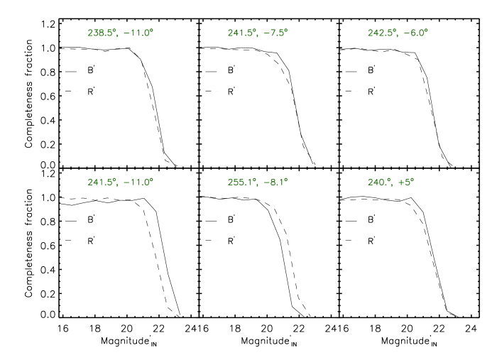
Figure 2.— Sample completeness diagrams for the CMa photometry from artificial star tests as a function of the input artificial star magnitude. Coupled with Fig. 3, this is a diagnostic of the photometric quality. We have restricted the tests to six fields that provide a good coverage of the range of latitudes and longitudes of the CMa over-density. As these tests were performed using instrumental magnitudes, we applied an approximate zero-point correction to each bandpass to shift the magnitudes to the flux calibrated system. Also, as we use de-reddened CMDs in this paper, we applied an appropriate shift to the input magnitude scale of each completeness curve, denoted by Magnitude${}^{\prime}_{\rm IN}$. We refer to the magnitude shifted B- and R-band completeness curves by B^′ and R^′ respectively in the panels. See Sec. 2 for further details.

These figures are given separately as a JPG file.

Figure 3.— Photometry diagnostic, based on artificial star tests. In each of the two groups of panels we provide magnitude scatter plots (upper) [recovered minus input magnitudes] as a function of the input magnitude, as well as the magnitude dependence of the error curve enclosing $\pm$34% of the stars (lower panels). They indicate that 68% of injected stars at B^′$\sim$22.6 mag and R^′$\sim$22 mag in these fields have a photometry error typically below 0.05 mag, and smaller still at brighter magnitudes. For the sake of clarity, we restricted this diagnostic check to a sub-set of six fields spanning the survey area, with some at similar positions to check the local and global photometric quality. For the meaning of B${}^{\prime}_{\rm IN}$ and R${}^{\prime}_{\rm IN}$, please see the meaning of Magnitude${}^{\prime}_{\rm IN}$ in Fig. 2.

This figure is given separately as a JPG file.

Figure 4.— CMD of an example ‘control field’ at (l,b)=(239.9^∘,-20^∘) from our survey (top) and its interpretation in terms of a synthetic MW model (bottom), which accounts only for the smooth and symmetric components (thin, thick disk, and halo). It shows that such fields comprise stars over a range of distances without prominent sub-structure along the line-of-sight. There is an absence of stars at B₀ $\lesssim$ 14.5 in the control field owing to detector saturation, and at B₀ $\gtrsim$ 22.5 because of the magnitude limit. It can be seen in the Galactic model CMD that fainter MS stars at a given colour are farther away. The marked density of model stars at [B₀ $>$ 22, (B-R)₀ $\sim$ 0.6-0.8 mag] in the synthetic CMD are ancient, metal-poor MS turn-off stars in the outer Galactic halo, but their number-density may be inaccurate.

Figure 5.— CMD of example control fields (right) at b =(+15^∘,+8^∘,+5^∘) from our survey (top-to-bottom), together with the CMDs for b =(-15^∘,-8^∘,-5^∘) (left). It illustrates that the structure of the CMDs for fields above and below the mid-plane differ over the full latitude range at l=240^∘.

This figure is given separately as a JPG file.

Figure 6.— We plot a sequence of CMDs across the Galactic plane along a fixed longitude (l$\sim$240^∘), running from b = +15^∘ to b = -20^∘. The text in each panel refers to the (l,b) position. The axes are labelled [B${}_{0}^{\prime}$, (B-R)${}_{0}^{\prime}$] because the photometry was de-reddened in two different steps (see Sec 2.2). Exceptions are the fields at b=+15^∘,+8^∘,+5^∘ and -20^∘, whose correct axis labelling is [B₀, (B-R)₀], but is excluded for the sake of clarity. The top-right panel shows photometry error bars (based on Fig. 3) at (B-R)${}_{0}^{\prime}$=0, which are typical for the bulk of these CMDs. We also show the de-reddening vector arising from the additional (i.e. post-SFD*) de-reddening step, which is described in Sec. 2.2. The 80% completeness limit (dashes), is included in two panels, illustrating the faint limiting magnitude of the photometry.

This figure is given separately as a JPG file.

Figure 7.— As Fig. 6, but for a sequence parallel to the Galactic plane at latitude (b$\sim$-8^∘), running from l $\sim$ 234 to l $\sim$ 258^∘. For other explanations, see Fig. 6.

This figure is given separately as a JPG file.

Figure 8.— Illustrating the extraction boxes used for the young and old MS star count estimates. The box to the right of the old MS is a reference box of MW stars. The 80% completeness limit is marked. See Sec. 5.1 for more on the extraction boxes.

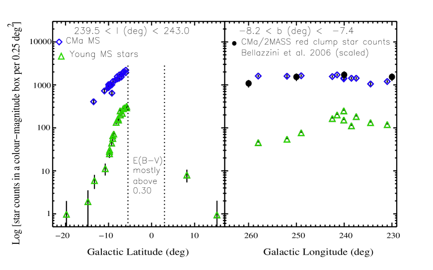
Figure 9.— Mapping the CMa stellar overdensity of young and old CMa MS stars as a function of Galactic latitude (left) and longitude (right). Only fields with median E(B-V)_SFD∗ below 0.30 mag are included. The open diamonds represent the density of old MS stars (as estimated in Sec. 5 and recorded in Table 1.); the triangles represent the young MS stars. In addition, CMa density estimates from red clump data (Bellazzini et al. 2006) are shown in the right panel, based on their Fig. 9, together with an assigned 20% error. The maximum of the Bellazzini et al. values has been scaled to match our results.

This figure is given separately as a JPG file.

Figure 10.— Surface density map of the area of sky sampled, including high extinction fields (median E(B-V)_SFD∗ $>$ 0.30 mag; diamonds). For the sake of clarity, the WFI field-of-view is over-sized. We note that the pointings at l$>$251^∘ were originally designed to be control fields. The (relative) number-density of old CMa MS stars (bottom) and young MS stars (top) is intensity-coded. One sees an over-density of old MS stars that is most likely centred below the Galactic mid-plane (also see Fig. 8), and exhibits a pronounced elongation in Galactic longitude. The young MS population is probably also centred below the mid-plane, but is substantially more localized in the longitude direction.

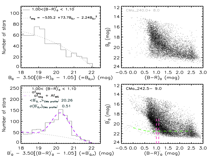
Figure 11.— Estimating the line-of-sight depth of CMa: We show the star-count distribution (left panels) and the associated CMD (right panels), for a reference star-field (top) and a field, (l,b) = (242.5^∘, -9.^∘) (bottom), near the presumed centre of the CMa over-density. The ‘thickness’ of the old MS, reflecting the l.o.s. extent is estimated in the colour interval bounded by vertical lines (dashes) in the bottom-right panel. As a guide to the photometric quality, the 80% completeness limit is also marked (horizontal and tilted dashes). In the bottom-left panel, the functional form from the top-left panel (short-dashes), together with a Gaussian function is fitted (long-dashes) to the histogram. The data in this panel are representative, and correspond to only one iteration of data re-sampling. See Sec. 5.1 for further explanations of the depth estimation.

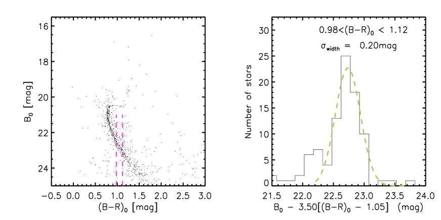
Figure 12.— Estimating the MS width of a reference stellar population, the globular cluster Pal 12. We have applied a similar procedure to that shown in Fig. 11. We extracted photometry from a narrow colour interval in the CMD (left-panel). We then fitted a Gaussian distribution (dashes, right-panel). The 1 $\sigma$ width data given in the right-panel is from one iteration of data re-sampling. For more information, see Sec. 6.2.

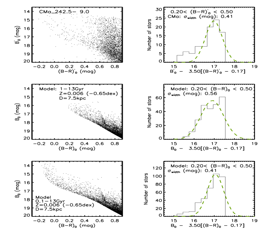
Figure 13.— Demonstrating the depth estimation method for the young MS population: We use same CMD (l,b = 242.5^∘, -9^∘) used to estimate the depth of the old CMa MS population (see Sec. 6.1). We show the young empirical MS (top-left) and a corresponding histogram of star counts (top-right) from one iteration of data re-sampling, together with a fitted Gaussian distribution (dashes). The other panels are for the adopted synthetic stellar populations. Additional details on the depth estimation can be found in the panels and in Sec. 6.2.

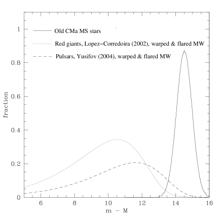
Figure 14.— Illustrating that none of the ‘smooth’ (locally axisymmetric) MW models for (l,b) = (241.5^∘,-7.5^∘) reach a maximum density near the distance modulus of the old CMa stars (solid). The area under each profile has been normalized to unity. The MW models are the warped, flared and inhomogeneity-free Galactic disk model from López-Corredoira et al. (2002) (short dashes) and the Yusifov (2004) model (long dashes). Model parameters are as given by those authors, except that we curtail the amplitude (z_w) of the warped López-Corredoira et al. disk from diverging to infinity by setting z_w(R$>$14 kpc) = z_w(R=14 kpc), where R is galacto-centric distance.

This figure is given separately as a JPG file.

Figure 15.— Illustrating that the CMa stellar over-density at (l,b) = (240^∘,-8^∘) (left) is absent in the control field at b=+8^∘ (middle), and is also absent in the (unreddened) Galaxy model CMD for b=-8^∘ (right). The Galactic model has been constructed by convolving a synthetic population (age =4-10 Gyr, -0.4 $>$[Z/Z_⊙]$>$ -0.5 dex), with the LC02 line-of-sight density profile of MW stars given in Fig. 14. Even though it has not been convolved with photometry errors, and contains no MW halo stars, a comparison of all three CMDs strongly disfavours the warped MW disk as a way to explain the old stellar over-density found in the CMa field. As we do not model the red plume of nearby ($\lesssim$ 1.5 kpc) late-type MS stars, the red boundary is set to (B-R)=2 mag.

Table 1Target information.

ID	l	b	E(B-V)${}_{\rm SFD*}^{\rm a}$ $\pm$ $\sigma$	$\Delta$ (B-R)0	NCMD	N${}_{\rm Old\,\,MS}$ $\pm$ $\sigma$	N${}_{\rm Young\,\,MS}$ $\pm$$\sigma$
	(deg)	(deg)	(mag)	(mag)
(1)	(2)	(3)	(4)	(5)	(6)	(7)	(8)
CMa_231.0- 8.0	230.989	-7.995	0.235 $\pm$ 0.016	-0.05	11964	1236 $\pm$ 85	117 $\pm$ 10
CMa_233.0-15.0	232.976	-14.997	0.063 $\pm$ 0.004	$\cdots$	5684	-51 $\pm$ 70	4 $\pm$ 2
CMa_233.0-14.0	232.985	-13.995	0.092 $\pm$ 0.009	0.00	7256	183 $\pm$ 50	7 $\pm$ 2
CMa_234.5- 8.0	234.482	-8.001	0.220 $\pm$ 0.009	-0.10	14641	1038 $\pm$ 77	133 $\pm$ 10
CMa_235.0-10.0	234.984	-9.996	0.188 $\pm$ 0.016	-0.03	10412	699 $\pm$ 80	36 $\pm$ 6
CMa_235.5-11.5	235.484	-11.504	0.135 $\pm$ 0.011	-0.06	9221	585 $\pm$ 66	12 $\pm$ 3
CMa_235.5- 5.0	235.528	-5.015	0.412 $\pm$ 0.034	$\cdots$	13195	$\cdots$	$\cdots$
CMa_236.5- 3.5	236.465	-3.505	0.740 $\pm$ 0.081	$\cdots$	11933	$\cdots$	$\cdots$
CMa_237.0-12.5	236.983	-12.494	0.118 $\pm$ 0.004	-0.10	8193	487 $\pm$ 67	13 $\pm$ 3
CMa_237.5- 9.0	237.478	-8.993	0.219 $\pm$ 0.032	-0.07	12360	1138 $\pm$ 75	86 $\pm$ 8
CMa_237.5- 8.0	237.480	-7.995	0.219 $\pm$ 0.018	-0.02	15668	1421 $\pm$ 96	182 $\pm$ 15
CMa_237.5- 6.0	237.483	-5.997	0.305 $\pm$ 0.022	$\cdots$	19815	$\cdots$	$\cdots$
CMa_237.5- 7.0	237.486	-7.020	0.287 $\pm$ 0.023	-0.00	16331	1804 $\pm$ 105	185 $\pm$ 14
CMa_238.5- 5.0	238.476	-4.993	0.489 $\pm$ 0.050	$\cdots$	15497	$\cdots$	$\cdots$
CMa_238.5-11.0	238.478	-10.976	0.141 $\pm$ 0.007	-0.09	10235	813 $\pm$ 65	12 $\pm$ 3
CMa_238.5- 6.5	238.481	-6.500	0.277 $\pm$ 0.030	-0.08	13545	1507 $\pm$ 100	186 $\pm$ 13
CMa_238.5- 7.5	238.484	-7.468	0.298 $\pm$ 0.021	-0.08	15544	1456 $\pm$ 114	111 $\pm$ 11
CMa_239.7- 9.2	239.680	-9.244	0.143 $\pm$ 0.004	-0.00	12876	993 $\pm$ 88	66 $\pm$ 7
CMa_239.7-10.0	239.681	-10.001	0.127 $\pm$ 0.007	0.00	12436	867 $\pm$ 74	27 $\pm$ 4
CMa_239.7- 6.0	239.687	-5.994	0.304 $\pm$ 0.021	$\cdots$	15882	$\cdots$	$\cdots$
CMa_239.7- 6.8	239.691	-6.754	0.338 $\pm$ 0.024	$\cdots$	15001	$\cdots$	$\cdots$
CMa_240.0+ 5.0	239.981	4.991	0.152 $\pm$ 0.004	$\cdots$	14213	-25 $\pm$ 121	8 $\pm$ 2
CMa_240.0-15.0	239.981	-15.000	0.100 $\pm$ 0.004	$\cdots$	5765	-129 $\pm$ 77	2 $\pm$ 1
CMa_240.0-20.0	239.985	-19.997	0.047 $\pm$ 0.002	$\cdots$	3169	2 $\pm$ 51	1 $\pm$ 1
CMa_240.0+15.0	239.986	14.996	0.052 $\pm$ 0.003	$\cdots$	3933	-39 $\pm$ 39	1 $\pm$ 1
CMa_240.0+ 8.0	239.988	8.000	0.109 $\pm$ 0.004	$\cdots$	9543	-25 $\pm$ 78	8 $\pm$ 2
CMa_240.0- 2.7	239.999	-2.693	0.531 $\pm$ 0.004	$\cdots$	1781	$\cdots$	$\cdots$
CMa_240.1- 7.9	240.078	-7.894	0.211 $\pm$ 0.020	0.14	13132	1374 $\pm$ 106	150 $\pm$ 11
CMa_240.1- 7.5	240.082	-7.503	0.228 $\pm$ 0.026	-0.21	13557	1467 $\pm$ 128	251 $\pm$ 16
CMa_240.1-13.5	240.083	-13.491	0.134 $\pm$ 0.009	-0.16	5795	407 $\pm$ 55	5 $\pm$ 2
CMa_240.5-10.0	240.482	-9.995	0.123 $\pm$ 0.004	0.12	11144	1007 $\pm$ 55	23 $\pm$ 4
CMa_240.5- 6.0	240.485	-5.996	0.239 $\pm$ 0.014	0.08	21239	2193 $\pm$ 115	318 $\pm$ 15
CMa_240.5- 6.8	240.490	-6.761	0.228 $\pm$ 0.015	0.06	19616	1783 $\pm$ 124	280 $\pm$ 15
CMa_240.5- 9.2	240.514	-9.225	0.125 $\pm$ 0.004	-0.09	9495	642 $\pm$ 64	59 $\pm$ 7
CMa_241.5- 7.5	241.480	-7.468	0.184 $\pm$ 0.013	0.10	18257	1698 $\pm$ 95	201 $\pm$ 15
CMa_241.5-11.0	241.482	-10.975	0.118 $\pm$ 0.006	0.02	11286	741 $\pm$ 87	10 $\pm$ 3
CMa_241.5- 9.5	241.482	-9.495	0.133 $\pm$ 0.004	0.03	14146	1018 $\pm$ 85	44 $\pm$ 6
CMa_241.5- 8.4	241.487	-8.442	0.151 $\pm$ 0.005	0.05	15248	1285 $\pm$ 87	131 $\pm$ 10
CMa_241.5- 6.5	241.487	-6.499	0.251 $\pm$ 0.019	0.11	19328	2028 $\pm$ 106	289 $\pm$ 15
CMa_241.5- 5.0	241.488	-4.978	0.343 $\pm$ 0.042	$\cdots$	22302	$\cdots$	$\cdots$
CMa_242.5- 8.0	242.482	-7.990	0.160 $\pm$ 0.009	0.07	17637	1543 $\pm$ 92	165 $\pm$ 12
CMa_242.5- 7.0	242.483	-7.016	0.193 $\pm$ 0.015	0.02	18419	1583 $\pm$ 139	216 $\pm$ 12
CMa_242.5- 9.9	242.484	-9.949	0.136 $\pm$ 0.017	-0.04	12451	929 $\pm$ 74	31 $\pm$ 5
CMa_242.5- 9.0	242.484	-8.994	0.129 $\pm$ 0.009	0.00	15397	1188 $\pm$ 80	72 $\pm$ 7
CMa_242.5- 6.0	242.486	-5.993	0.258 $\pm$ 0.019	0.02	19347	1943 $\pm$ 125	296 $\pm$ 19
CMa_243.0- 3.6	242.999	-3.630	0.508 $\pm$ 0.021	$\cdots$	9434	$\cdots$	$\cdots$
CMa_248.0-14.0	247.982	-13.993	0.164 $\pm$ 0.008	-0.08	6477	333 $\pm$ 61	5 $\pm$ 2
CMa_248.0-15.0	247.990	-14.999	0.168 $\pm$ 0.016	$\cdots$	5666	50 $\pm$ 69	4 $\pm$ 1
CMa_249.0-14.0	248.986	-13.997	0.146 $\pm$ 0.011	-0.07	7194	377 $\pm$ 49	8 $\pm$ 3
CMa_249.0- 8.0	248.996	-7.999	0.286 $\pm$ 0.016	-0.07	15215	1642 $\pm$ 99	77 $\pm$ 8
CMa_251.9- 2.8	251.904	-2.837	1.063 $\pm$ 0.066	$\cdots$	3493	$\cdots$	$\cdots$
CMa_252.0- 8.0	251.965	-8.004	0.296 $\pm$ 0.025	-0.05	15333	1608 $\pm$ 95	54 $\pm$ 7
CMa_252.0-15.0	251.977	-15.004	0.119 $\pm$ 0.004	$\cdots$	5118	-9 $\pm$ 67	2 $\pm$ 1

Table 2Target information. Continued

ID	l	b	E(B-V)${}_{\rm SFD*}^{\rm a}$ $\pm$ $\sigma$	$\Delta$ (B-R)0	NCMD	N${}_{\rm Old\,\,MS}$ $\pm$ $\sigma$	N${}_{\rm Young\,\,MS}$ $\pm$$\sigma$
	(deg)	(deg)	(mag)	(mag)
(1)	(2)	(3)	(4)	(5)	(6)	(7)	(8)
CMa_255.0- 3.0	254.974	-2.969	0.959 $\pm$ 0.064	$\cdots$	8660	$\cdots$	$\cdots$
CMa_255.0-15.0	254.986	-15.006	0.118 $\pm$ 0.005	$\cdots$	5164	-7 $\pm$ 65	1 $\pm$ 1
CMa_255.0- 8.0	254.988	-8.001	0.307 $\pm$ 0.041	$\cdots$	15506	$\cdots$	$\cdots$
CMa_257.9- 3.1	257.886	-3.099	1.566 $\pm$ 0.056	$\cdots$	2212	$\cdots$	$\cdots$
CMa_258.0-15.0	257.979	-15.001	0.152 $\pm$ 0.011	$\cdots$	5884	-141 $\pm$ 104	6 $\pm$ 2
CMa_258.0- 8.0	257.985	-7.979	0.260 $\pm$ 0.029	-0.08	18441	1677 $\pm$ 146	45 $\pm$ 6

References

- (1) Bellazzini, M., Ibata, R., Martin, N., Lewis, G. F., Conn, B., 2006, MNRAS, 366, 865 (B06)
- (2) Bellazzini, M., Ibata, R., Monaco, L., Martin, N., Irwin, M. J., et al., 2005, MNRAS, 354, 1263 (B05)
- (3) Belokurov, V., Zucker, D. B., Evans, N. W., Gilmore, G., Vidrih, S., et al. et al., 2006, ApJ, 637, 29
- (4) Bonifacio, P., Monai, S., & Beers, T. C., 2000, AJ, 120, 2065
- (5) Butler, D. J., Martínez-Delgado, D., 2005, AJ, 129, 2217
- (6) Bragaglia A., Tosi, M., Gloria A., Marconi G., 2006, MNRAS, 368, 1971
- (7) Cardelli, Jason A., Clayton, Geoffrey C., Mathis, John S., 2005, ApJ, 329, 33
- (8) Carraro, G., Vázquez, R A., Moitinho, A., Baume, G., 2005, ApJ, 630, 153
- (9) Conn, B., Martin, N. F., Lewis, G. F., Ibata, R. A., Bellazzini, M., et al., 2006, MNRAS, 367, 69
- (10) Cseresnjes, P., Alard, C., Guibert, J., 2000, A&A, 357, 871
- (11) Dinescu, D., Martínez-Delgado D., Girard, T., Peñarrubia J., Rix, H-W., et al., 2005, ApJ, 631, 49
- (12) Dolphin, A., Saha, A., Skillman, E. D., et al., AJ, 126, 187
- (13) Galadi-Enriquez, D., Trullols, E., Jordi, C., 2000, A&AS, 146, 169
- (14) Harris, W. E., 1996, AJ, 112, 1487
- (15) Harris, J., Zaritsky, D., 2004, AJ, 127, 1531
- (16) Ibata, R., Lewis, G., 1998, ApJ, 500, 575
- (17) Ibata, R., Irwin, M. J., Lewis, G. F., Ferguson, A. M. N., Tanvir, N., 2003, MNRAS, 340, 21
- (18) Johnston, K., Majewski, S. R., Siegel, H. M., Reid, I. N., & Kunkel, W. E., 1999, AJ, 118, 1719
- (19) Lance, C., 1988, ApJ, 334, 927
- (20) Landolt, A.U., 1992, AJ, 104, 340
- (21) López-Corredoira M., 2006, MNRAS, 369, 1911
- (22) López-Corredoira, M., Cabrera-Lavers A., Garzón, F., Hammersley, P. L., 2002, å, 394, 883
- (23) Martínez-Delgado D., Butler D., Rix H-W., Franco Y. I., Peñarrubia J., et al., 2005, ApJ, 633, 205
- (24) Martínez-Delgado D, Peñarrubia J., Butler D., Dinescu D.I., Rix H-W., 2005, Proc. IAU Colloquium 198, 1, 97-100, Eds Jerjen, H., Binggeli, B., Camb. Univ. Press (2005b)
- (25) Martínez-Delgado, D., Gómez-Flechoso, M. Á, Aparicio, A., Carrera, R., 2004, ApJ, 601, 242
- (26) Martínez-Delgado, D., Zinn, R., Carrera, R., Gallart, C., 2002, ApJ, 573, 19
- (27) Martínez-Delgado, D., Gallart, C., Aparicio, A., 1999, AJ, 118, 862
- (28) Martin N. F., Ibata, R. A., Bellazzini, M., Irwin, M. J., Lewis, G. F., et al., 2004, MNRAS, 348, 12 (2004a)
- (29) Martin N. F., Ibata, R. A., Lewis, G. F., Bellazzini, M., Irwin, M., et al., 2004, MNRAS, 355, L33 (2004b)
- (30) Martin, N. F., Ibata, R. A., Conn, B. C., Lewis, G. F., Bellazzini, M., et al., 2005, MNRAS, 362, 906
- (31) Martin, N. F., Irwin, M. J., Ibata, R. A., Conn, B. C., Lewis, G. F., et al., 2006, MNRAS, 367, 69
- (32) Newberg, H. J., Yanny, B., Rockosi, C., Grebel, E. K., Rix, H-W., et al., 2002, ApJ, 569, 245
- (33) Newberg, H. J., Yanny, B., Grebel, E. K., Hennessy, G., Ivezić Z., et al., 2003, ApJ, 596, 191
- (34) Moitinho, A., Vázquez, R. A.,; Carraro, G., Baume, G., Giorgi, E. E., et al., 2006, MNRAS, 368, 77
- (35) McConnachie, A., Peñarrubia J. & Navarro, J., astro-ph/0608687
- (36) Momany, et al., 2004, A&A, 421, 69
- (37) Momany, Y., Zaggia, S., Gilmore, G., Piotto, G., Carraro, G., et al., 2006, A&A, 451, 515,
- (38) Peñarrubia J., et al. 2005, ApJ, 626, 128
- (39) Peñarrubia J., Benson A., Martinez-Delgado D., & Rix H-W., ApJ, 645, 240
- (40) Piatek, S. & Pryor, C., 1995, AJ, 109, 1071
- (41) Schirmer, M., Erben, T., Schneider, P., Pietrzynski, G., Gieren, W., et al., 2003, A&A, 407, 869
- (42) Stetson, P. B., Hesser, J., Smecker-Hane T. A., 1998, PASP, 110, 533
- (43) Rodgers, A. W., Harding, P., & Sadler, E., 1981, ApJ, 244, 912
- (44) Robin, A., Reylé, C., Derri re, S., Picaud, S, 2003, A&A, 509, 523
- (45) Rocha-Pinto, H. J., Majewski, S. R., Skrutskie, Patterson, R. J., Nakanish, H., et al., 2006, ApJ, 640, 147
- (46) Vivas, A. K., Zinn, R., 2006, AJ, 132, 714
- (47) Yanny, B., et al., 2003, ApJ, 588, 824
- (48) Yusifov I., 2003, in The Magnetized Instellar Medium, Eds Uyanzker, B., Reich, W., & Wielebinski, R., Copernicus GmbH, Katlenburg-Lindau., 165