Spectropolarimetric survey of hydrogen-rich white dwarf stars

Abstract

We have conducted a survey of 61 southern white dwarfs searching for magnetic fields using Zeeman spectropolarimetry. Our objective is to obtain a magnetic field distribution for these objects and, in particular, to find white dwarfs with weak fields. We found one possible candidate (WD 0310$-$688) that may have a weak magnetic field of $-6.1\pm 2.2$ kG. Next, we determine the fraction and distribution of magnetic white dwarfs in the Solar neighborhood, and investigate the probability of finding more of these objects based on the current incidence of magnetism in white dwarfs within 20 pc of the Sun. We have also analyzed the spectra of the white dwarfs to obtain effective temperatures and surface gravities.

1. Introduction

White dwarfs are fossil remains of stellar evolution, and a study of the distribution of magnetic fields among white dwarfs may help elucidate the role played by magnetic fields in the evolution of low to intermediate mass stars.

Our current knowledge of the field distribution, i.e., the fraction of magnetic white dwarfs as a function of field strength (polar, surface average, or longitudinal field strength), is dictated by a compilation of surveys of various aims and field sensitivities. Spectroscopic surveys are useful in probing the Zeeman effect in the Balmer lines of hydrogen-rich DA white dwarfs, and may achieve field sensitivity of $\gtrsim 1$MG causing Zeeman splitting of $\Delta\lambda\gtrsim 20$Å in low-dispersion spectra (Vennes, 1999; Ferrario et al., 1998), or $\gtrsim 10$kG corresponding to $\Delta\lambda\gtrsim 0.2$Å in high-dispersion spectra of bright candidates (e.g., Koester et al., 1998). On the other hand, low-dispersion spectropolarimetric surveys of DA white dwarfs may achieve sensitivities of $\gtrsim 10$kG while offering increased accessibility to fainter white dwarfs (Schmidt & Smith, 1995).

Similar studies (e.g., Putney, 1997; Jordan et al., 1998; Schmidt et al., 2001) of the incidence of magnetic fields in non-DA white dwarfs (helium-line DB, or continuum-like DC) are more difficult because of the weakness of helium lines relative to hydrogen lines in stars with similar ages, although the presence of Zeeman-split metal lines may betray the presence of a magnetic field in such objects (e.g., Reid et al., 2001). Dichroism of continuous opacities induces optical circular polarization of the order of $V/I\approx 0.1B$%, where $B$ is expressed in MG (Kemp, 1970; Angel et al., 1981). Therefore, polarimetry of DC white dwarfs may achieve field sensitivity $\gtrsim 1$MG in high-quality surveys ($V/I\gtrsim 0.1$%) or more generally $\gtrsim 10$MG ($V/I\gtrsim 1$%).

Spectroscopic and polarimetric surveys have accumulated sufficient data to describe the field distribution $\gtrsim 1$MG in all nearby white dwarfs (DA and non-DA), while only a fraction of the data is available to describe the distribution $\gtrsim 0.1$MG among brighter hydrogen-rich DA white dwarfs. The aim of spectropolarimetric surveys is to complement spectroscopic surveys and provide data for fainter DA candidates with even lower fields in the 10kG-1MG range. Kawka et al. (2003) derived the field distribution in the local white dwarf census of Holberg et al. (2002). The incidence of magnetic field appears constant per decade of field strength from 0.1MG to close to 1000 MG. Since the estimate of Kawka et al. (2003), which included the low-field magnetic white dwarf 40 Eri B (Fabrika et al., 2000), Aznar Cuadrado et al. (2004) added the low-field white dwarf LTT 9857 (3.1 kG) to the local census (i.e., within 20 pc of the Sun) thereby extending the field distribution well below 10 kG. The origin of fields in white dwarf stars is more difficult to establish quantitatively. Kawka (2004) and Kawka & Vennes (2004) revisited some assumptions about the magnetic white dwarf space density and the corresponding space density of their likely Ap/Bp progenitors. They concluded that our current knowledge of stellar formation rate and evolutionary time scales cannot account for the present day density of magnetic white dwarfs. Low field white dwarfs are also not accounted for, which prompted Kawka & Vennes (2004) to suggest that additional progenitors are required.

In §2 we present spectropolarimetry of 61 white dwarfs with $V\lesssim 16.4$ and $\delta<-30^{\circ}$, among which 55 have $V\lesssim 15.0$ and 5 are in close binaries. We also present spectropolarimetry of 4 subdwarf B (sdB) stars, where two of these were misclassified as white dwarfs. This complements a spectropolarimetric survey for magnetic fields among northern hemisphere white dwarfs carried out by Schmidt & Smith (1995). That survey sampled some 169 DA white dwarfs and resulted in the discovery of four new magnetic white dwarfs with fields between $\sim$$10^{5}$ and $10^{9}$ G. We present our analyses of our observations in §3 and in §4 we discuss the properties of the local population of magnetic white dwarfs. Finally, in §5 we summarize our results. Appendix A tabulates the properties of all magnetic white dwarfs known to date.

2. Observations

2.1. Spectropolarimetry

The data for the survey of magnetic fields in southern white dwarfs were acquired using the 74-inch telescope at the Mt. Stromlo Observatory with the Steward Observatory CCD Spectropolarimeter. The original instrument is described in Schmidt et al. (1992). The instrument setup was updated and modified for the 74-inch telescope, with an improved camera lens and a thinned, back illuminated LORAL $1200\times 800$ CCD with near unity quantum efficiency and $<6$e^- read noise. The $f/18$ Cassegrain telescope beam was adapted to the $f/9$ spectrograph optics with a small converging lens placed in front of the slit. A 964 lines mm^-1 grating blazed at 4639 Å was used which gave a dispersion of 2.62 Å per pixel. Circularly polarized spectra of white dwarfs were obtained over a region which includes H$\alpha$, H$\beta$ and H$\gamma$, with a spectral resolution of $\sim 9$ Å. The data were acquired in multiple waveplate sequences. The length of an exposure, which varied from 360 to 2400 seconds depending on the brightness of the object and the seeing conditions, is the time required for one waveplate sequence to be completed. One waveplate sequence is a series of four exposures at different quarter-waveplate orientations that produces two complementary images in opposite senses of circular polarization. These are used to obtain the degree of circular polarization as a function of wavelength $v_{\lambda}$, as well as the total (unpolarized) spectral flux $F_{\lambda}$. The slit width was generally set at $2.4^{\prime\prime}$, however it was increased to $3.6^{\prime\prime}$ when the seeing deteriorated. The observations were conducted on 2000 October 27-29, November 3, 5, 25-26, December 1-4, 23-28, 31, 2001 January 1, 18-20, 27, and February 17, 18, 21, 22 and 25.

2.2. Complementary Spectroscopy

Additional spectroscopy of many of the white dwarfs in the survey have been obtained using the 74-inch telescope with the Cassegrain spectrograph equipped with a 300 line mm^-1 grating blazed at 5000 Å and a 2k $\times$ 4k CCD binned 2 $\times$ 2. This resulted in a wavelength dispersion of 2.85 Å per pixel and a spectral range of about 3500 Å to 6400 Å providing a spectral resolution of $\sim 8$ Å. The observations were carried out on 1998 May 26, June 18, 2001 February 28, March 2, 4, 5, 7, 8, September 13, 15, 16 and October 25 - 28, and 2002 January 7, 8, March 8 and April 3. The purpose of obtaining these additional spectra was to have spectral coverage of the upper Balmer line series, not covered by the spectropolarimeter, and to constrain the temperature and gravity of the white dwarfs. For many of the hot white dwarfs in our sample, we have re-analyzed the spectra from Vennes et al. (1996), Vennes et al. (1997), Ferrario et al. (1997a), Vennes (1999) and Kawka et al. (2004).

3. Analysis

The mean longitudinal magnetic field for a specific absorption line is measured at each wavelength using the weak-field approximation (Angel et al., 1973)

$$B_{\ell}=\frac{vF}{4.67\times 10^{-13}\lambda^{2}\frac{dF}{d\lambda}}$$ (1)

where $\lambda$ is the wavelength in Å, $B_{\ell}$ is the longitudinal magnetic field strength in G, $F$ is the total spectral flux (i.e., the total intensity, $I$) and $v=V/I$ is the degree of circular polarization. The flux gradient $dF/d\lambda$ is calculated from a pseudo-Lorentzian fit to the line profile of the normalized flux. The fitted line profile is used in this procedure instead of the observed profile to reduce the effects of statistical noise in the flux distribution and is appropriate when the Zeeman splitting is not resolved. For a typical white dwarf this is a reasonable approximation for $B\lesssim 1$ MG. The quoted $B_{\ell}$ for a given star and epoch is computed from the weighted average of measurements at various wavelength bins across a profile, followed by a weighted average for the lines observed, here H$\alpha$, H$\beta$, and H$\gamma$.

The uncertainty in $B_{\ell}$ at each wavelength bin includes two sources of noise. The first and most important contribution is derived from the statistical fluctuation in the circular polarization spectrum. This is measured in the far wings of the absorption line and converted to an uncertainty in $B_{\ell}$ (which we call $\sigma_{i}$) using standard error propagation techniques. Assuming all errors are statistical, these point-by-point uncertainties combine to an uncertainty in the value of $B_{\ell}$ for the entire line as $\sigma_{noise}=1/\sqrt{(}\sum 1/\sigma_{i}^{2})$.

The second contribution to the uncertainty of a derived field strength stems from the uncertainty in fitting the pseudo-Lorentzian line profile (i.e., they are estimated from the root-mean-square deviation of the data from the best-fit line profile), and is included as an independent noise source $\sigma_{prof}$. The total uncertainty in $B_{\ell}$ for a given absorption line is then taken to be $\sigma_{B_{\ell}}=\sqrt{\sigma^{2}_{prof}+\sigma^{2}_{noise}}$.

Table 1Survey of white dwarfs.

WD	UT Date	$B_{\ell}$ (kG)	WD	UT Date	$B_{\ell}$ (kG)
0018$-$339	25/11/2000	$0.23\pm 13.52$	0859$-$039	23/12/2000	$-9.41\pm 8.61$
	02/12/2000	$22.86\pm 16.66$		26/12/2000	$5.97\pm 8.00$
	04/12/2000	$-5.21\pm 12.36$	0950$-$572	04/12/2000	$1.25\pm 8.55$
0047$-$524	01/12/2000	$-10.51\pm 13.16$		24/12/2000	$1.03\pm 10.36$
0050$-$332	25/12/2000	$-0.28\pm 9.48$	0954$-$710	02/12/2000	$0.01\pm 4.32$
0106$-$358	01/12/2000	$2.97\pm 17.85$	0957$-$666	01/12/2000	$-9.73\pm 14.42$
	24/12/2000	$-2.15\pm 11.85$	0958$-$073	27/12/2000	$0.01\pm 4.32$
0107$-$342	01/12/2000	$-17.57\pm 12.28$	1013$-$050	25/02/2001	$-18.31\pm 32.80$
	24/12/2000	$-5.17\pm 5.70$	1022$-$301	21/02/2001	$-4.53\pm 27.04$
0126$-$532	05/11/2000	$12.65\pm 17.25$	1042$-$690	23/12/2000	$-20.45\pm 8.96$
	26/11/2000	$7.18\pm 8.08$	1053$-$550	19/01/2001	$-3.74\pm 7.53$
0131$-$164	26/12/2000	$23.27\pm 12.45$		20/01/2001	$-12.19\pm 9.18$
0141$-$675	27/10/2000	$2.93\pm 5.44$		27/01/2001	$1.55\pm 8.13$
	03/11/2000	$-1.68\pm 4.65$	1056$-$384	01/01/2001	$5.90\pm 5.06$
0255$-$705	28/10/2000	$0.27\pm 5.43$	1121$-$507	17/02/2001	$-0.47\pm 7.54$
0310$-$688	28/10/2000	$-6.09\pm 2.24$		18/02/2001	$-6.03\pm 7.98$
0325$-$857	23/12/2000	$7.16\pm 6.27$	1153$-$484	19/01/2001	$-10.41\pm 7.89$
0341$-$459	25/11/2000	$10.73\pm 8.37$		20/01/2001	$2.61\pm 3.86$
	26/11/2000	$4.20\pm 13.62$	1236$-$495	20/01/2001	$-2.58\pm 6.23$
0419$-$487	26/11/2000	$-0.23\pm 9.30$	1257$-$723	21/02/2001	$-7.79\pm 8.01$
	24/12/2000	$5.06\pm 41.61$	1323$-$514	17/02/2001	$-1.84\pm 8.18$
	26/12/2000	$6.08\pm 13.78$		18/02/2001	$-2.24\pm 8.88$
	18/01/2001	$-22.37\pm 27.30$	1407$-$475	17/02/2001	$13.34\pm 8.02$
0446$-$789	03/11/2000	$-7.73\pm 8.40$	1425$-$811	18/02/2001	$2.75\pm 5.13$
	24/12/2000	$-10.60\pm 5.76$	1529$-$772	25/02/2001	$87.05\pm 143.60$
0455$-$282	26/12/2000	$5.57\pm 15.84$	1544$-$377	18/02/2001	$-5.88\pm 7.68$
0501$-$289	26/12/2000	$-5.60\pm 10.35$		21/02/2001	$-0.25\pm 6.45$
0509$-$007	25/12/2000	$6.77\pm 9.78$	1616$-$591	21/02/2001	$7.27\pm 8.92$
0549$+$158	26/12/2000	$11.12\pm 9.18$		22/02/2001	$-8.66\pm 9.96$
0621$-$376	02/12/2000	$-11.12\pm 10.11$	1620$-$391	21/02/2001	$-2.96\pm 2.60$
0646$-$253	26/12/2000	$6.61\pm 6.63$	1628$-$873	22/02/2001	$7.45\pm 6.24$
0652$-$563	21/02/2001	$-4.56\pm 59.48$	1659$-$531	21/02/2001	$-1.06\pm 5.70$
0701$-$587	25/11/2000	$-0.21\pm 7.53$	1724$-$359	25/02/2001	$11.62\pm 25.06$
	24/12/2000	$-8.44\pm 10.16$	2007$-$303	27/10/2000	$5.50\pm 8.07$
0715$-$703	28/12/2000	$-2.16\pm 17.79$		29/10/2000	$3.68\pm 3.78$
	31/12/2000	$-43.64\pm 21.84$	2039$-$682	05/11/2000	$-6.00\pm 6.40$
	01/01/2001	$-7.06\pm 7.83$	2105$-$820	28/10/2000	$3.39\pm 4.98$
	17/02/2001	$-11.87\pm 10.95$	2115$-$560	05/11/2000	$-1.38\pm 7.05$
0718$-$316	02/12/2000	$51.21\pm 37.70$	2159$-$754	25/11/2000	$-7.75\pm 8.55$
0721$-$276	28/12/2000	$-10.09\pm 12.58$		02/12/2000	$-11.84\pm 7.18$
0732$-$427	27/12/2000	$0.71\pm 7.29$	2211$-$495	02/12/2000	$6.57\pm 5.32$
	21/02/2001	$6.46\pm 7.46$	2232$-$575	04/12/2000	$11.49\pm 10.17$
0740$-$570	27/12/2000	$-5.48\pm 13.54$	2329$-$291	24/12/2000	$0.19\pm 5.80$
0821$-$252	04/12/2000	$-576.34\pm 106.74$		25/12/2000	$7.07\pm 6.74$
	01/01/2001	$-698.81\pm 134.97$	2331$-$475	25/12/2000	$-2.18\pm 16.84$
	25/02/2001	$-538.19\pm 154.04$	2337$-$760	03/12/2000	$11.45\pm 19.98$
0839$-$327	25/11/2000	$2.89\pm 2.76$		04/12/2000	$11.19\pm 9.96$
0850$-$617	25/11/2000	$4.58\pm 12.58$	2359$-$434	27/10/2000	$3.41\pm 4.42$
	26/11/2000	$18.53\pm 12.96$

Figure 1.— Circular polarization spectra of the white dwarfs listed in Table 2. Each spectrum is separated by 0.10 for better visualization and the Balmer lines (H$\alpha$, H$\beta$ and H$\gamma$) are indicated by the dotted vertical lines.

Figure 2.— Circular polarization spectra of the EUV-selected white dwarfs (Table 2) and close binary stars (Table 3).

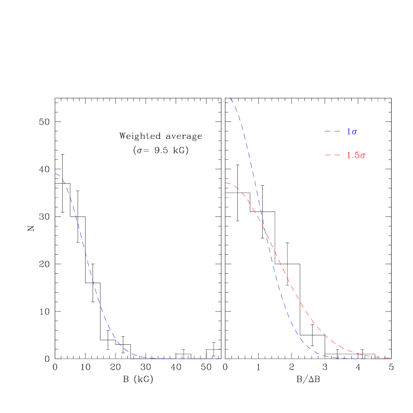
The results are tabulated in Table 1 and displayed as circular polarization spectra in Figures 1 and 2. The survey for magnetism yielded no detections of magnetism (those where the signal-to-noise ratio in the derived field strength clearly exceeds 3.0) with the possible exception of WD 0310$-$688. For an intrinsically nonmagnetic sample, one would expect that a histogram of the measured values of $B_{\ell}$ should approximate a Gaussian whose width is the mean uncertainty $\sigma_{B_{\ell}}$. However, as shown in Figure 3 the 9.5 kG width of the distribution is $\sim 50\%$ larger than the mean uncertainty. This could be due to the stars having weak magnetic fields of the order of a few kG, but we believe a more likely explanation is that our purely statistical estimates underrepresent the true uncertainties. For example, seeing and guiding variations, fluxing errors, and polarimetric calibration uncertainties can all affect the derived polarization spectra but have not been included in the analysis above. Similar conclusions were reached for the northern survey by Schmidt & Smith (1995). Therefore, in this paper all magnetic field measurements have been increased by 50% over their purely statistical values including the values in Table 1.

Figure 3.— Number distribution of measured magnetic field strengths ($N_{\rm total}=86$) compared to a gaussian distribution with $\sigma=9.5$ kG (left), and the number distribution of the measurements divided by their error and compared to a normalized gaussian distribution (right).

Table 2Survey of white dwarfs.

WD	Other Names	mV	$T_{eff}$	$\log{g}$	M	$d$
		(mag)	(K)	(cgs)	(M⊙)	(pc)
0018$-$339	GD 603, BPM 46232	14.62	$19460\pm 250$	$7.87\pm 0.05$	$0.55\pm 0.03$	63
0047$-$524	BPM 16274, L219-48	14.16	$17660\pm 180$	$7.82\pm 0.04$	$0.52\pm 0.02$	49
0050$-$332	GD 659, EUVE J0053-329	13.36	$35840\pm 250$	$7.90\pm 0.05$	$0.61\pm 0.02$	60
0106$-$358	GD 683, EUVE J0108-355	15.80	$29380\pm 400$	$7.86\pm 0.10$	$0.57\pm 0.05$	158
0126$-$532	BPM 16501, LTT 805	14.48	$16010\pm 160$	$7.94\pm 0.04$	$0.58\pm 0.02$	48
0131$-$164	GD 984, EUVE J0134-161	13.8	$45640\pm 1220$	$7.82\pm 0.07$	$0.59\pm 0.03$	91
0141$-$675	LTT 934, LHS 145	13.90	$6460\pm 160$	$8.04\pm 0.44$	$0.61\pm 0.24$	9
0255$-$705	LHS 1474, BPM 2819	14.08	$10620\pm 90$	$8.28\pm 0.06$	$0.78\pm 0.04$	21
0310$-$688	LB 3303, EG 21	11.40	$15480\pm 80$	$8.02\pm 0.02$	$0.62\pm 0.01$	11
0325$-$857	LB 9802	13.9	$15580\pm 200$	$8.36\pm 0.05$	$0.83\pm 0.03$	27
0341$-$459	BPM 31594, L300-34	15.03	$11700\pm 250$	$8.20\pm 0.10$	$0.73\pm 0.06$	40
0446$-$789	BPM 3523, L31-99	13.47	$22760\pm 390$	$7.70\pm 0.06$	$0.48\pm 0.03$	47
0455$-$282	MCT 0455-2812	13.95	$55680\pm 1410$	$7.90\pm 0.09$	$0.65\pm 0.04$	101
0509$-$007	EUVE J0512-006, RE J0512-004	13.83	$32400\pm 320$	$7.28\pm 0.09$	$0.36\pm 0.03$	107
0549$+$158	GD 71, LTT 11733	13.06	$33000\pm 190$	$7.84\pm 0.04$	$0.57\pm 0.02$	51
0621$-$376	EUVE J0623-376, RE J0623-374	12.09	$59800\pm 1810$	$7.23\pm 0.11$	$0.45\pm 0.02$	80
0646$-$253	EUVE J0648-253, RE J0648-252	13.65	$27720\pm 310$	$7.91\pm 0.04$	$0.59\pm 0.03$	53
0652$-$563	EUVE J0653$-$564	16.40	$33480\pm 620$	$8.92\pm 0.13$	$1.16\pm 0.06$	99
0701$-$587	BPM 18394, L184-75	14.46	$14800\pm 500$	$8.32\pm 0.08$	$0.81\pm 0.05$	35
0715$-$703	EUVE J0715-704, RE J0715-702	14.18	$42640\pm 710$	$7.81\pm 0.08$	$0.58\pm 0.03$	105
0721$-$276	EUVE J0723-277, RE J0723-274	14.52	$36500\pm 400$	$7.92\pm 0.08$	$0.62\pm 0.04$	102
0732$-$427	BPM 33039, LTT 2884	14.16	$14540\pm 370$	$8.15\pm 0.06$	$0.70\pm 0.04$	33
0740$-$570	BPM 18615, L185-53	15.06	$19760\pm 290$	$8.20\pm 0.06$	$0.74\pm 0.04$	62
0800$-$533	BPM 18764, L242-83	15.76	$20010\pm 500$	$7.86\pm 0.08$	$0.55\pm 0.04$	110
0821$-$252	EUVE J0823$-$254	16.40	$39800\pm 1400$	$9.23\pm 0.17$	$1.27\pm 0.06$	81
0839$-$327	LFT 600, LTT 3218	11.90	$9340\pm 60$	$8.11\pm 0.06$	$0.66\pm 0.04$	7
0848$-$730	BPM 5102, L63-60	15.30	$16800\pm 350$	$7.96\pm 0.08$	$0.59\pm 0.04$	72
0850$-$617	BPM 5109, L139-26	14.73	$19620\pm 340$	$8.04\pm 0.06$	$0.64\pm 0.03$	60
0859$-$039	EUVE J0902-041, RE J0902-040	13.19	$23560\pm 290$	$7.89\pm 0.04$	$0.57\pm 0.02$	38
0950$-$572	BPM 19738, L189-36	14.94	$13900\pm 600$	$7.84\pm 0.10$	$0.52\pm 0.05$	57
0954$-$710	BPM 6082, L64-27	13.48	$14280\pm 240$	$7.71\pm 0.06$	$0.46\pm 0.03$	32
1022$-$301	EUVE J1024$-$303, RE J1024$-$302	16.09	$34700\pm 700$	$9.05\pm 0.12$	$1.21\pm 0.05$	78
1053$-$550	LTT 4013, BPM 20383	14.32	$14000\pm 330$	$8.11\pm 0.10$	$0.67\pm 0.06$	36
1056$-$384	EUVE J1058-387, RE J1058-384	14.08	$27800\pm 420$	$8.02\pm 0.08$	$0.65\pm 0.04$	60
1121$-$507	BPM 20912, L251-24	14.86	$15620\pm 220$	$7.93\pm 0.06$	$0.57\pm 0.03$	57
1223$-$659	BPM 7543, L104-2	13.97	$7740\pm 70$	$8.13\pm 0.11$	$0.67\pm 0.07$	13
1236$-$495	LTT 4816, LFT 931	13.96	$11870\pm 130$	$8.84\pm 0.04$	$1.11\pm 0.02$	15
1257$-$723	BPM 7961, L69-47	15.18	$16380\pm 430$	$7.98\pm 0.10$	$0.60\pm 0.05$	66
1323$-$514	LFT 1004, LTT 5178	14.60	$18280\pm 220$	$7.92\pm 0.04$	$0.57\pm 0.02$	58
1407$-$475	BPM 38165, L332-123	14.31	$21080\pm 400$	$8.00\pm 0.06$	$0.63\pm 0.03$	54
1425$-$811	BPM 784, LTT 5712	13.75	$12600\pm 240$	$8.17\pm 0.06$	$0.71\pm 0.04$	24
1529$-$772	EUVE J1535$-$774	16.40	$49200\pm 1800$	$8.95\pm 0.16$	$1.18\pm 0.07$	119
1544$-$377	LTT 6302, L481-60	12.80	$10840\pm 80$	$8.27\pm 0.06$	$0.77\pm 0.04$	12
1616$-$591	BPM 24047, LTT 6501	15.08	$13950\pm 260$	$7.81\pm 0.07$	$0.51\pm 0.03$	62
1620$-$391	CD-38 10980, EUVE J1623-392	11.01	$23860\pm 390$	$8.02\pm 0.06$	$0.64\pm 0.03$	13
1628$-$873	BPM 890, L8-61	14.58	$11160\pm 190$	$8.29\pm 0.07$	$0.78\pm 0.04$	29
1659$-$531	BPM 24601, L268-92	13.47	$14660\pm 190$	$8.02\pm 0.04$	$0.62\pm 0.02$	27
1709$-$575	LTT 6859, BPM 24723	15.10	$16800\pm 320$	$7.87\pm 0.07$	$0.54\pm 0.03$	70
1724$-$359	EUVE J1727$-$360, RE J1727$-$355	15.46	$32000\pm 250$	$9.00\pm 0.06$	$1.20\pm 0.03$	58
1953$-$715	LTT 7875, BPM 12843	15.15	$18200\pm 480$	$7.97\pm 0.10$	$0.60\pm 0.05$	72
2007$-$303	LTT 7987, L565-18	12.18	$14840\pm 170$	$7.92\pm 0.04$	$0.57\pm 0.02$	16
2039$-$682	LTT 8190, BPM 13491	13.53	$16190\pm 220$	$8.47\pm 0.04$	$0.90\pm 0.03$	22
2105$-$820	BPM 1266, LTT 8381	13.62	$10660\pm 90$	$8.26\pm 0.06$	$0.76\pm 0.04$	18
2115$-$560	LTT 8452, BPM 27273	14.28	$9740\pm 80$	$8.30\pm 0.08$	$0.79\pm 0.05$	20
2159$-$754	LTT 8816, BPM 14525	15.06	$9040\pm 80$	$8.95\pm 0.12$	$1.17\pm 0.04$	14
2211$-$495	EUVE J2214-493, RE J2214-491	11.71	$63840\pm 1550$	$7.45\pm 0.10$	$0.51\pm 0.02$	57
2232$-$575	LTT 9082, BPM 27891	14.96	$15750\pm 290$	$7.75\pm 0.08$	$0.48\pm 0.04$	67
2331$-$475	EUVE J2334-472, RE J2334-471	13.42	$52060\pm 1670$	$7.92\pm 0.12$	$0.65\pm 0.05$	75
2336$-$079	GD 1212, GJ 4355	13.75	$11010\pm 210$	$8.05\pm 0.15$	$0.63\pm 0.09$	23
2337$-$760	LTT 9648, BPM 15727	14.66	$13800\pm 280$	$7.41\pm 0.08$	$0.32\pm 0.04$	63
2351$-$368	LHS 4041, LTT 9774	15.1	$14540\pm 320$	$8.00\pm 0.06$	$0.61\pm 0.03$	57
2359$-$434	LTT 9857, BPM 45338	13.05	$8570\pm 50$	$8.60\pm 0.06$	$0.98\pm 0.04$	7

Table 3Close binary stars.

WD	Other Names	mV	Spectral Type	$T_{eff}$	$\log{g}$	References
		(mag)		(K)	(cgs)
0419-487	LTT 1951, BPM 31852	14.36	DA+dMe	$7005\pm 140$	$7.72\pm 0.19$	1
0718-316	EUVE J0720-317, RE J0720-318	14.82	DAO+dMe	$52400\pm 1800$	$7.68\pm 0.10$	2
0957-666	BPM 6114, L101-26	14.60	DD	$27047\pm 398$	$7.28\pm 0.08$	1
1013-050	EUVE J1016-053	14.20	DAO+dMe	$54800\pm 1300$	$7.70\pm 0.10$	2
1042-690	BPM 6502, LTT 3943	13.09	DA+dMe	$19960\pm 400$	$7.86\pm 0.09$	3

References. — (1) Bragaglia et al. (1995); (2) Vennes et al. (1997); (3) This work

Balmer line spectra provide insights into the temperature and density structure of white dwarf atmospheres represented by the parameters $T_{\rm eff}$ and $\log{g}$. We computed a new grid of models supporting a ($T_{\rm eff}$, $\log{g}$) analysis: the grid of models extend from $T_{\rm eff}=4500$ to 6500 K (in steps of 500 K) at $\log{g}=7.0$, 8.0, and 9.0, from $T_{\rm eff}=7000$ to 16000 K (in steps of 1000 K), from 18000 to 32000 K (in steps of 2000 K), and from 36000 to 84000 K (in steps of 4000 K) at $\log{g}=7.0$ to 9.5 (in steps of 0.25 dex). Convective energy transport in cooler atmospheres is included by applying the Schwarzschild stability criterion and by using the mixing-length formalism described by Mihalas (1978), where we have assumed the ML2 parameterization of the convective flux (Fontaine et al., 1981) and adopting $\alpha=0.6$ (Bergeron et al., 1992b). The equation of convective energy transport was fully linearized within the Feautrier solution scheme and subjected to the constraint that $\mathcal{F}_{\rm total}=\sigma_{R}T^{4}_{\rm eff}=\mathcal{F}_{\rm conv}+\mathcal{F}_{\rm rad}$. The dissolution of the hydrogen energy levels in the high-density atmospheres of white dwarfs was calculated using the formalism of Hummer & Mihalas (1988) and following the treatment of Hubeny et al. (1994). See Kawka & Vennes (2006) for more detail of the procedure. The calculated level occupation probabilities are then explicitly included in the calculation of the line and continuum opacities. The Balmer line profiles are calculated using the tables of Stark-broadened H I line profiles of Lemke (1997) convolved with normalized resonance line profiles.

The observed Balmer lines (H$\alpha$/H$\beta$ to H$\epsilon$/H8) were fitted with model spectra using $\chi^{2}$ minimization techniques and the quoted uncertainties are statistical only ($1\sigma$) and do not take into account possible systematic effects in model calculations or data acquisition and reduction procedures. We used the mass-radius relations of Benvenuto & Althaus (1999) with a hydrogen envelope of $M_{H}/M_{*}=10^{-4}$ and a metallicity of Z=0 to convert the ($T_{\rm eff}$, $\log{g}$) measurements into white dwarf masses. For two white dwarfs (WD 0621-376 and WD 2211-495) we have used the mass-radius relations of Wood (1995) to determine their masses, since the mass-radius relations of Benvenuto & Althaus (1999) did not extend to the very high temperatures of these stars.

Table 4Stars from the survey that are not DA white dwarfs.

WD	Other Names	mV	Spectral Type	$T_{eff}$	$\log{g}$	$\log{(N_{He}/N_{H})}$	References
		(mag)		(K)	(cgs)
0107-342	GD 687, MCT 0107-3416	13.93	sdB	$24350\pm 100$	$5.32\pm 0.02$	-2.38	1
0501-289	MCT 0501-2858, EUVE J0503-288	13.9	DO	$68600\pm 1800$	$7.20\pm 0.07$	$\gtrsim 1.7$	2
0958-073	PG 0958-073, GD 108	13.56	sdB	$27760\pm 670$	$5.60\pm 0.11$	$\lesssim-3.0$	3
1153-484	BPM 36430, L 325-214	12.86	sdB	$30080\pm 660$	$5.15\pm 0.10$	$\lesssim-3.0$	3
2329-291	GD 1669	13.88	sdB	$34126\pm 100$	$5.77\pm 0.02$	-1.36	1

References. — (1) Lisker et al. (2005); (2) Vennes et al. (1998); (3) This work

The white dwarfs from the present study are presented in 3 different tables. Table 2 presents the DA white dwarfs that were assumed to follow single star evolution, white dwarfs in wide binaries are also included in this table. This table includes EUVE-selected ultramassive white dwarfs, which are indicated. White dwarfs in close binaries are presented in Table 3. And finally Table 3 presents the non-DA stars in our spectropolarimetric survey, which comprise of one DO white dwarf and 4 sdB stars.

3.1. Single white dwarfs

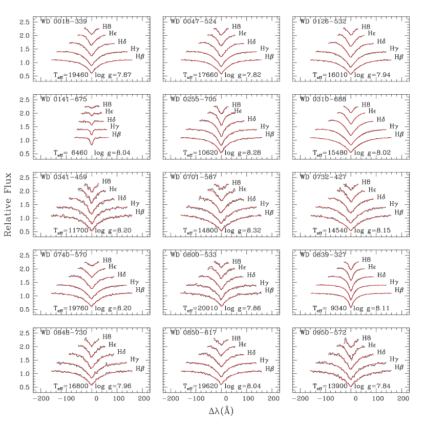
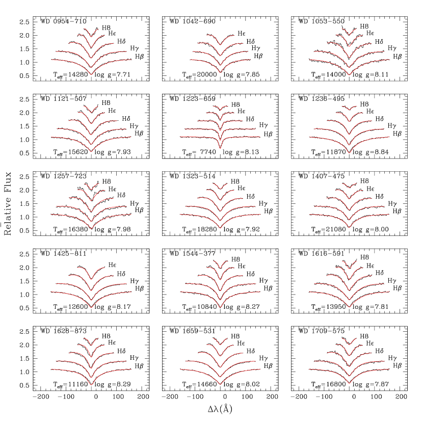
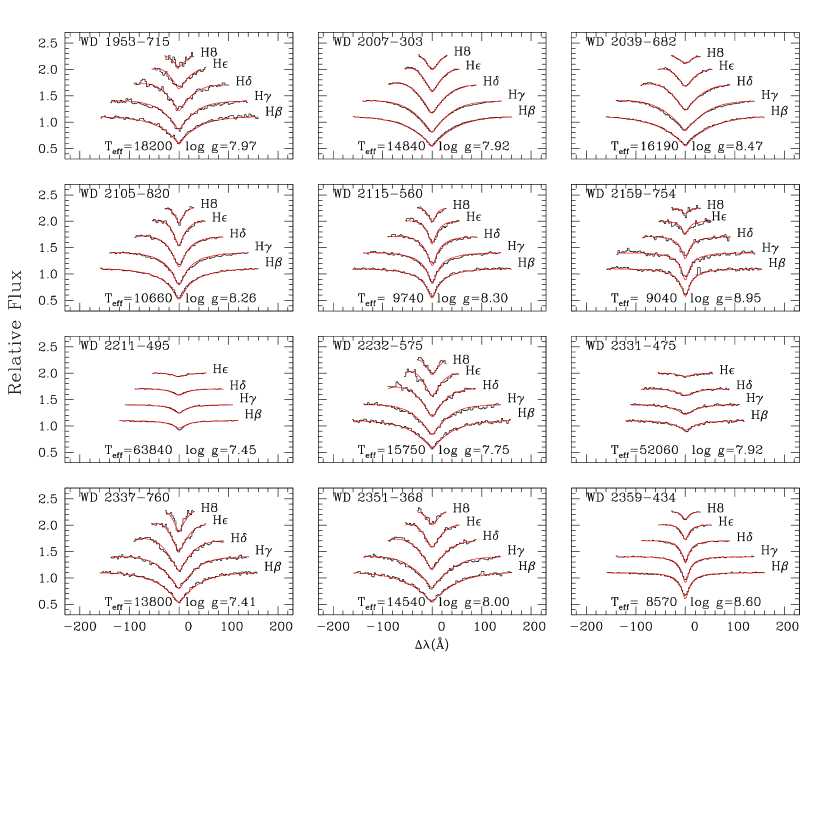
Table 2 presents the observed white dwarfs with their apparent magnitude, effective temperature, surface gravity and the distance. The distance was calculated from the apparent and absolute magnitudes. For 55 of these stars, spectropolarimetry was obtained. We have used the complementary spectra that cover the higher Balmer lines to determine their effective temperature and surface gravity by comparing these spectra to a grid of synthetic model spectra. Figure 4 shows the Balmer line profile fits to the observed spectra, which have not been previously published.

Figure 4.— Balmer line profile fits to the white dwarfs listed in Table 2.

Figure 4.— Continued

Figure 4.— Continued

Magnetic properties of several stars in this spectropolarimetric survey have been discussed in the literature, therefore these properties will be summarized and compared to the results of this study.

Figure 5.— The flux (top) and circular polarization (bottom) spectra of WD 0310$-$688. The polarization spectrum is compared to a calculated circular polarization spectrum assuming a longitudinal field of -6.1 kG.

WD 0310-688:

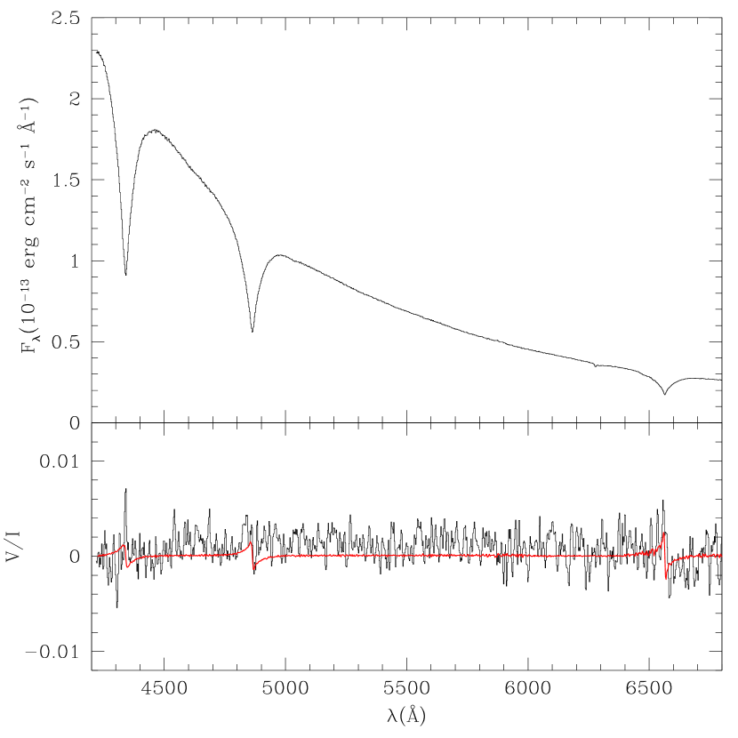
The circular polarization shows a hint of the presence of a weak magnetic field, but the measurement of $-6.1\pm 2.2$ kG does not exceed $3\sigma$ significance. Figure 5 shows the flux and circular polarization spectra of WD 0310$-$688. Note that in a gaussian distribution 0.26% of the objects lie outside $3\sigma$, and therefore the probability that we will have at least one measurement above the $3\sigma$ limit in our sample of 61 white dwarfs is 14.7%. We have checked the individual measurements for each line and we found that the magnetic field at H$\gamma$ was significantly lower and of opposite sign to the measurements obtained at H$\alpha$ and H$\beta$. However, at H$\gamma$ the Zeeman effect is much weaker and the signal-to-noise ratio in this region is much lower. If we only consider the measurements at H$\alpha$ and H$\beta$, then the field measurement would be $-7.3\pm 2.4$, and still barely a $3\sigma$ detection. Aznar Cuadrado et al. (2004) also obtained spectropolarimetry for this star and did not detect the presence of a magnetic field down to a limit of 0.5 kG. Different orientations of the magnetic field as a result of stellar rotation can produce varying field strengths (e.g. WD 0009+501, Valyavin et al., 2005), therefore further spectropolarimetric observations are required to confirm the presence of a magnetic field in WD 0310$-$688.

LB 9802:

This white dwarf is the visual companion to the high-field ultramassive white dwarf, EUVE J0317$-$85.5. We find that the longitudinal field measurement of LB 9802 is $7.2\pm 6.3$ kG, implying that this is a non-magnetic white dwarf. Figure 1 shows the flux and polarization spectra of LB 9802. The magnetic companion EUVE J0317$-$85.5 was found to vary over a 12 minute ($725.4\pm 0.9$ seconds) cycle (Barstow et al., 1995). Using far-ultraviolet spectroscopy Burleigh et al. (1999) found that the magnetic field of EUVE J0317$-$85.5 (RE J0317$-$853) varied between 180 and 800 MG over the surface of the white dwarf assuming a multipolar expansion of the field. Using spectropolarimetry and EUVE photometry (Vennes et al., 2003) were able to improve the period to $725.727\pm 0.001$ seconds. Vennes et al. also suggest that EUVE J0317$-$85.5 has an underlying surface magnetic field of $\sim 185$ MG with a magnetic spot with a surface field strength of $\sim 425$ MG. These two stars have a projected separation of about 200 AU, implying a common origin. However, the more massive star is much hotter than the less massive and cooler LB 9802, which suggests an age disparity between the two stars. A possible explanation for this age disparity is that EUVE J0317$-$85.5 is a result of a double degenerate merger.

WD 0446-789:

This star has recently been observed by Aznar Cuadrado et al. (2004). Using spectropolarimetry they found this white dwarf to have a longitudinal magnetic field of $4.283\pm 0.640$ kG. The detection of a low strength magnetic field in a white dwarf means that a population of low magnetic field white dwarfs may exist. Such a population would contribute toward a wider $B/\Delta B$ distribution shown in Figure 3. Our survey was not sensitive enough to detect fields of a few kG.

WD 0621-376:

Vennes (1999) limited the magnetic field to 30 kG from the narrow H$\alpha$ core. We measured a longitudinal field of $-11.1\pm 10.1$ kG. Assuming that $B_{p}=B_{\ell}/(0.4\cos{i})$ and that $B_{p}=30$ kG, then the longitudinal magnetic field can be at most 12 kG, which clearly lies within $2\sigma$ of our measurement.

WD 0839-327:

This object is a possible double degenerate system (Bragaglia et al., 1990). These authors did not find significant radial velocity changes, however they found significant line profile variations. Using the trigonometric parallax ($\pi=112.7\pm 9.7$ mas) from the Yale Trigonometric Catalog implies a distance of $8.87\pm 0.77$ pc, which is slightly further than the distance obtained from our spectroscopic fit (i.e., 7 pc). Assuming this is a double degenerate, we will assume that the determined parameters (i.e., $T_{\rm eff}=9340$ K and $\log{g}=8.11$) are for the primary (i.e., the brighter component). To approximate the temperature of the secondary component, we first calculate the absolute magnitude of the primary from the temperature and gravity determined from the spectroscopic fit. Therefore, the absolute magnitude of the primary is $M_{V}=12.58$. Next, the total absolute magnitude for the system calculated from the distance ($d=8.9$ pc) and apparent magnitude ($V=11.90$ mag) is $M_{V}=12.15$. The difference in $M_{V}$ suggests that the secondary component would be required to have $M_{V}=13.4$ and assuming $\log{g}=8$ this would correspond to an effective temperature of $\sim 7500$ K.

WD 0859-039:

This star has also been observed by Aznar Cuadrado et al. (2004). Their spectropolarimetric observations did not reveal the presence of a magnetic field in this star down to a limit of $\sim 0.5$ kG, which supports our measurements and non-detection.

WD 1544-377:

This star is the common proper-motion companion to the bright G6V star, HD 140901. Koester et al. (1998) limited the magnetic field to 20 kG from the narrow H$\alpha$ core. We can therefore expect the longitudinal field to be at most 8 kG if we assume a simple dipole for the magnetic field. Both our longitudinal field measurements of $-5.9\pm 7.7$ kG and $-0.25\pm 6.5$ kG lie within 8 kG.

WD 1620-391:

Koester et al. (1998) limited the magnetic field to 10 kG from the narrow H$\alpha$ core, therefore assuming a simple dipole the longitudinal field can be at most 4 kG. We measured a longitudinal field of $-3.0\pm 2.6$ kG and within $2\sigma$ of this measurement we cannot place any tight constraints on the inclination.

WD 1659-531:

This star is the common-proper motion companion to the bright F star, HD 153580. Koester & Herrero (1988) limited the magnetic field to 25 kG from the narrow H$\alpha$ core, and assuming a simple dipole the longitudinal field can be at most 10 kG. We measured a longitudinal field of $-1.1\pm 5.7$ kG and within $2\sigma$ of this measurement we cannot place any tight constraints on the inclination.

WD 2007-303:

Koester et al. (1998) limited the magnetic field to 10 kG from the narrow H$\alpha$ core and assuming a simple dipole the longitudinal field can be at most 4 kG. We have obtained two measurements of the longitudinal field at different epochs ($5.5\pm 8.1$ kG and $3.7\pm 3.8$ kG) which cannot be used to place any tight constraints on the inclination.

WD 2039-682:

A broadened H$\alpha$ core was observed by Koester et al. (1998). They fitted a rotationally broadened profile of $v\sin{i}=80$ km s^-1 to the core, but they also suggested that a magnetic field of $\approx 50$ kG could cause the broadening. Our longitudinal field measurement of $-6.0\pm 6.4$ kG suggests the broadening is most likely due to rotation, however a magnetic field (i.e., $B_{\ell}<12.8$ kG $=2\sigma$) may still be present if it is viewed at high inclination ($i>50^{\circ}$). Also a magnetic spot on the surface of the white dwarf may exist but which was hidden from view when this object was observed during the survey. For example, WD 1953-011 is a known magnetic white dwarf which appears to have a magnetic spot on its surface (Maxted et al., 2000).

WD 2105-820:

Koester et al. (1998) observed a flattened H$\alpha$ core and concluded that it is most likely due to the presence of a magnetic field of $43\pm 10$ kG. Assuming a dipole magnetic field, then the longitudinal field can be at most 17 kG. We measured a longitudinal field of $3.4\pm 5.0$ kG. Within $2\sigma$ of the longitudinal field measurement the inclination has to be greater $39^{\circ}$, however if we consider the uncertainty in the surface field measurement then we cannot constrain the inclination.

WD 2211-495:

This object was discussed in Vennes (1999) who placed an upper limit of 30 kG on the surface magnetic field from the narrow H$\alpha$ core and assuming a simple dipole, the longitudinal field can be at most 12 kG. We measured a longitudinal field of $6.6\pm 5.3$ kG and at $2\sigma$ we cannot place any tight constraints on the inclination of the field.

WD 2359-434

An unusually narrow and flat H$\alpha$ core was reported by Koester et al. (1998) and they speculated that a magnetic field could be the cause of this effect. A variable flattened core was also reported by Maxted & Marsh (1999). A weak magnetic field was detected by Aznar Cuadrado et al. (2004), who measured a lower limit for the longitudinal field strength of $-4.504\pm 0.958$ kG. Our measurement of $3.4\pm 4.4$ kG was not sensitive enough to detect such a low magnetic field. The trigonometric parallax from the Yale Parallax catalog implies a distance of $7.8\pm 0.4$ pc which is in agreement with the distance obtained from the spectroscopic fit.

Table 2 also includes a number of stars that were not observed using spectropolarimetry, but intensity spectra were obtained. We placed an upper limit for the magnetic field of 1MG for these stars. We assumed that the Zeeman splitting would be observed for white dwarfs with surface fields higher than 1 MG. Also we used these optical spectra to determine new effective temperatures and surface gravities for these stars.

In addition, to the above discussed white dwarfs, there are a few objects with peculiar properties that deserve discussion.

WD 0141-675:

This is a known high proper-motion white dwarf, however few spectroscopic observations of this star have been carried out. Holberg et al. (2002) listed this white dwarf as local with a distance of 9.6 pc. Our spectroscopic studies found this object to be a cool white dwarf ($T_{\rm eff}=6460\pm 160$ K) with a distance of 9 pc.

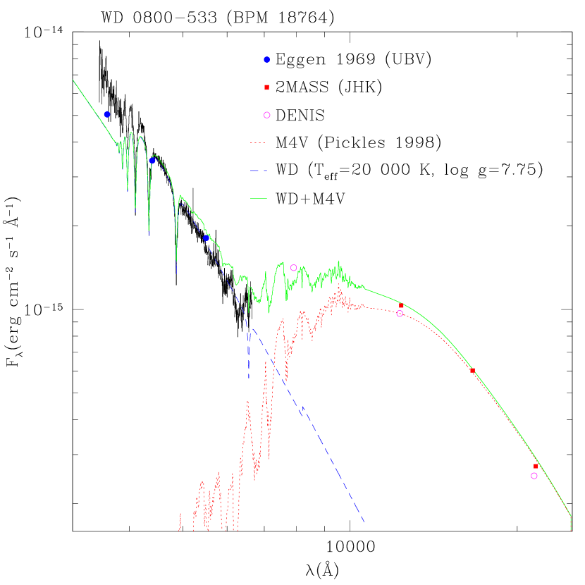
WD 0800-533:

This object was reported as a possible binary by Wickramasinghe & Bessell (1977) who observed broad emission cores in H$\alpha$ and $H\beta$. They also noted that it lies near the X-ray error box of 3U 0804-58. We checked the ROSAT database for X-ray sources in the vicinity of this object, however the closest object is about half a degree away, hence we conclude WD 0800-533 is either not a strong X-ray source or its X-ray emission is variable. Our spectra, which only covers the upper Balmer lines (H$\beta$-H8), did not show obvious signs of emission or a cool companion. However, we obtained 2MASS infrared (JHK) and DENIS (IJK) photometry and found that the white dwarf has significant infrared excess which is possibly due to a cool companion. We estimate the secondary to be a M3-4V star by comparing a combined spectrum of a white dwarf and a M dwarf (Pickles, 1998), as shown in Figure 6. Further studies are required to determine its binary parameters.

Figure 6.— Optical and infrared photometry compared to the observed spectrum of WD 0800-533 and a white dwarf model spectrum ($T_{\rm eff}=20000$ K and $\log{g}=8.0$). Evidence for a cool companion is present with an infrared excess.

WD 1223-659:

This is a local white dwarf ($d\sim 13$ pc) with few spectroscopic observations. Wegner (1973) reported weak Ca II lines, however our spectra only show weak hydrogen lines, in agreement with the classification of Wickramasinghe & Bessell (1977). Therefore, this object is a cool DA white dwarf with $T_{\rm eff}=7740\pm 70$ K and $M=0.67\pm 0.07\ M_{\odot}$.

WD 1236-495:

This is a well known massive ZZ Ceti star. We did not detect the presence of a magnetic field down to about 10 kG. The Balmer lines were fitted with model spectra to obtain an effective temperature of $11870\pm 130$ K and a surface gravity of $\log{g}=8.84\pm 0.04$, and hence a mass of $1.11\pm 0.02M_{\odot}$.

WD 1628-873

has an effective temperature ($T_{\rm eff}=11160\pm 190$ K) and a surface gravity ($\log{g}=8.29\pm 0.07$) that place it near the instability strip. This star was checked for variability by McGraw (1977) who found WD 1628-873 to be constant in luminosity, however it is useful in helping define the instability strip.

WD 2159-754:

This is an ultra-massive white dwarf for which few spectroscopic observations have been carried out. Schulz & Wegner (1981) determined an effective temperature of $T_{\rm eff}=8700\pm 400$ K and a surface gravity $\log{g}=8.1\pm 0.2$ by comparing the equivalent widths of H$\delta/\epsilon$ versus H$\beta/\gamma$. Our surface gravity of $\log{g}=8.95\pm 0.09$ is significantly higher.

WD 2336-079

was observed by Kawka et al. (2004). Their temperature and surface gravity places it in the ZZ Ceti instability strip. Gianninas et al. (2006) have observed this star and found it to be variable. We have re-analyzed this star using improved spectral models and found the effective temperature to be $T_{\rm eff}=11010\pm 210$ K and the surface gravity to be $\log{g}=8.05$ which places this star on the red edge of the instability strip.

WD 2351-368:

This is a high proper-motion white dwarf, and the kinematics of this star make it a halo candidate (Pauli et al., 2003). Halo white dwarfs are expected to be very cool and old, however this star is quite hot ($T_{\rm eff}=14540\pm 320$ K) with an average mass ($M=0.61\pm 0.03M_{\odot}$). Pauli et al. (2003) argue that this white dwarf evolved from a long-lived low mass star. This is one of the few stars for which we could not obtain a spectropolarimetric measurement, and therefore we can only conclude that if a magnetic field is present it must be less than $\sim 1$ MG.

3.2. Ultramassive White Dwarfs

As part of our general spectropolarimetric survey we have also observed EUV-selected ultra-massive ($\geq 1.1\ M_{\odot}$) white dwarfs, which are listed in Tables 1 and 2 and indicated with a tablenote. No magnetic fields were detected in these stars (except for the known magnetic white dwarf EUVE J0823$-$25.4). In addition to the EUV-selected stars, two ultramassive white dwarfs (WD 1236-495 and WD 2159-754) were observed as part of the general survey and were found to be non-magnetic.

Table 5Ultramassive White Dwarfs.

Name	Mass	$B_{p}$	Reference
	($M_{\odot}$)	(MG)
EUVE 0317-855	$1.34\pm 0.03$	450	2
GD 50	$1.27\pm 0.01$	$\lesssim 0.12$	3,4
EUVE 0653-564	$1.16\pm 0.06$	$\lesssim 0.27$	1
EUVE 0823-254	$1.27\pm 0.06$	3.5	1,5
EUVE 1024-303	$1.21\pm 0.05$	$\lesssim 0.12$	1
LTT 4816	$1.11\pm 0.02$	$\lesssim 0.03$	1
EUVE 1535-774	$1.18\pm 0.07$	$\lesssim 0.66$	1
PG 1658+441	$1.31\pm 0.02$	3.5	6,5
EUVE 1727-360	$1.20\pm 0.03$	$\lesssim 0.12$	1
LTT 8816	$1.17\pm 0.03$	$\lesssim 0.03$	1

References. — (1) This work; (2) Ferrario et al. (1997a); (3) Vennes et al. (1997); (4) Schmidt & Smith (1995); (5) Ferrario et al. (1998); (6) Schmidt et al. (1992)

Since the mass of magnetic white dwarfs is on average higher ($\sim 0.8\ M_{\odot}$) than the mass of non-magnetic white dwarfs ($\sim 0.6\ M_{\odot}$) we selected known ultra-massive white dwarfs for which magnetic field measurements are available. Table 3.2 lists these ultra-massive white dwarfs. The presence of a magnetic field is not guaranteed in massive white dwarfs but a higher incidence of magnetism is observed. For the white dwarfs where a magnetic field has been detected, the previously published values are given, otherwise an upper limit on the polar magnetic field from this survey is provided. The upper limit is calculated from the measured $2\sigma$ error of the longitudinal component of the field and since these upper limits are for reference only, we have assumed $57^{\circ}$ for the inclination (i.e., the most probable angle: $\int_{0}^{\pi/2}x\cos{x}dx$).

Figure 7.— Mass distribution of the non-magnetic (see text) and magnetic samples of white dwarfs.

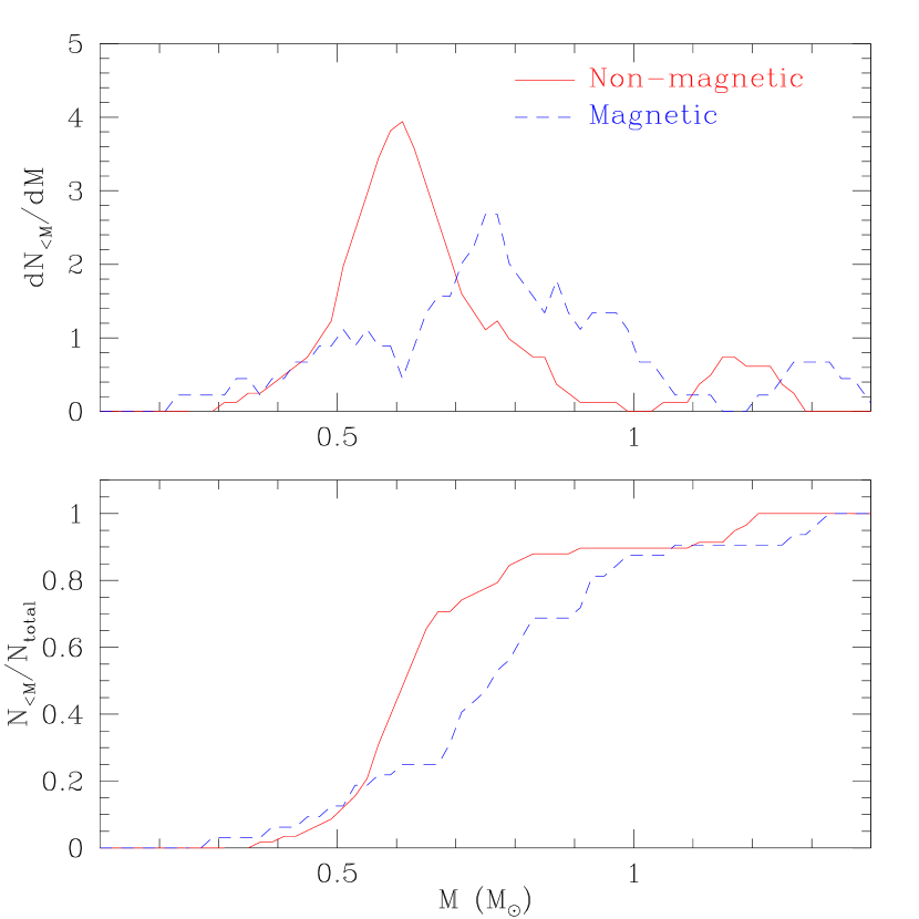
We have calculated the mass distribution of our sample of white dwarfs from Table 2 (excluding the magnetic stars EUVE 0823$-$25.4 and WD 2359-434) and compared it to the mass distribution of magnetic white dwarfs, for which the mass is known. These masses are given in Appendix A. The mass distributions and the cumulative distributions of the non-magnetic and magnetic white dwarfs are shown in Figure 7. The figure shows that magnetic white dwarfs do have higher masses than the non-magnetic white dwarfs. The mean mass of the magnetic white dwarf sample is $\langle M\rangle=0.78\ M_{\odot}$ with a dispersion of $\sigma=0.24\ M_{\odot}$. The mode (i.e., the most probable mass) of the magnetic sample is $0.76\ M_{\odot}$. The mean mass of the non-magnetic sample is $\langle M\rangle=0.68\ M_{\odot}$ with a dispersion of $\sigma=0.20M_{\odot}$. The mode of the non-magnetic sample is $0.57\ M_{\odot}$. If we only consider the major peaks of the two distributions (i.e., excluding the ultramassive white dwarfs), then the mean of the magnetic sample becomes $\langle M\rangle=0.73\ M_{\odot}$ with a dispersion of $\sigma=0.19M_{\odot}$ and the mean of the non-magnetic sample becomes $\langle M\rangle=0.62\ M_{\odot}$ with a dispersion of $\sigma=0.11M_{\odot}$. Wickramasinghe & Ferrario (2005) suggest that the mass distribution is naturally biased toward a higher mass since they assumed high-field magnetic white dwarfs evolve from more massive stars. And the low-field white dwarfs are assumed to evolve from low-mass main-sequence stars which will produce a mass distribution which is similar to that of non-magnetic white dwarfs.

3.2.1 EUVE J0823-25.4

We also observed the massive white dwarf EUVE J0823$-$25.4, shown in Figure 8, which is a known magnetic white dwarf. Ferrario et al. (1998) measured a dipole field of 3.5 MG inclined at a viewing angle of $60^{\circ}$ using the Zeeman split Balmer line profiles. We measured a longitudinal field of $\sim\ -600$ kG. Using the relationship $B_{p}=B_{\ell}/(0.4\cos i$), and B${}_{p}=3.5$ MG, the inclination would be $\sim 65^{\circ}$, which is in agreement with Ferrario et al. (1998).

Figure 8.— The flux (top) and circular polarization (bottom) spectra of the ultra-massive magnetic white dwarf EUVE J0823$-$25.4.

The measurement of the magnetic field at H$\alpha$ resulted in a lower value of $B_{\ell}\sim 63$ kG compared to $\sim 600$ kG for H$\beta$ and H$\gamma$. The H$\alpha$ line profile is dominated by the quadratic Zeeman effect, and the linear Zeeman approximation assumed by the measurement technique is no longer valid and was therefore excluded in calculating the longitudinal field.

3.3. Binary Stars

Table 3 shows the close binaries containing a white dwarf that were observed as part of the survey, giving their apparent magnitude, spectral type, effective temperature and surface gravity.

The spectropolarimetry of BPM 6502 (WD 1042$-$690) suggests the presence of a weak magnetic field. However, because the system is a close binary the Balmer line profiles are shifted between different waveplate exposures. When the final spectra, which have opposite polarization, are subtracted from one another, then the shifted Balmer line profiles can cause the same effect as the shifted $\sigma$ components of the Zeeman effect. Therefore the longitudinal field measurements of close binary systems need to be viewed with caution. Aznar Cuadrado et al. (2004) also observed this system and did not detect the presence of a magnetic field. A similar effect appears to occur for EUVE J0720$-$317. For the close binary LTT 1951, only H$\beta$ and H$\gamma$ were used in the measurement of magnetic field strength. The cool companion dominates the spectrum in the red and therefore H$\alpha$ could not be used in the measurement of the magnetic field of the white dwarf. The measurements we obtained for LTT 1951 indicate that the white dwarf does not possess a strong magnetic field.

Magnetic white dwarfs in binary systems have only been observed in cataclysmic variables or in double degenerate systems such as EUVE 0317$-$855 (Ferrario et al., 1997a) and EUVE 1439$+$750 (Vennes et al., 1999). The distribution of magnetic field strengths of magnetic white dwarfs in cataclysmic variables appears to be similar to the distribution of $B$ of isolated magnetic white dwarfs (Wickramasinghe & Ferrario, 2000). However, there appears to be a paucity of high-field strengths in white dwarfs in cataclysmic variables, which may be a selection effect (Wickramasinghe & Ferrario, 2000). Many magnetic cataclysmic variables are known but no post-common envelope binaries are known to contain a magnetic white dwarf, with the possible exception of SDSS J121209.31+013627.7 (Schmidt et al., 2005) which was found to be a magnetic white dwarf (B${}_{p}=13$ MG) with a probable brown dwarf companion with an orbital period of $\sim 90$ minutes. Liebert (1995) suggested that the reason for the non-detection of magnetic fields in post-common envelope binaries may be due to selection effects, for example the contamination by the secondary spectral features may hide the features that would identify the white dwarf as magnetic. Note that our spectropolarimetric survey of white dwarfs in close binaries with red dwarfs should have easily allowed detection of a field typical in magnetic accretors.

3.4. Non-DA stars

As part of our survey we also observed stars that are non-DA, four of these are sdB stars and one is a DO white dwarf. Table 3 lists these stars and Figure 9 shows their flux and polarization spectra. We did not detect the presence of a magnetic field in any of these stars.

Figure 9.— Flux and circular polarization spectra of the four subdwarfs and one DO white dwarf, which are given in Table 3.)

Two of these stars were misclassified as DA white dwarfs, however the spectra of BPM 36430 and GD 1669 (see also Beers et al., 1992; Lisker et al., 2005) show them to be sdB stars. GD 1669 (WD 2329$-$291) is believed to be magnetic. Koester et al. (1998) observed a broadened H$\alpha$ core in GD 1669 and concluded that it is likely due to presence of a magnetic field of $31\pm 10$ kG. Therefore an upper limit on the longitudinal field would be 12.4 kG, and our measurements ($0.2\pm 5.8$ kG and $7.1\pm 6.7$) clearly lie within this limit. Within $2\sigma$ of the measurements we cannot place any tight constraints on the inclination if a magnetic field of 31 kG is present. Until recently no magnetic fields have been known to exist in sdB stars. O’Toole et al. (2005) have searched for magnetic fields in six sdB/O stars, which resulted in one clear detection of magnetism in HD 76431 and marginal detections in the remaining 5 stars. The broadened Balmer core reported by Koester et al. (1998) may indicate a weak field or it may also suggest that this star is a possible binary (sdB + WD/sdB). More observations of GD 1669 are necessary to determine its status.

For three of the subdwarf B stars effective temperatures and surface gravities have been published, however for BPM 36430, no temperature and surface gravities were found in the available literature. We calculated a grid of LTE line-blanketed spectra for temperatures ranging from 16000 K to 40000 K (in steps of 4000 K), surface gravities between 4.5 to 7.0 (in steps of 0.25 dex) and He-abundances of $\log{(N_{He}/N_{H})}$ = -4 to 0 (in steps of 0.5). We determined the effective temperature, surface gravity and He-abundance for BPM 36430 by fitting the Balmer lines (excluding H$\alpha$) and He lines with synthetic spectra. We found $T_{\rm eff}=30080\pm 660$ K, $\log{g}=5.15\pm 0.16$ and $\log{(N_{He}/N_{H})}\lesssim-3$. The spectrum of BPM 36430 also exhibits NaI and CaII lines. Note that Napiwotzki (1997) found that for sdBs, LTE models begin to deviate from NLTE models above 30000 K, therefore the temperature and gravity of BPM 36430 are probably only slightly lower than our LTE determination.

The magnetic field for the DO white dwarf MCT 0501$-$2858 was measured using 4 helium lines, HeII 4686, HeII 4859, HeII 5412 and HeII 6560. We measured a longitudinal magnetic field of $-5.6\pm 10.4$ kG indicating that the white dwarf does not have a strong magnetic field.

4. Local population of magnetic white dwarfs

Holberg et al. (2002) lists 46 white dwarfs that reside within 13 pc of the Sun, however three of these were found to be F-type stars by Kawka et al. (2004) and need to be removed from the list. Therefore there are 43 known white dwarfs within 13 pc of the Sun of which 9 are magnetic resulting in an incidence of $21\pm 8\%$. Similarly, Holberg et al. (2002) lists 109 white dwarfs residing within 20 pc of the Sun, apart from the three stars already mentioned, the white dwarf WD 1717-345 should be excluded from the list since its distance places it at $\sim 150$ pc. We can add 9 additional stars to the list, eight from Kawka & Vennes (2006) and the newly discovered cool white dwarf PM J13420-3415 from Lepine et al. (2005). Also Zuckerman et al. (2003) found that WD0532+414 and WD0322-019 are double degenerate binaries, therefore we have a total of 116 white dwarfs within 20 pc of the Sun. Of these 15 are classified as magnetic resulting in an incidence of $13\pm 4\%$. The properties of all the known magnetic white dwarfs to date are given in Appendix A.

Figure 10.— Cumulative distributions of magnetic white dwarfs which are with 13 pc (left) and 20 pc (right) of the Sun, compared to a distribution with a constant number per decade interval.

Figure 10 shows the cumulative distribution of magnetic field strengths of white dwarfs found within 13 and 20 pc. A Kolmogorov-Smirnov (KS) test for the white dwarfs within 13 pc shows that the incidence of magnetic white dwarfs appear constant for each decade interval with a probability of 0.7. For the white dwarfs within 20 pc, this probability is reduced to 0.53. The discovery of white dwarfs with kG fields by Aznar Cuadrado et al. (2004) could imply that there is a significant population of white dwarfs with weak magnetic fields.

We have searched the literature for all 116 white dwarfs within 20 pc to find out to what level of magnetic field strength sensitivity each white dwarf has been observed. We have distributed the white dwarfs into four bins which are based on the sensitivity achieved during the observations. Table 6 provides the number of magnetic white dwarfs known in each bin as well as the number of white dwarfs that have been checked for magnetic fields with the corresponding strength for that bin.

Table 6Statistics of magnetism in local white dwarfs.

$B_{p}$	No. of Magnetic WDs	No. of non-magnetic WDs	Fraction
$\geq$ 10 MG	8	14	8/107
1MG - 10 MG	1	31	1/85
100kG - 1 MG	2	18	2/53
$<$ 100 kG	4	29	4/33

Based on these results, we have calculated probabilities in finding more magnetic white dwarfs within 20 pc. In our calculations we have assumed that the $B_{p}$ value of a given bin is a lower limit to which the white dwarfs have been checked, i.e., if a white dwarf has been checked for magnetism down to 1 MG it has also been checked for fields larger than the next bin at 10 MG. We have calculated the probability of finding more magnetic white dwarfs within a given sensitivity bin assuming a binomial probability distribution, i.e.,

$$P(X=x)={n\choose x}p^{x}(1-p)^{n-x}$$ (2)

We calculate the probability ($P$) of finding $x$ number of magnetic white dwarfs in the total number of white dwarfs $n$ that have not been checked for magnetism at the sensitivity level of the given bin. The value of $p$ is determined from the fraction of magnetic white dwarfs in a given bin out of the total number of white dwarfs that have been checked for magnetism in that bin.

In the first bin, 107 out 116 white dwarfs have been checked for magnetic fields greater than or equal to 10 MG. The remaining 9 objects are mostly DC white dwarfs, with one DQ (WD 1043-188). WD 1132-325 (LHS 309) may also be a DQ white dwarf rather than a DC (Henry et al., 2002). There are 8 white dwarfs with measured $B_{p}\geq 10$ MG. Continuum polarization should be detectable in all white dwarfs with $B_{p}\geq 10$ MG. For white dwarfs which display H or He lines, then these lines will be significantly displaced by magnetic fields stronger than 10 MG. Therefore based on the fraction of white dwarfs with $B_{p}\geq 10$ MG ($8/107=0.075$), there is a 50% probability of finding at least one white dwarf with $B_{p}\geq 10$ MG, in the 9 stars.

In the next bin, we have only one magnetic white dwarf (WD 0548-001) and 31 stars that have been checked for magnetic fields between 1 MG and 10 MG. In this bin, white dwarfs showing either H or He lines will display Zeeman splitting and therefore good quality spectroscopy will be sufficient to identify white dwarfs with 1 MG $\leq B_{p}<10$ MG. And we have 23 stars that are not classified as magnetic and have not been checked for magnetism between 1 MG and 10 MG. Therefore, the fraction of white dwarfs with 1 MG $\leq B_{p}<$ 10 MG is 1/85. Assuming that this fraction represents the probability of finding a magnetic white dwarf with a field of 1 MG $\leq B_{p}<$ 10 MG, then the probability that at least one of the 23 white dwarfs (not checked for fields down to 1 MG level) is 0.24. Therefore, it is unlikely that more white dwarfs will be found with 1 MG $\leq B_{p}<$ 10 MG.

In the 100 kG $\leq B_{p}<$ 1 MG bin, again we have two magnetic white dwarfs (WD 0009+501 and WD 0728-642) and 53 stars that have been checked for magnetic fields in this bin. There are 54 stars that are not classified magnetic and have not been checked for magnetism between 100 kG and 1 MG. The fraction of white dwarfs with 100 kG $\leq B_{p}<$ 1 MG is 2/53 and the probability of finding at least one magnetic white dwarf with a field between 100 kG and 1 MG is 0.87 and is therefore a very likely eventuality.

In the final bin ($B_{p}\leq$ 100 kG), we have 4 magnetic white dwarfs (WD 0413-077, WD 1953-011, WD 2105-820 and WD 2359-434) out of 33 stars that have been checked for magnetism at this level. There we can assume that 12% of white dwarfs have magnetic fields below 100 kG. A lower limit to this bin is probably 10 kG, based on the sensitivity of the surveys taken to measure the magnetic field strengths in the 33 stars. There are 72 stars that are not classified as magnetic and that have not been checked for magnetic fields below 100 kG. Note that some of these stars are likely to be in the SPY sample of white dwarfs (Napiwotzki et al., 2001) where magnetic fields less than 100kG would be detectable in the core of the Balmer lines, however since many of the spectra are not yet published we cannot include them in the analysis. The probability that at least one of these stars has a magnetic field less than 100 kG is almost 1. If we calculate the probability of finding a particular number of magnetic white dwarfs in this sample, then the probability peaks at finding 8 white dwarfs $B_{p}\leq 100$ kG among the 72 (P = 0.14). Therefore it is very likely that there are many white dwarfs within 20 pc that have magnetic fields less than 100 kG and the flat distribution of field per decade is probably fortuitous at these low fields.

Figure 11.— Masses and ages for magnetic and non-magnetic white dwarfs within 20pc of the Sun, which were interpolated using relations described in §3.

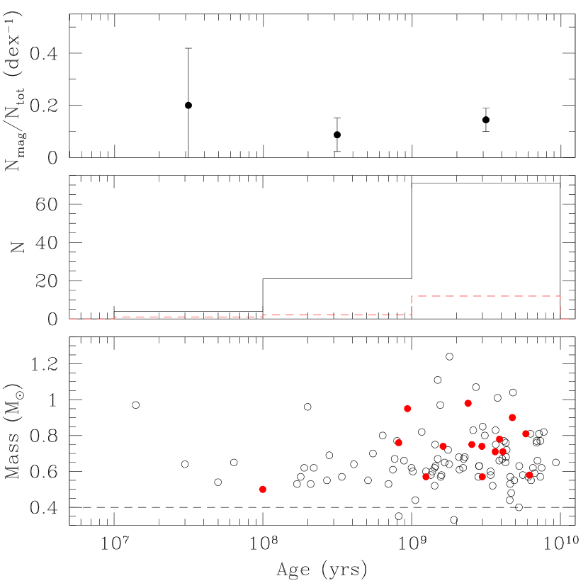
For all the white dwarfs within 20 pc we have obtained the effective temperature, mass and cooling age from the literature. Those for which we could not find a calculated cooling age, we calculated the cooling age using the evolutionary models of Benvenuto & Althaus (1999). For a few white dwarfs we assumed a surface gravity of $\log{g}=8.0$ and hence a mass of $0.57M_{\odot}$. A plot of the mass versus the age for these white dwarfs is shown in Figure 11. The filled circles are the known magnetic white dwarfs within 20 pc and the open circles are the non-magnetic white dwarfs within 20 pc. The plot includes the suspected magnetic white dwarf WD 2105-820 (Koester et al., 1998). Figure 11 also shows the distribution of the cooling age binned into decades, which shows that the local population is relatively old with most white dwarfs having a cooling age greater than $10^{9}$ years. We also calculated the fraction of magnetic white dwarfs for each decade interval of age, which is shown in the top panel of Figure 11. From this plot we can see that there does not appear to be a higher incidence of magnetism among older white dwarfs within the uncertainties of the fractions in each bin. This is in contradiction to other similar studies, such as Liebert et al. (2003a) and Valyavin & Fabrika (1999), which found that the incidence of magnetism is higher in older white dwarfs. In terms of absolute fractions, this appears to be true, but due to the large uncertainty in hot white dwarfs, it is not conclusive, and magnetic incidence may be constant as a function of temperature.

5. Summary

We have conducted a spectropolarimetric survey of southern white dwarfs, which resulted in no new detections of magnetic fields with the possible exception of WD 0310-688 for which we measured a longitudinal field of $-6.1\pm 2.2$ kG. We have also observed the known magnetic white dwarf EUVE J0823-25.4 and measured a longitudinal field of $-600$ kG. However, this survey has helped constrain the incidence of magnetism in the Solar neighborhood. We reviewed the list of known white dwarfs in the Solar neighborhood and found that $21\pm 8\%$ are magnetic. We also investigated the probability of finding more magnetic white dwarfs within the Solar neighborhood based on the current magnetic white dwarf incidence. We found that a significant number of magnetic white dwarfs with fields $B<100$ kG, remain to be detected within the Solar neighborhood.

Appendix A Known Magnetic White Dwarfs

Table Spectropolarimetric survey of hydrogen-rich white dwarf stars lists all the known magnetic white dwarfs as of June 2006. The table gives the WD number, an alternate name, the surface composition of the white dwarf (i.e., whether it is H- or He-rich), the polar magnetic field strength, the effective temperature, the mass of the white dwarf if known, the rotational period if known and references. For a number of white dwarfs, the properties such as the effective temperature and magnetic field strength were determined assuming a surface gravity of $\log{g}=8.0$. For these white dwarfs this is explicitly labeled in the Mass column instead of providing a mass determination.

In Table Spectropolarimetric survey of hydrogen-rich white dwarf stars we list the white dwarfs which have once been classified as magnetic due to their peculiar spectra but which have since been shown to be non-magnetic. The references that show the white dwarf not to be magnetic are provided. Note that the stars are considered non-magnetic at the level advertised in the literature and low-magnetic field in order of kG may still be present in these stars.

Table 7Known Magnetic White Dwarfs.

WD	Other Names	Comp.	$B_{p}$	$T_{\rm eff}$	M	$P_{rot}$	References
			(MG)	(K)	($M_{\odot}$)
0003$-$103	SDSS J000555.91$-$100213.4	He/C	?	29000	$\cdots$	$\cdots$	1,2
0009$+$501	LHS 1038	H	$\lesssim 0.2$	$6540\pm 150$	$0.74\pm 0.04$	$2-20$ hr	3,4
0011$-$134	LHS 1044	H	$16.7\pm 0.6$	$6010\pm 120$	$0.71\pm 0.07$	$\cdots$	5,4
0015$+$004	SDSS J001742.44$+$004137.4	He	8.3	15000	$\cdots$	$\cdots$	1
0018$+$147	SDSS J002129.00$+$150223.7	H	550	7000	$\cdots$	$\cdots$	6
0040$+$000	SDSS J004248.19$+$001955.3	H	14	11000	$\cdots$	$\cdots$	1
0041$-$102	Feige 7	H/He	35	20000	$\log{g}=(8.0)$	131.606 min	7,8
0140$+$130	SDSS J014245.37$+$131546.4	He	4	15000	$\cdots$	$\cdots$	1
0155$+$003	SDSS J015748.15$+$003315.1	He (DZ)	3.7	$\sim 6000$	$\cdots$	$\cdots$	1
0159$-$032	MWD 0159$-$032	H	6	26000	log g = (8.0)	$\cdots$	9
0208$+$002	SDSS J021116.34$+$003128.5	H	490	9000	$\cdots$	$\cdots$	1
0209$+$210	SDSS J021148.22$+$211548.2	H	210	12000	$\cdots$	$\cdots$	6
0233$-$083	SDSS J023609.40$-$080823.9	H(DQA)	5	10000	$\cdots$	$\cdots$	6
0236$-$269	HE 0236$-$2656	He	?	$6000-7000$	$\cdots$	$\cdots$	10
0253$+$508	KPD 0253$+$5052	H	$13-14$	15000	$\log{g}=(8.0)$	$\cdots$	11,12
0257$+$080	LHS 5064	H	$\sim 0.1$	$6680\pm 150$	$0.57\pm 0.09$	$\cdots$	4
0301$-$006	SDSS J030407.40$-$002541.7	H	10.8	15000	$\cdots$	$\cdots$	13
0307$-$428	MWD 0307$-$428	H	10	25000	$\log{g}=(8.0)$	$\cdots$	9
0325$-$857	EUVE J0317$-$855	H	$185-450$	33000	1.35	725 s	14
0329$+$005	KUV 03292$+$0035	H	12.1	26500	$\cdots$	$\cdots$	13
0330$-$000	HE 0330$-$0002	He	?	$6000-7000$	$\cdots$	$\cdots$	10
0340$-$068	SDSS J034308.18$-$064127.3	H	45	13000	$\cdots$	$\cdots$	1
0342$+$004	SDSS J034511.11$+$003444.3	H	1.5	8000	$\cdots$	$\cdots$	13
0413$-$077	40 Eri B	H	$0.0023\pm 0.0007$	$16490\pm 84$	$0.497\pm 0.005$	$\cdots$	15,16
0446$-$789	BPM 3523	H	0.00428	$23450\pm 20$	$0.49\pm 0.01$	$\cdots$	17
0503$-$174	LHS 1734	H	$7.3\pm 0.2$	$5300\pm 120$	$0.37\pm 0.07$	$\cdots$	5,4
0548$-$001	G 99$-$37	C2/CH	$\sim 10$	$6070\pm 100$	$0.69\pm 0.02$	4.117 hr	18,19,20
0553$+$053	G 99$-$47	H	$20\pm 3$	$5790\pm 110$	$0.71\pm 0.03$	0.97 hr	21,4,20
0616$-$649	EUVE J0616$-$649	H	14.8	50000	$\log{g}=(8.0)$	$\cdots$	22
0637$+$477	GD 77	H	$1.2\pm 0.2$	$14870\pm 120$	0.69	$\cdots$	23,24
0728$+$642	G 234$-$4	H	$0.0396\pm 0.0116$	$4500\pm 500$	$\cdots$	$\cdots$	25
0745$+$304	SDSS J074850.48$+$301944.8	H	10	22000	$\cdots$	$\cdots$	6
0755$+$358	SDSS J075819.57$+$354443.7	H	27	22000	$\cdots$	$\cdots$	1
0756$+$437	G 111$-$49	H	220	$8500\pm 500$	$\cdots$	$\cdots$	26,25
0801$+$186	SDSS J080440.35$+$182731.0	H	49	11000	$\cdots$	$\cdots$	6
0802$+$220	SDSS J080502.29$+$215320.5	H	5	28000	$\cdots$	$\cdots$	6
0804$+$397	SDSS J080743.33$+$393829.2	H	49	13000	$\cdots$	$\cdots$	1
0806$+$376	SDSS J080938.10$+$373053.8	H	40	14000	$\cdots$	$\cdots$	6
0814$+$043	SDSS J081648.71$+$041223.5	H	10:	11500	$\cdots$	$\cdots$	6
0816$+$376	GD 90	H	9	14000	$\log{g}=(8.0)$	$\cdots$	27,25
0821$-$252	EUVE J0823$-$254	H	$2.8-3.5$	$43200\pm 1000$	$1.20\pm 0.04$	$\cdots$	28
0825$+$297	SDSS J082835.82$+$293448.7	H	30	19500	$\cdots$	$\cdots$	6
0837$+$199	EG 61	H	$\sim 3$	$17100\pm 350$	$0.817\pm 0.032$	$\cdots$	29
0837$+$273	SDSS J084008.50$+$271242.7	H	10	12250	$\cdots$	$\cdots$	6
0839$+$026	SDSS J084155.74$+$022350.6	H	6	7000	$\cdots$	$\cdots$	1
0843$+$488	SDSS J084716.21$+$484220.4	H	$\sim 3$	19000	$\cdots$	$\cdots$	1
0853$+$163	LB 8915	H/He	$0.75-1.0$	24000	$\log{g}=(8.0)$	$\cdots$	30
0855$+$416	SDSS J085830.85$+$412635.1	H	2	7000	$\cdots$	$\cdots$	1
0903$+$083	SDSS J090632.66$+$080716.0	H	10	17000	$\cdots$	$\cdots$	6
0904$+$358	SDSS J090746.84$+$353821.5	H	15	16500	$\cdots$	$\cdots$	6
0908$+$422	SDSS J091124.68$+$420255.9	H	45	10250	$\cdots$	$\cdots$	6
0911$+$059	SDSS J091437.40$+$054453.3	H	9.5	17000	$\cdots$	$\cdots$	6
0912$+$536	G 195$-$19	He	$\sim 100$	$7160\pm 190$	$0.75\pm 0.02$	1.3301 d	31,4,32
0922$+$014	SDSS J092527.47$+$011328.7	H	2.2	10000	$\cdots$	$\cdots$	1
0930$+$010	SDSS J093313.14$+$005135.4	He (C2H)?	?	$\cdots$	$\cdots$	$\cdots$	1
0931$+$105	SDSS J093356.40$+$102215.7	H	1.5	8500	$\cdots$	$\cdots$	6
0931$+$507	SDSS J093447.90$+$503312.2	H	9.5	8900	$\cdots$	$\cdots$	6
0941$+$458	SDSS J094458.92$+$453901.2	H	14	15500	$\cdots$	$\cdots$	6
0945$+$246	LB 11146	H	670	$16000\pm 2000$	$0.90^{+0.10}_{-0.14}$	$\cdots$	33,34
0952$+$094	SDSS J095442.91$+$091354.4	DQ	?	$\cdots$	$\cdots$	$\cdots$	6
0957$+$022	SDSS J100005.67$+$015859.2	H	20	9000	$\cdots$	$\cdots$	1
1001$+$058	SDSS J100356.32$+$053825.6	H	900	23000	$\cdots$	$\cdots$	6
1004$+$128	SDSS J100715.55$+$123709.5	H	7	18000	$\cdots$	$\cdots$	6
1008$+$290	LHS 2229	He (C2H)	$\sim 100$	4600	$\cdots$	$\cdots$	35
1012$+$093	SDSS J101529.62$+$090703.8	H	5	7200	$\cdots$	$\cdots$	6
1013$+$044	SDSS J101618.37$+$040920.6	H	7.5	10000	$\cdots$	$\cdots$	1
1015$+$014	PG 1015$+$014	H	$120\pm 10$	14000	$\log{g}=(8.0)$	98.74734 min	36,37,38
1017$+$367	GD 116	H	$65\pm 5$	16000	$\cdots$	$\cdots$	39
1026$+$117	LHS 2273	H	18	$7160\pm 170$	(0.59)	$\cdots$	40
1031$+$234	PG 1031$+$234	H	$\sim 200-1000$	$\sim 15000$	$\cdots$	3.3997 hr	41,42,43
1033$+$656	SDSS J103655.38$+$652252.0	DQ	4:	$\cdots$	$\cdots$	$\cdots$	1
1036$-$204	LP 790$-$29	He	50	7800	$\log{g}=(8.0)$	$24-28$ d	44,45
1043$-$050	HE 1043$-$0502	He	$\sim 820$	$\sim 15000$	$\cdots$	$\cdots$	46,10
1045$-$091	HE 1045$-$0908	H	16	$10000\pm 1000$	$\log{g}=(8.0)$	$2.7$ hr	47
1050$+$598	SDSS J105404.38$+$593333.3	H	17	9500	$\cdots$	$\cdots$	1
1053$+$656	SDSS J105628.49$+$652313.5	H	28	16500	$\cdots$	$\cdots$	1
1105$-$048	LTT 4099	H	0.0039	$15280\pm 20$	$0.52\pm 0.01$	$\cdots$	17
1107$+$602	SDSS J111010.50$+$600141.4	H	6.5	30000	$\cdots$	$\cdots$	1
1111$+$020	SDSS J111341.33$+$014641.7	He ?	?	$\cdots$	$\cdots$	$\cdots$	1
1115$+$101	SDSS J111812.67$+$095241.4	H	6	10500	$\cdots$	$\cdots$	6
1126$-$008	SDSS J112852.88$-$010540.8	H	3	11000	$\cdots$	$\cdots$	1
1126$+$499	SDSS J112924.74$+$493931.9	H	5	10000	$\cdots$	$\cdots$	6
1131$+$521	SDSS J113357.66$+$515204.8	H	7.5	22000	$\cdots$	$\cdots$	1
1135$+$579	SDSS J113756.50$+$574022.4	H	9	7800	$\cdots$	$\cdots$	6
1136$-$015	LBQS 1136$-$0132	H	$24\pm 1$	10500	$\cdots$	$\cdots$	48,1
1137$+$614	SDSS J114006.37$+$611008.2	H	58	13500	$\cdots$	$\cdots$	1
1145$+$487	SDSS J114829.00$+$482731.2	H	33	27500	$\cdots$	$\cdots$	6
1151$+$015	SDSS J115418.14$+$011711.4	H	32	27000:	$\cdots$	$\cdots$	1
1156$+$619	SDSS J115917.39$+$613914.3	H	15.5	23000	$\cdots$	$\cdots$	1
1159$+$619	SDSS J120150.10$+$614257.0	H	20	10500	$\cdots$	$\cdots$	6
1203$+$085	SDSS J120609.80$+$081323.7	H	830:	13000	$\cdots$	$\cdots$	6
1204$+$444	SDSS J120728.96$+$440731.6	H	2.5	16750	$\cdots$	$\cdots$	6
1209$+$018	SDSS J121209.31$+$013627.7	H	13	10000	$\cdots$	$\cdots$	1
1211$-$171	HE 1211$-$1707	He	50	$\sim 12000$	$\cdots$	$\sim 2$ hr	10
1212$-$022	LHS 2534	He(DZ)	1.92	6000	$\cdots$	$\cdots$	49
1214$-$001	SDSS J121635.37$-$002656.2	H	63	20000	$\cdots$	$\cdots$	13
1219$+$005	SDSS J122209.44$+$001534.0	H	12	20000	$\cdots$	$\cdots$	13
1220$+$484	SDSS J122249.14$+$481133.1	H	8	9000	$\cdots$	$\cdots$	6
1220$+$234	PG 1220$+$234	H	3	26540	0.81	$\cdots$	37
1221$+$422	SDSS J122401.48$+$415551.9	H	23:	9500	$\cdots$	$\cdots$	6
1231$+$130	SDSS J123414.11$+$124829.6	H	7	8200	$\cdots$	$\cdots$	6
1245$+$413	SDSS J124806.38$+$410427.2	H	8	7000	$\cdots$	$\cdots$	6
1246$-$022	SDSS J124851.31$-$022924.7	H	7	13500	$\cdots$	$\cdots$	1
1248$+$161	SDSS J125044.42$+$154957.4	H	20	10000	$\cdots$	$\cdots$	6
1252$+$564	SDSS J125416.01$+$561204.7	H	52	13250	$\cdots$	$\cdots$	6
1254$+$345	HS 1254$+$3440	H	$9.5\pm 0.5$	$15000\pm 4000$	$\cdots$	$\cdots$	50
1309$+$853	G 256$-$7	H	$4.9\pm 0.5$	$\sim 56000$	$\cdots$	$\cdots$	26
1312$+$098	PG 1312$+$098	H	10	$\sim 20000$	$\cdots$	5.42839 hr	38,25
1317$+$135	SDSS J132002.48$+$131901.6	H	5	14750	$\cdots$	$\cdots$	6
1327$+$594	SDSS J132858.20$+$590851.0	H	18	25000	$\cdots$	$\cdots$	6
1328$+$307	G165-7	He (DZ)	0.65	$6440\pm 210$	$0.57\pm 0.17$	$\cdots$	51
1330$+$015	G 62$-$46	H	$7.36\pm 0.11$	6040	0.25	$\cdots$	52
1331$+$005	SDSS J133359.86$+$001654.8	He (C2H) ?	?	$\cdots$	$\cdots$	$\cdots$	1
1332$+$643	SDSS J133340.34$+$640627.4	H	13	13500	$\cdots$	$\cdots$	1
1339$+$659	SDSS J134043.10$+$654349.2	H	3	15000	$\cdots$	$\cdots$	1
1349$+$545	SBS 1349$+$5434	H	760	11000	$\cdots$	$\cdots$	53
1350$-$090	LP 907$-$037	H	$\lesssim 0.3$	$9520\pm 140$	$0.83\pm 0.03$	$\cdots$	54,55
1425$+$375	SDSS J142703.40$+$372110.5	H	30	19000	$\cdots$	$\cdots$	6
1430$+$432	SDSS J143218.26$+$430126.7	H	30	24000	$\cdots$	$\cdots$	6
1430$+$460	SDSS J143235.46$+$454852.5	H	30	16750	$\cdots$	$\cdots$	6
1440$+$753	EUVE J1439$+$750	H	$14-16$	$20000-50000$	$0.88-1.19$	$\cdots$	56
1444$+$592	SDSS J144614.00$+$590216.7	H	7	12500	$\cdots$	$\cdots$	1
1452$+$435	SDSS J145415.01$+$432149.5	H	5	11500	$\cdots$	$\cdots$	6
1503$-$070	GD 175	H	2.3	6990	$0.70\pm 0.13$	$\cdots$	4
1506$+$399	SDSS J150813.20$+$394504.9	H	20	17000	$\cdots$	$\cdots$	6
1509$+$425	SDSS J151130.20$+$422023.0	H	12	9750	$\cdots$	$\cdots$	6
1516$+$612	SDSS J151745.19$+$610543.6	H	17	9500	$\cdots$	$\cdots$	1
1531$-$022	GD 185	H	$0.035\pm 0.016$	$18620\pm 285$	$0.88\pm 0.03$	$\cdots$	55,57
1533$+$423	SDSS J153532.25$+$421305.6	H	4.5	18500	$\cdots$	$\cdots$	1
1533$-$057	PG 1533$-$057	H	$31\pm 3$	$20000\pm 1040$	$0.94\pm 0.18$	$\cdots$	58,11,55
1537$+$532	SDSS J153829.29$+$530604.6	H	12	13500	$\cdots$	$\cdots$	1
1539$+$039	SDSS J154213.48$+$034800.4	H	8	8500	$\cdots$	$\cdots$	1
1603$+$492	SDSS J160437.36$+$490809.2	H	53	9000	$\cdots$	$\cdots$	1
1639$+$537	GD 356	He	13	$7510\pm 210$	$0.67\pm 0.07$	0.0803 d	59,4,60
1641$+$241	SDSS J164357.02$+$240201.3	H	4	16500	$\cdots$	$\cdots$	6
1645$+$372	SDSS J164703.24$+$370910.3	H	2:	16250	$\cdots$	$\cdots$	6
1648$+$342	SDSS J165029.91$+$341125.5	H	3:	9750	$\cdots$	$\cdots$	6
1650$+$355	SDSS J165203.68$+$352815.8	H	9.5	11500	$\cdots$	$\cdots$	1
1658$+$440	PG 1658$+$440	H	$2.3\pm 0.2$	$30510\pm 200$	$1.31\pm 0.02$	$\cdots$	61
1702$+$322	SDSS J170400.01$+$321328.7	H	5	23000	$\cdots$	$\cdots$	6
1713$+$393	NLTT 44447	H	1.3	6260	$\cdots$	$\cdots$	62
1715$+$601	SDSS J171556.29$+$600643.9	H	4.5	13500	$\cdots$	$\cdots$	6
1719$+$562	SDSS J172045.37$+$561214.9	H	21	22500	$\cdots$	$\cdots$	13
1722$+$541	SDSS J172329.14$+$540755.8	H	33	16500	$\cdots$	$\cdots$	13
1728$+$565	SDSS J172932.48$+$563204.1	H	28	10500	$\cdots$	$\cdots$	1
1743$-$520	BPM 25114	H	36	$\sim 20000$	$\log{g}=(8.0)$	2.84 d	63,64
1748$+$708	G 240$-$72	He	$\gtrsim 100$	$5590\pm 90$	$0.81\pm 0.01$	$\gtrsim 20$ yr	18,4,65
1814$+$248	G 183$-$35	H	$\sim 14$	$6500\pm 500$	$\log{g}=(8.0)$	$\sim 50$ min $-$ few yr	26,25
1818$+$126	G 141$-$2	H	$\sim 3$	$6340\pm 130$	$0.26\pm 0.12$	$\cdots$	66,40
1829$+$547	G 227$-$35	H	$170-180$	$6280\pm 140$	$0.90\pm 0.07$	$\cdots$	21,4
1900$+$705	Grw $+70^{\circ}8247$	H	$320\pm 20$	16000	$0.95\pm 0.02$	$\cdots$	67,68,4
1953$-$011	G 92$-$40	H	$0.1-0.5$	$7920\pm 200$	$0.74\pm 0.03$	1.44176 d	69,4,70
2010$+$310	GD 229	He	$520$	18000	$\log{g}=(8.0)$	$\cdots$	46
2043$-$073	SDSS J204626.15$-$071037.0	H	2	8000	$\cdots$	$\cdots$	1
2049$-$004	SDSS J205233.52$-$001610.7	H	13	19000	$\cdots$	$\cdots$	1
2105$-$820	L 24$-$52	H	$0.043\pm 0.01$ ?	$10200\pm 290$	$0.75\pm 0.03$	$\cdots$	57,4
2146$+$005	SDSS J214900.87$+$004842.8	H	10	11000	$\cdots$	$\cdots$	6
2146$-$077	SDSS J214930.74$-$072812.0	H	42	22000	$\cdots$	$\cdots$	1
2149$+$002	SDSS J215135.00$+$003140.5	H	$\sim 300$	9000	$\cdots$	$\cdots$	1
2149$+$126	SDSS J215148.31$+$125525.5	H	21	14000	$\cdots$	$\cdots$	1
2215$-$002	SDSS J221828.59$-$000012.2	H	225	15500	$\cdots$	$\cdots$	1
2245$+$146	SDSS J224741.46$+$145638.8	H	560	18000	$\cdots$	$\cdots$	1
2316$+$123	KUV 813$-$14	H	$45\pm 5$	$11000\pm 1000$	$\log{g}=(8.0)$	17.856 d	21,38
2317$+$008	SDSS J231951.73$+$010909.3	H	1.5:	8300	$\cdots$	$\cdots$	6
2320$+$003	SDSS J232248.22$+$003900.9	H	13	39000	$\cdots$	$\cdots$	13
2321$-$010	SDSS J232337.55$-$004628.2	He	4.8	15000	$\cdots$	$\cdots$	1
2329$+$267	PG 2329$+$267	H	$2.31\pm 0.59$	$9400\pm 240$	$0.61\pm 0.16$	$\cdots$	71,4
2343$+$386	SDSS J234605.44$+$385337.7	H	1000	26000	$\cdots$	$\cdots$	6
2343$-$106	SDSS J234623.69$-$102357.0	H	2.5	8500	$\cdots$	$\cdots$	6
2359$-$434	LTT 9857	H	0.0031	$8570\pm 50$	$0.98\pm 0.04$	$\cdots$	17,72

References. — (1) Schmidt et al. (2003); (2) Liebert et al. (2003b); (3) Valyavin et al. (2005); (4) Bergeron et al. (2001); (5) Bergeron et al. (1992); (6) Vanlandingham et al. (2005); (7) Achilleos et al. (1992); (8) Liebert et al. (1977); (9) Achilleos et al. (1991); (10) Schmidt et al. (2001); (11) Achilleos & Wickramasinghe (1989); (12) Friedrich et al. (1997); (13) Gänsicke et al. (2002); (14) Vennes et al. (2003); (15) Fabrika et al. (2000); (16) Finley et al. (1997); (17) Aznar Cuadrado et al. (2004); (18) Angel (1978); (19) Dufour et al. (2005); (20) Pragal & Bues (1989) (21) Putney & Jordan (1995); (22) Vennes (1999); (23) Schmidt et al. (1992); (24) Giovannini et al. (1998); (25) Putney (1997) (26) Putney (1995); (27) Martin & Wickramasinghe (1984); (28) Ferrario et al. (1998); (29) Claver et al. (2001); (30) Wesemael et al. (2001); (31) Angel (1977); (32) Angel et al. (1972); (33) Glenn et al. (1994); (34) Liebert et al. (1993); (35) Schmidt et al. (1999); (36) Wickramasinghe & Cropper (1988); (37) Liebert et al. (2003a); (38) Schmidt & Norsworthy (1991); (39) Saffer et al. (1989); (40) Bergeron et al. (1997); (41) Latter et al. (1987); (42) 0̈streicher et al. (1992); (43) Schmidt et al. (1986); (44) Bues (1999); (45) Jordan & Friedrich (2002); (46) Wickramasinghe et al. (2002); (47) Euchner et al. (2005); (48) Foltz et al. (1989); (49) Reid et al. (2001); (50) Hagen et al. (1987); (51) Dufour et al. (2006); (52) Bergeron et al. (1993); (53) Liebert et al. (1994); (54) Schmidt & Smith (1994); (55) Liebert et al. (2005); (56) Vennes et al. (1999); (57) Koester et al. (1998); (58) Liebert et al. (1985); (59) Ferrario et al. (1997b); (60) Brinkworth et al. (2004); (61) Schmidt et al. (1992); (62) Kawka & Vennes (2006); (63) Wickramasinghe & Martin (1979); (64) Wegner (1977); (65) Berdyugin & Piirola (1999); (66) Greenstein (1986); (67) Wickramasinghe & Ferrario (1988); (68) Jordan (1992); (69) Maxted et al. (2000); (70) Brinkworth et al. (2005); (71) Moran et al. (1998); (72) This work

Table 8Stars removed from previous lists of magnetic white dwarfs.

WD	Other Names	Spectral Type	$T_{\rm eff}$	M	References
			(K)	($M_{\odot}$)
0000$-$345	HE 0000$-$3430	DC	$6240\pm 140$	$0.77\pm 0.11$	1,2
0003$-$570	HE 0003$-$5701	DA $+$ dMe	$\gtrsim 80000$	$\cdots$	1
0026$-$218	HE 0026$-$2150	DA $+$ dMe	$\cdots$	$\cdots$	1
0107$-$019	HE 0107$-$0158	DA $+$ dMe	$\cdots$	$\cdots$	1
0127$-$311	HE 0127$-$3110	DZ (?)	$\cdots$	$\cdots$	1
0136$+$251	PG 0136$+$251	DA	$39400\pm 1200$	$1.24\pm 0.04$	3,4
0338$-$388	HE 0338$-$3853	DA $+$ dMe	$87000-97000$	$\cdots$	1
2201$-$228	HE 2201$-$2250	DB	$\cdots$	$\cdots$	5

References. — (1) Schmidt et al. (2001); (2) Bergeron et al. (2001); (3) Schmidt et al. (1992); (4) Vennes (1999); (5) Jordan (2001)

References

- Achilleos et al. (1991) Achilleos, N., Remillard, R.A. & Wickramasinghe, D.T. 1991, MNRAS, 253, 522
- Achilleos & Wickramasinghe (1989) Achilleos, N. & Wickramasinghe, D.T. 1989, ApJ, 346, 444
- Achilleos et al. (1992) Achilleos, N., Wickramasinghe, D.T., Liebert, J., Saffer, R.A., & Grauer, A.D. 1992, ApJ, 396, 273
- Angel (1977) Angel, J.R.P. 1977, ApJ, 216, 1
- Angel (1978) Angel, J.R.P. 1978, ARA&A, 16, 487
- Angel et al. (1981) Angel, J.R.P., Borra, E.F., & Landstreet, J.D. 1981, ApJS, 45, 457
- Angel et al. (1972) Angel, J.R.P., Illing, R.M.E. & Landstreet, J.D. 1972, ApJ, 175, L85
- Angel et al. (1973) Angel, J.P.R., McGraw, J.T., & Stockman, H.S. 1973, ApJ, 184, L79
- Aznar Cuadrado et al. (2004) Aznar Cuadrado, R., Jordan, S., Napiwotzki, R., Schmid, H.M., Solanki, S.K., & Mathys, G. 2004, A&A, 423, 1081
- Barstow et al. (1995) Barstow, M.A., Jordan, S., O’Donoghue, D., Burleigh, M.R., Napiwotski, R., & Harrop-Allin, M.K. 1995, MNRAS, 277, 971
- Beers et al. (1992) Beers, T.C., Preston, G.W., Shectman, S.A., Doinidis, S.P., & Griffin, K.E. 1992, AJ, 103, 267
- Benvenuto & Althaus (1999) Benvenuto, O.G., & Althaus, L.G. 1999, MNRAS, 303, 30
- Berdyugin & Piirola (1999) Berdyugin, A.V. & Piirola, V. 1999, A&A, 352, 619
- Bergeron et al. (1992) Bergeron, P., Ruiz, M.T., & Leggett, S.K. 1992, ApJ, 400, 315
- Bergeron et al. (1992b) Bergeron, P., Wesemael, F., & Fontaine, G. 1991, ApJ, 387, 288
- Bergeron et al. (1993) Bergeron, P., Ruiz, M.T., & Leggett, S.K. 1993, ApJ, 407, 733
- Bergeron et al. (1997) Bergeron, P., Ruiz, M.T., & Leggett, S.K. 1997, ApJS, 108, 339
- Bergeron et al. (2001) Bergeron, P., Leggett, S.K., & Ruiz, M.T. 2001, ApJS, 133, 413
- Bragaglia et al. (1990) Bragaglia, A., Greggio, L., Renzini, A., & D’Odorico, S. 1990, ApJ, 365, L13
- Bragaglia et al. (1995) Bragaglia, A., Renzini, A., & Bergeron, P. 1995, ApJ, 443, 735
- Brinkworth et al. (2004) Brinkworth, C.S., Burleigh, M.R., Wynn, G.A., & Marsh, T.R. 2004, MNRAS, 348, L33
- Brinkworth et al. (2005) Brinkworth, C.S., Marsh, T.R., Morales-Rueda, L., Maxted, P.F.L., Burleigh, M.R., & Good, S.A. 2005, MNRAS, 357, 333
- Bues (1999) Bues, I. 1999, 11th European Workshop on White Dwarfs, eds. J.-E. Solheim & E.G. Meistas, ASP Conf. Ser. 169 (San Francisco CA: ASP), 240
- Burleigh et al. (1999) Burleigh, M.R., Jordan, S. & Schweizer, W. 1999, ApJ, 510, L37
- Claver et al. (2001) Claver, C.F., Liebert, J., Bergeron, P. & Koester, D. 2001, ApJ, 563, 987
- Cohen et al. (1993) Cohen, M.H., Putney, A. & Goodrich, R.W. 1993, ApJ, 405, L67
- Dufour et al. (2005) Dufour, P., Bergeron, P., & Fontaine, G. 2005, ApJ, 627, 404
- Dufour et al. (2006) Dufour, P., Bergeron, P., Schmidt, G.D., Liebert, J., Harris, H.C., Knapp, G.R., Anderson, S.F. & Schneider, D.P. 2006, ApJ, in press (astro-ph/0608065)
- Euchner et al. (2005) Euchner, F., Reinsch, K., Jordan, S., Beuermann, K., & Gänsicke, B.T. A&A, 442, 651
- Fabrika et al. (2000) Fabrika, S., Valyavin, G., Burlakova, T.E., Barsukova, E.A. and Monin, D.N. 2000, Magnetic Fields of Chemically Peculiar and Related Stars, ed. Yu.V. Glogolevskij & I.I. Romanyuk, 218
- Ferrario et al. (1998) Ferrario, L., Vennes, S., Wickramasinghe, D.T. 1998, MNRAS, 299, L1
- Ferrario et al. (1997a) Ferrario, L., Vennes, S., Wickramasinghe, D.T., Bailey, J.A., Christian, D.T. 1997a, MNRAS, 292, 205
- Ferrario et al. (1997b) Ferrario, L., Wickramasinghe, D.T., Liebert, J., Schmidt, G.D. & Bieging, J.H. 1997b, MNRAS, 289, 105
- Finley et al. (1997) Finley, D.S., Koester, D. & Basri, G. 1997, ApJ, 488, 375
- Foltz et al. (1989) Foltz, C.B., Latter, W.B., Hewett, P.C., Weymann, R.J., Morris, S.L. & Anderson, S.F. 1989, AJ, 98, 665
- Fontaine et al. (1981) Fontaine, G., Villeneuve, B., & Wilson, J. 1981, ApJ, 627, 404
- Friedrich et al. (1997) Friedrich, S., König, M., & Schweizer, W. 1997, A&A, 326, 218
- Gänsicke et al. (2002) Gänsicke, B.T., Euchner, F. & Jordan, S. 2002, A&A, 394, 957
- Gianninas et al. (2006) Gianninas, A., Bergeron, P., & Fontaine, G. 2006, AJ, accepted (astro-ph/0606135)
- Giovannini et al. (1998) Giovannini, O., Kepler, S.O., Kanaan, A., Wood, M.A., Claver, C.F. & Koester, D. 1998, Baltic Astronomy, 7, 131
- Glenn et al. (1994) Glenn, J., Liebert, J. & Schmidt, G.D. 1994, PASP, 106, 722
- Greenstein (1986) Greenstein, J.L. 1986, ApJ, 194, L51
- Hagen et al. (1987) Hagen, H.-J., Groote, D., Engles, D., Haug, U., Toussaint, F. & Reimer, D. 1987, A&A, 183, L7
- Henry et al. (2002) Henry, T.J., Walkowicz, L.M., Barto, T.C., & Golimowski, D.A. 2002, AJ, 123, 2002
- Holberg et al. (2002) Holberg, J.B., Oswalt, T.D., & Sion, E.M. 2002, ApJ, 571, 512
- Hubeny et al. (1994) Hubeny, I., Hummer, D.G., & Lanz, T. 1994, A&A, 282, 151
- Hummer & Mihalas (1988) Hummer, D.G., & Mihalas, D. 1988, ApJ, 331, 794
- Jordan (1992) Jordan, S. 1992, A&A, 265, 570
- Jordan (2001) Jordan, S. 2001, 12th European Workshop on White Dwarfs, eds. J.L. Provencal, H.L. Shipman, J. MacDonald & S. Goodchild, ASP Conf. Ser. 226 (San Francisco CA: ASP), 269
- Jordan & Friedrich (2002) Jordan, S. & Friedrich, S. 2002, A&A, 383, 519
- Jordan et al. (1998) Jordan, S., Schmelcher, P., Becken, W., & Schweizer, W. 1998, A&A, 336, L33
- Kawka (2004) Kawka, A. 2004, PhD (Thesis), ’A Study of White Dwarfs in the Solar Neighbourhood’, Murdoch University
- Kawka & Vennes (2004) Kawka, A., & Vennes, S. 2004, in IAU Symposium 224: The A-Star Puzzle, ed. J. Zverko, J. Ziznovsky, S.J. Adelman, & W.W. Weiss Cambridge Uni. Press, 879
- Kawka & Vennes (2006) Kawka, A., & Vennes, S. 2006, ApJ, 643, 402
- Kawka et al. (2004) Kawka, A., Vennes, S., & Thorstensen, J.R. 2004, AJ, 127, 1702
- Kawka et al. (2003) Kawka, A., Vennes, S., Wickramasinghe, D.T., Schmidt, G.D., & Koch, R. 2003, in White Dwarfs, ed. D. de Martino, J.E. Solheim & R. Kalytis, Kluwer Academic Publishers. NATO Science Series II, 105, 179
- Kemp (1970) Kemp, J.C. 1970, ApJ, 162, 169
- Koester et al. (1998) Koester, D., Dreizler, S., Weidemann, V., & Allard, N.F. 1998, A&A, 338, 612
- Koester & Herrero (1988) Koester, D. & Herrero, A. 1988, ApJ, 332, 910
- Latter et al. (1987) Latter, W.B., Schmidt, G.D. & Green, R.F. 1987, ApJ, 320, 308
- Lemke (1997) Lemke, M. 1997, A&AS, 122, 285
- Lepine et al. (2005) Lepine, S., Rich, R.M., & Shara, M.M. 2005, ApJ, 633, L121
- Liebert (1995) Liebert, J. 1995, in ASP Conf. Ser. 85, Cape Workshop on Magnetic Cataclysmic Variables, ed. D.A.H. Buckley & B. Warner (San Francisco: ASP), 59
- Liebert et al. (1977) Liebert, J. Angel, J.R.P., Stockman, H.S., Spinrad, H., & Beaver, E.A. 1997, ApJ, 214, 457
- Liebert et al. (2003a) Liebert, J., Bergeron, P., & Holberg, J.B. 2003b, AJ, 125, 348
- Liebert et al. (2005) Liebert, J., Bergeron, P., & Holberg, J.B. 2005, ApJS, 156, 47
- Liebert et al. (1993) Liebert, J., Bergeron, P., Schmidt, G.D. & Saffer, R.A. 1993, ApJ, 1993, 418, 426
- Liebert et al. (2003b) Liebert, J., et al. 2003b, AJ, 126, 2521
- Liebert et al. (1994) Liebert, J., Schmidt, G.D., Lesser, M., Stepanian, J.A., Lipovetsky, V.A., Chaffe, F.H. & Foltz, C.B. 1994, ApJ, 421, 733
- Liebert et al. (1985) Liebert, J., Schmidt, G.D., Sion, E.M., Starrfield, S.G., Green, R.F. & Boroson, T.A. 1985, PASP, 97, 158
- Lisker et al. (2005) Lisker, T., Heber, U., Napiwotzki, R., Christlieb, N., Han, Z., Homeier, D., & Reimers, D. 2005, A&A, 430, 223
- Martin & Wickramasinghe (1984) Martin, B. & Wickramasinghe, D.T. 1984, MNRAS, 206, 407
- Maxted et al. (2000) Maxted, P.F.L., Ferrario, L., Marsh, T.R. & Wickramasinghe, D.T. 2000, MNRAS, 315, L41
- Maxted & Marsh (1999) Maxted, P.F.L. & Marsh, T.R. 1999, MNRAS, 307, 122
- McGraw (1977) McGraw, J.T. 1977, ApJ, 214, L123
- Mihalas (1978) Mihalas, D. 1978, Stellar Atmospheres, 2nd Ed. (San Francisco: Freeman)
- Moran et al. (1998) Moran, C., Marsh, T.R. & Dhillon, V.S. 1998, MNRAS, 299, 218
- Napiwotzki (1997) Napiwotzki, R. 1997, A&A, 322, 256
- Napiwotzki et al. (2001) Napiwotzki, R., et al. 2001, Astronomische Nachrichten, 322, 411
- O’Donoghue et al. (1998) O’Donoghue, D., Koen, C., Lynas-Gray, A.E., Kilkenny, D., & van Wyk, F. 1998, MNRAS, 296, 306
- 0̈streicher et al. (1992) 0̈streicher, R., Seifer, W., Friedrich, S., Ruder, H., Schaich, M., Wolf, D. & Wunner, G. 1992, A&A, 257, 353
- O’Toole et al. (2005) O’Toole, S.J., Jordan, S., Friedrich, S., & Heber, U. 2005, A&A, 437, 227
- Pauli et al. (2003) Pauli, E.-M., Napiwotzki, R., Altmann, M., Heber, U., Odenkirchen, M., & Ferber, F. 2003, A&A, 400, 877
- Pickles (1998) Pickles, A.J. 1998, PASP, 110, 863
- Pragal & Bues (1989) Pragal, M. & Bues, I. 1989, Astronomische Gesellschaft Abstract Series, 45
- Putney (1997) Putney, A. 1997, ApJS, 112, 527
- Putney (1995) Putney, A. 1995, ApJ, 451, L67
- Putney & Jordan (1995) Putney, A. & Jordan, S. 1995, ApJ, 449, 863
- Reid et al. (2001) Reid, I.N., Liebert, J., & Schmidt, G.D. 2001, ApJ, 550, L61
- Saffer et al. (1989) Saffer, R.A., Liebert, J., Wagner, R.M., Sion, E.M. & Starrfield, S.G. 1989, AJ, 98, 668
- Schmidt et al. (1992) Schmidt, G.D., Bergeron, P., Liebert, J. & Saffer, R.A. 1992, ApJ, 394, 603
- Schmidt et al. (2003) Schmidt, G.D., et al. 2003, ApJ, 595, 1101
- Schmidt et al. (1999) Schmidt, G.D., Liebert, J., Harris, H.C., Dahn, C.C. & Leggett, S.K. 1999, ApJ, 512, 916
- Schmidt & Norsworthy (1991) Schmidt, G.D. & Norsworthy, J.E. 1991, ApJ, 366, 270
- Schmidt & Smith (1995) Schmidt, G.D. & Smith, P.S. 1995, ApJ, 448, 305
- Schmidt & Smith (1994) Schmidt, G.D. & Smith, P.S. 1994, ApJ, 423, L63
- Schmidt et al. (1992) Schmidt, G.D., Stockman, H.S. & Smith, P.S. 1992, ApJ, 398, L57
- Schmidt et al. (2005) Schmidt, G.D., Szkody, P., Silvestri, N.M., Cushing, M.C., Liebert, J., & Smith, P.S. 2005, ApJ, 630, L173
- Schmidt et al. (2001) Schmidt, G.D., Vennes, S., Wickramasinghe, D.T. & Ferrario, L. 2001, MNRAS, 328, 203
- Schmidt et al. (1986) Schmidt, G.D., West, S.C., Liebert, J., Green, R.F. & Stockman, H.S. 1986, ApJ, 309, 218
- Schulz & Wegner (1981) Schulz, H., & Wegner, G. 1981, A&A, 94, 272
- Valyavin et al. (2005) Valyavin, G., Bagnulo, S., Monin, D., Fabrika, S. Lee, B.-C., Galazutdinov, G., Wade, G.A., & Burlakova, T. 2005, A&A, 439, 1099
- Valyavin & Fabrika (1999) Valyavin, G., & Fabrika , S. 1999, 11th European Workshop on White Dwarfs, eds. J.-E. Solheim & E.G. Meistas, ASP Conf. Ser. 169 (San Francisco CA: ASP), 206
- Vanlandingham et al. (2005) Vanlandingham, K.M., et al. 2005, AJ, 130, 734
- Vennes (1999) Vennes, S. 1999, ApJ, 525, 995
- Vennes et al. (1998) Vennes, S., Dupuis, J., Chayer, P., Polomski, E.F., Dixon, W.V., & Hurwitz, M. 1998, ApJ, 500, L41
- Vennes et al. (1999) Vennes, S., Ferrario, L., & Wickramasinghe, D.T. 1999, MNRAS, 302, L49
- Vennes et al. (2003) Vennes, S., Schmidt, G.D., Ferrario, L., Christian, D.J., Wickramasinghe, D.T., & Kawka, A. 2003, ApJ, 593, 1040
- Vennes et al. (1997) Vennes, S., Thejll, P.A., Galvan, R.G., & Dupuis, J. 1997, ApJ, 480, 714
- Vennes et al. (1996) Vennes, S., Thejll, P.A., Wickramasinghe, D.T., & Bessell, M.S. 1996, ApJ, 467, 782
- Wegner (1973) Wegner, G. 1973, MNRAS, 163, 381
- Wegner (1977) Wegner, G. 1977, Memorie Societa Astronomica Italiana, 48, 27
- Wesemael et al. (2001) Wesemael, F., Liebert, J., Schmidt, G.D., Beauchamp, A., Bergeron, P. & Fontaine, G. 2001, ApJ, 554, 1118
- Wickramasinghe & Bessell (1977) Wickramasinghe, D.T. & Bessell, M.S. 1977, MNRAS, 181, 713
- Wickramasinghe & Cropper (1988) Wickramasinghe, D.T. & Cropper, M. 1988, MNRAS, 235, 1451
- Wickramasinghe & Ferrario (1988) Wickramasinghe, D.T. & Ferrario, L. 1988, ApJ, 327, 222
- Wickramasinghe & Ferrario (2000) Wickramasinghe, D.T. & Ferrario, L. 2000, PASP, 112, 873
- Wickramasinghe & Ferrario (2005) Wickramasinghe, D.T. & Ferrario, L. 2005, MNRAS, 356, 1576
- Wickramasinghe & Martin (1979) Wickramasinghe, D.T. & Martin, B. 1979, MNRAS, 235, 1451
- Wickramasinghe et al. (2002) Wickramasinghe, D.T., Schmidt, G.D., Ferrario, L. & Vennes, S. 2002, MNRAS, 332, 29
- Wood (1995) Wood, M.A. 1995, in White Dwarfs, ed. D. Koester & K. Werner (New York: Springer), 41
- Zuckerman et al. (2003) Zuckerman, B., Koester, D., Reid, I.N., & Hünsch, M. 2003, ApJ, 596, 477