Optical and X-Ray Observations of GRB 060526: A Complex Afterglow Consistent with An Achromatic Jet Break

Abstract

We obtained 98 $R$-band and 18 $B$, $r^{\prime}$, $i^{\prime}$ images of the optical afterglow of GRB 060526 ($z=3.21$) with the MDM 1.3m, 2.4m, and the PROMPT telescopes in Cerro Tololo over the 5 nights following the burst trigger. Combining these data with other optical observations reported in GCN and the Swift-XRT observations, we compare the optical and X-ray afterglow light curves of GRB 060526. Both the optical and X-ray afterglow light curves show rich features, such as flares and breaks. The densely sampled optical observations provide very good coverage at $T>10^{4}$ sec. We observed a break at $2.4\times 10^{5}$ sec in the optical afterglow light curve. Compared with the X-ray afterglow light curve, the break is consistent with an achromatic break supporting the beaming models of GRBs. However, the pre-break and post-break temporal decay slopes are difficult to explain in simple afterglow models. We estimated a jet angle of $\theta_{j}\sim 7^{\circ}$ and a prompt emission size of $R_{prompt}\sim 2\times 10^{14}$ cm. In addition, we detected several optical flares with amplitudes of $\Delta m\sim 0.2$, 0.6, and 0.2 mag. The X-ray afterglows detected by Swift have shown complicated decay patterns. Recently, many well-sampled optical afterglows also show decays with flares and multiple breaks. GRB 060526 provides an additional case of such a complex, well observed optical afterglow. The accumulated well-sampled afterglows indicate that most of the optical afterglows are complex.

1 Introduction

In the fireball model (Mészáros & Rees, 1997; Sari et al., 1998), the afterglow emission of gamma-ray bursts (GRBs) are thought to be synchrotron emission in the external shocks. After the launch of Swift (Gehrels et al., 2004), with its rapid localization of GRBs and the dedicated on-board XRT instrument, the afterglow models can be tested extensively with the regularly obtained XRT light curves. More than half of the Swift-XRT light curves show complicated decay patterns with multiple breaks and giant X-ray flares (Burrows et al., 2005; Nousek et al., 2006; O’Brien et al., 2006). New ingredients were added to the models to interpret these features (e.g., Zhang et al., 2006; Nousek et al., 2006; Panaitescu et al., 2006a). Compared with the large number of Swift-XRT afterglows, only a few bursts have good optical afterglow coverage, which limits the multi-wavelength study of GRB afterglows. Moreover, a large fraction of the well-studied optical afterglows also show complicated behaviors (e.g., Guidorzi et al. 2005; Blustin et al. 2006; Rykoff et al. 2006; Stanek et al. 2006), challenging the simple, smooth-decay afterglow models.

Another important aspect of the models is that GRBs are thought to be collimated in jets, based on the achromatic breaks observed in many optical GRB afterglow light curves (e.g., Stanek et al., 1999). Different jet models have been proposed for GRBs either under a uniform jet model (e.g., Rhoads, 1999; Frail et al., 2001; Granot et al., 2002) or a structured jet model (e.g., Lipunov et al., 2001; Zhang & Mészáros, 2002; Rossi et al., 2002; Lloyd-Ronning et al., 2004; Zhang et al., 2004; Dai & Zhang, 2005). Some of these jet models can also unify the closely related phenomena of X-ray flashes with GRBs (Yamazaki et al., 2003; Zhang et al., 2004; Lamb et al., 2005; Dai & Zhang, 2005). Since the distinct signature that a jet imposes on GRB afterglow light curves (an achromatic break) is simply a geometric effect, it is important to test the wavelength independence across the broadest possible wavelength range, for example between optical and X-ray afterglow light curves. To date, the lack of wavelength dependence has only been confirmed across different optical bands. Recently, GRB 050525A (Blustin et al., 2006), GRB 050801 (Rykoff et al., 2006), and GRB 060206 (Stanek et al., 2006) show possible achromatic breaks across optical and X-ray light curves. However, in GRB 050801, the break is interpreted as energy injection or the onset of the afterglow, and in GRB 060206, it is debated whether the break is achromatic (Monfardini et al., 2006).

As many XRT light curves show multiple breaks, it is not obvious which of them should be associated with the optical break and which of them interpreted as the jet break. Recently, Panaitescu et al. (2006b); Fan & Piran (2006) showed that some of the X-ray breaks (1–4 hours after the burst trigger) are chromatic from X-rays to optical bands. However, as the X-ray light curves have several breaks, it is possible that the achromatic jet break occurs at some later time. In addition, as many optical afterglows also show rich features such as flares and multiple breaks (e.g., Stanek et al. 2006), fits to poorly sampled optical light curves may not be reliable.

In this paper, we report the optical follow-up of GRB 060526 with the MDM 1.3m, 2.4m telescopes and the PROMPT at Cerro Tololo, and our detection of an achromatic break across the optical and X-ray bands. GRB 060526 was detected by the BAT on board Swift at 16:28:30 UT on May 26, 2006 (Campana et al. 2006). The XRT and UVOT rapidly localized the burst location. The burst was followed up with ground-based telescopes by several groups. In particular, Berger & Gladders (2006) reported the burst redshift of $z=3.21$. We organize the paper as follows. First, we describe the data reduction in §2. In §3, we describe the evolution of the GRB afterglow and perform a comparison between the optical and X-ray light curves. Finally, we discuss our results in §4.

2 The Optical and X-ray Data Reduction

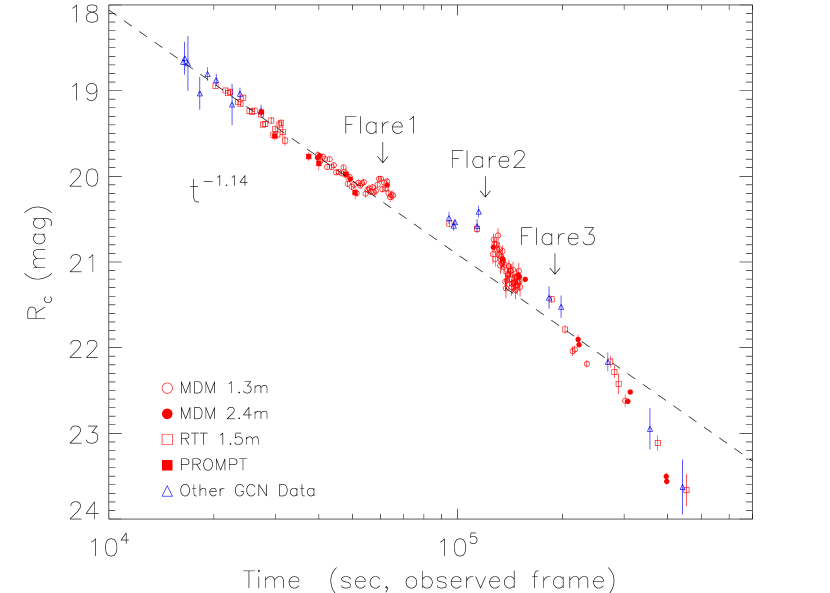
Figure 2: The densely sampled optical light curve from $10^{4}$ sec after the burst trigger. The open circles, filled circles, and fill squares are our MDM 1.3m, 2.4m, and PROMPT observations and the rest of the data are from GCN circulars. The data before $5.4\times 10^{4}$ sec is fitted by a power-law with a slope of $1.14\pm 0.02$ (dashed line). Compared with the single power-law fit, the late optical data clearly show multiple flares and a much steeper late time decay slope of $3.4\pm 0.2$.

We obtained 83 and 15 optical $R$-band exposures with the MDM 1.3m, 2.4m telescopes, and 18 $B$, $r^{\prime}$, $i^{\prime}$ images with the PROMPT in Cerro Tololo, respectively, on the nights of 26-30 May 2006. After standard bias subtraction and flatfielding, we measured relative fluxes between GRB 060526 and six nearby reference stars that had been calibrated using the Landolt (1992) standard field on the 1.3m. The local reference stars also served to tie the 2.4m data onto the 1.3m photometric system, with typical rms scatter of the 2.4m zeropoint determination of 0.02-0.03 magnitudes for each epoch. In general, overlapping GRB 060526 data between the two telescopes agreed to within the computed error bars (see Fig. 2). As GRB 060526 was a bright burst observed by many groups, we also collected other R-band observations reported in the GCN circulars (French & Jelinek, 2006; Covino et al., 2006; Lin et al., 2006; Khamitov et al., 2006a, b, c, d, e, f; Rumyantsev et al., 2006a, b; Kann & Hoegner, 2006; Baliyan et al., 2006; Terra et al., 2006). When the reference stars and their magnitudes were given, we calibrated their magnitudes to our magnitude system.

We also reduced the Swift-XRT data for GRB 060526. The XRT observations cover 6 days with gaps in between for the burst. We analyzed the XRT level 2 event files for both the windowed timing (WT) and photon counting (PC) modes. These events were filtered to be within 0.2-10 keV energy band and restricted to grades of 0–2 for the WT mode and 0–12 for the PC mode. We extracted the XRT spectra and light-curves with the software tool xselect . We use the rmf files from the standard XRT calibration distribution, and generated the arf files with the Swift-XRT software tool . Finally, we fit the X-ray spectra with XSPEC (Arnaud, 1996).

3 Evolution of the Afterglow

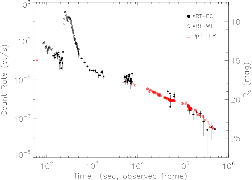
Figure 1: X-ray and optical afterglow light curves of GRB 060526. The open and filled circles are data from the XRT Windowed Timing mode and Photon Counting mode, respectively, and the red squares are the R band optical data from our MDM 1.3m, 2.4m, and PROMPT observations combined with other optical observations reported in the GCN. The normalization between the optical and X-ray light curves is $f_{o}/f_{x}\sim 1000$ for the late afterglow light curve ($T>3\times 10^{4}$ sec), and the optical to X-ray spectral index is $\beta_{ox}\sim 1.0$.

The overall optical and X-ray light-curves of GRB 060526 are shown in Fig. 1, and data are listed in Tables 1 and 2. In addition, we also show the densely sampled optical data in more detail in Fig. 2. Both the optical and X-ray light curves exhibit rich features including flares and breaks beyond a simple power-law decay. Below, we discuss the evolution of the optical and X-ray light curves separately at first and then compare them afterward. Following the literature, we model the segments of the afterglow with single power-laws of $f_{\nu}\propto t^{-\alpha}\nu^{-\beta}$. We also used the broken power-law for the temporal decay in some cases as $f(t)\propto((\frac{t}{t_{b}})^{\alpha_{e}s}+(\frac{t}{t_{b}})^{\alpha_{l}s})^{-1/s}$, where $\alpha_{e}$, $\alpha_{l}$, $t_{b}$, and $s$ are the early and late decay indices, break time, and smoothness parameters, respectively. We fixed the smoothness parameter to $s=2.5$ for our analysis.

The optical light curve shows at least one break at $T\sim 2.4\times 10^{5}$ sec and possibly an earlier one at $T\sim 10^{4}$ sec. In addition, we detect multiple optical flares in our densely sampled regions. The light curve between $10^{4}<T<5.4\times 10^{4}$ sec is well fitted by a power-law with a slope of $1.14\pm 0.02$ (Fig. 2). In the period between $5.4\times 10^{4}<T<2.0\times 10^{5}$ sec, several optical flares occurred, based on the shape of the light curve and the extrapolation of the power-law decay slope from the previous stage. The flares peak at $\sim 6.1\times 10^{4}$, $1.2\times 10^{5}$, and $1.8\times 10^{5}$ sec with peak magnitude changes of $\Delta m\sim 0.2,0.6$, and $0.2$ mag, respectively, above a power-law extrapolation from the previous period, and the durations of flares, $\Delta t$, are $1.4\pm 0.5\times 10^{4}$ sec, $9\pm 2\times 10^{4}$ sec, and $4\pm 2\times 10^{4}$ sec. After the flares, the light curve steepens ($T>2.4\times 10^{5}$ sec) as a power-law, and we find an index of $3.4\pm 0.2$, assuming that the optical flares do not contribute to this part of the light curve. If we treat the optical afterglow light curve as the “bump and wiggle” modification of the smooth afterglow instead of flares on top of a smooth afterglow, we fit all the optical data points ($T>10^{4}$ sec) with a broken power-law and we find early and late decay slopes of $\sim 1.0$ and $\sim 2.9$ and a break time at $\sim 2.2\times 10^{5}$ sec. This fit is statistically unacceptable because it cannot describe the “bump and wiggle” part of the afterglow. We estimated the optical spectral index from the $B,r^{\prime},i^{\prime}$ images taken by the PROMPT close to $4\times 10^{4}$ sec and obtained $\beta_{o}=1.69^{+0.53}_{-0.49}$ (Fig. 3). We have taken account of the effects from Galactic extinction and the Ly$\alpha$ forest.

The most striking features of the X-ray light curve are the two X-ray flares between 225 and 600 sec after the burst trigger. We find that the flares peak at $T=250$ sec and $T=300$ sec after the trigger, consistent with the GCN report (Campana et al., 2006b). If we neglect the data points dominated by the two X-ray flares, the light curve can be fitted with several power-law segments, as with many other XRT afterglow light curves observed with Swift (Nousek et al., 2006) and theoretical models (Zhang et al., 2006). Besides the breaks and the two giant flares, the X-ray light curve also shows small amplitude variability between $5000<T<8000$ sec and possibly between $4\times 10^{4}<T<6.4\times 10^{4}$ sec. The XRT light curve decays as $\alpha_{1}=2.3\pm 0.2$ at $T<225$ sec before the flares. After the two X-ray flares, the X-ray emission decays slowly with $\alpha_{2}\sim 0.5$ between $850<T<8000$ sec. The extrapolation of the shallow decay slope does not fit the remaining data point, and the rest of the afterglow evolution is expected to follow the “normal+jet” decay stage. However, the exact time of the transition is unknown because of the gaps in the XRT light curve. If we assume the transition occurs at between $5000<T<8000$ sec and fit the data points at $T>5000$ sec with a broken power-law model, we obtained $\alpha_{3}\sim 1.1$, $\alpha_{4}\sim 3.3$, and $T_{b}\sim 2.3\times 10^{5}$ sec. We also fitted the X-ray light curve after the two giant flares ($T>850$ sec) using a single break and obtained a good fit with $\alpha_{2}\sim 0.5$, $\alpha_{3}\sim 1.6$, and $T_{b}\sim 2\times 10^{4}$ sec. Essentially, this is equivalent to replacing the previous “normal+jet” model with a single power-law decay of slope 1.6. Finally, we analyzed the X-ray spectra of the GRB afterglow for several stages and show the evolution in Fig. 3. We detected spectral evolution before and after the two X-ray flares. After the X-ray flares, we found the X-ray spectral indices are roughly consistent except that the index for the shallow decay stage ($\alpha_{2}\sim 0.5$) is slightly harder.

The late optical light curve ($T>10^{4}$ sec) clearly shows a break at $2.4\times 10^{5}$ sec, while the X-ray light curve can be modeled both as a broken power-law and single power-law. If the X-ray light curve decays as a single power-law at this stage, it obviously does not follow the optical afterglow. On the other hand, the fitting results of the broken power-law model for the X-ray light curve are similar to those obtained from optical data. Given the signal-to-noise of the late X-ray data and possible contamination from flares, it is difficult to distinguish the two models from the X-ray data alone. Instead, since the properties of the optical afterglow are better constrained, we raise the question whether the X-ray afterglow is consistent with the best fit optical model. The fitting results show that they are consistent, i.e., the optical and X-ray data are consistent with an achromatic broken power-law model with superimposed flares.

4 Discussion

We present well-sampled optical and X-ray afterglow light curves of GRB 060526. As discussed in the previous section, the evolution of the afterglow is complicated with multiple breaks and flares both in the optical and the X-ray bands. The combination of flares and incomplete data sampling present severe challenges to measuring the temporal decay slopes of the afterglow, even for a well-sampled burst such as GRB 060526. Below, we proceed by assuming that our analysis results are not significantly affected by these factors.

We detected a possible achromatic jet break in the optical and X-ray afterglow light curves. Before this late-time break ($T\sim 2.4\times 10^{5}$ sec), the afterglow is consistent with many Swift afterglows (Nousek et al., 2006). The X-ray light curve started with a steep decay ($\alpha_{1}=2.3\pm 0.2$), which is interpreted as the tail of the prompt emission due to the “curvature effect” (Kumar & Panaitescu, 2000). The spectral and temporal indices are constrained as $\alpha=\beta+2$, which is consistent with the X-ray spectral index of $\beta_{1}=0.55\pm 0.15$. The X-ray light curve then entered into a shallow decay stage with $\alpha_{2}\sim 0.5$, which we interpret as energy injection. Then it decays into a normal afterglow stage with $\alpha_{3}=1.14\pm 0.02$ as constrained from the optical observations. In addition, the X-ray light curve shows two huge flares which are commonly seen in Swift X-ray afterglows and are attributed to late time central engine activities. After the achromatic break, the afterglow enters a very steep stage with $\alpha_{4}=3.4\pm 0.2$. The X-ray and optical-to-X-ray spectral indices after $5000$ sec are consistent with $\sim 1$, suggesting that the optical and X-ray bands are on the same power-law segment of the spectral energy distribution. The optical spectral index is marginally consistent with the X-ray index, although the error-bar is large.

The achromatic break observed in optical afterglows is traditionally interpreted as the jet break. As mentioned in the introduction, the achromatic break is not yet confirmed across optical and X-ray light curves. Here, we present a case in GRB 060526 where such an achromatic break is observed across the optical and X-ray afterglows, supporting the beaming model of the GRBs. However, the afterglow decay slopes before and after the break are hard to reconcile with simple afterglow-jet models. The late time decay slope after the jet break should follow $\alpha=p$ (Sari et al., 1999), where $p$ is power-law index for the electrons $N(\gamma)\propto\gamma^{-p}$. The post-jet slope, $3.4\pm 0.2$, is too steep for a pre-jet slope of $1.14\pm 0.02$ under any combination of either constant or wind medium and relative positions between $\nu$, $\nu_{m}$, and $\nu_{c}$. Since the achromatic break is most easily explained by a jet, it is possible that more complicated afterglow models are needed (e.g., Panaitescu et al., 2006b) with non-standard micro-physical parameters. Another possibility is that energy injection or flares continued contributing significant flux and significantly affected the temporal decay slope. We estimated the jet angle (half opening angle for uniform jets or observer’s viewing angle for structured jets) using $t_{j}\simeq 6.2(E_{52}/n)^{1/3}(\theta_{j}/0.1)^{8/3}$ hr (Sari et al., 1999) and obtained $\theta_{j}\sim 7^{\circ}$ assuming ambient density $n=1~{}$cm^-3. We further estimated the size of the $\gamma$-ray prompt emission by combining the measured jet angle and the X-ray tail emission detected before 225 sec using $t_{tail}=(1+z)(R_{prompt}/c)(\theta_{j}^{2}/2)$ (Zhang et al., 2006) and obtained $R_{prompt}\sim 2\times 10^{14}$ cm.

We also observed multiple optical flares in the light curve of GRB 060526. Optical flares or re-brightenings have been observed in both pre-Swift (e.g., GRB 970508, GRB 021004, and GRB 030329, Galama et al., 1998; Lazzati et al., 2002; Bersier et al., 2003; Mirabal et al., 2003; Lipkin et al., 2004) and Swift bursts (e.g., GRB 050525A, GRB 050820A, GRB 060206, GRB 060210, GRB 060605, GRB 060607, and GRB 061007, Blustin et al., 2006; Cenko et al., 2006; Stanek et al., 2006; Schaefer et al., 2006; Nysewander et al., 2006; Bersier et al., 2006). The fraction of bursts with optical flares seemed small. However, recently many well-sampled bursts show complex optical decay behaviors. The accumulating observations argue that it is possible that most of optical afterglows are complex and the appearance of simplicity was a consequence of poor sampling. There are several interpretations for the optical flares, such as models of density fluctuations, “patchy shell”, “refreshed shock”, and late central engine activities (e.g., Jakobsson et al., 2004; Ioka et al., 2005; Gorosabel et al., 2006). We estimated the quantities $\Delta t/t=0.23\pm 0.08$, $0.75\pm 0.17$, and $0.22\pm 0.11$ and $\Delta F_{\nu}/F_{\nu}\sim 0.2$, 0.7, and 0.2, respectively, for the three flares detected in GRB 060526. The $\Delta t/t$ values are small which do not favor the models of patchy shell and refreshed shock, since the model predictions are $\Delta t/t>1$ and $>1/4$ for these two models (Ioka et al., 2005). The properties of the flares barely satisfy Ioka et al.’s constraint, $\Delta F_{\nu}/F_{\nu}<1.6\Delta t/t$, under the density fluctuation model. Recently, Nakar & Granot (2006) also modeled the effects of density fluctuations on the afterglow light curves and found that they cannot produce the sharp features observed in many bursts. Another possibility is that the flares (or breaks) indicate the onset of the afterglow (Rykoff et al., 2006; Stanek et al., 2006) scaled with the isotropic energy as $T_{onset}\propto E_{iso}^{1/3}$ (Sari, 1997). The onset time also depends on the density of the ambient medium and the initial Lorentz factor that are more difficult to measure. We might expect a correlation between $E_{iso}$ and $T_{onset}$ for a large sample of bursts, or if the densities and Lorentz factors for the bursts only spread in a narrow range. We tested this hypothesis by plotting the two properties for bursts with optical flares in Fig. 4, and did not detect positive correlation between the two properties. However, we notice the difference between flares that occur before the optical afterglow has decayed and those that occur afterward. The flares in GRB 050820A, GRB 060210, GRB 060605, GRB 060607, and GRB 061007 possibly belong to the category of flares that occur before the afterglow has faded, and they roughly follow the scaling between isotropic energy and flare time. However, a larger sample is needed to fully test the model. In any case, the flares in GRB 060526 are unlikely to be associated with the onset of the afterglow. It is possible that these flares are from late central engine activities, which can have arbitrary variabilities. However, we are open to other theoretical models which can be tested extensively with our well-sampled light curve.

Table 1: Optical Light Curves of GRB 060526.

Telescope	Time	Band	Magnitude
	(sec)
MDM 1.3m	39744	R	19.75$\pm$0.04
MDM 1.3m	40349	R	19.83$\pm$0.04
MDM 1.3m	41040	R	19.77$\pm$0.03
MDM 1.3m	41645	R	19.80$\pm$0.03
MDM 1.3m	42250	R	19.89$\pm$0.03
MDM 1.3m	42941	R	19.80$\pm$0.03
MDM 1.3m	43546	R	19.89$\pm$0.03
MDM 1.3m	44150	R	19.87$\pm$0.03
MDM 1.3m	44842	R	19.95$\pm$0.04
MDM 1.3m	45619	R	19.95$\pm$0.03
MDM 1.3m	46483	R	19.97$\pm$0.03
MDM 1.3m	47088	R	19.90$\pm$0.03
MDM 1.3m	47779	R	19.97$\pm$0.03
MDM 1.3m	48384	R	20.09$\pm$0.04
MDM 1.3m	49075	R	20.01$\pm$0.03
MDM 1.3m	49680	R	20.12$\pm$0.04
MDM 1.3m	50458	R	20.10$\pm$0.04
MDM 1.3m	51322	R	20.20$\pm$0.04
MDM 1.3m	51926	R	20.08$\pm$0.04
MDM 1.3m	52531	R	20.11$\pm$0.04
MDM 1.3m	53222	R	20.08$\pm$0.04
MDM 1.3m	53827	R	20.07$\pm$0.04
MDM 1.3m	54432	R	20.20$\pm$0.04
MDM 1.3m	55123	R	20.16$\pm$0.04
MDM 1.3m	55728	R	20.14$\pm$0.04
MDM 1.3m	56333	R	20.18$\pm$0.04
MDM 1.3m	57024	R	20.13$\pm$0.04
MDM 1.3m	57629	R	20.19$\pm$0.04
MDM 1.3m	58234	R	20.17$\pm$0.04
MDM 1.3m	58925	R	20.10$\pm$0.04
MDM 1.3m	59530	R	20.03$\pm$0.04
MDM 1.3m	60221	R	20.03$\pm$0.04
MDM 1.3m	60826	R	20.15$\pm$0.04
MDM 1.3m	61430	R	20.07$\pm$0.04
MDM 1.3m	62122	R	20.14$\pm$0.04
MDM 1.3m	62726	R	20.06$\pm$0.04
MDM 1.3m	63331	R	20.20$\pm$0.05
MDM 1.3m	64022	R	20.24$\pm$0.06
MDM 1.3m	64627	R	20.22$\pm$0.05
MDM 1.3m	65232	R	20.22$\pm$0.06
MDM 1.3m	126230	R	20.91$\pm$0.11
MDM 1.3m	126835	R	20.74$\pm$0.07
MDM 1.3m	127526	R	20.79$\pm$0.07
MDM 1.3m	128131	R	20.97$\pm$0.09
MDM 1.3m	129082	R	20.80$\pm$0.07
MDM 1.3m	129773	R	20.86$\pm$0.08
MDM 1.3m	130550	R	20.69$\pm$0.08
MDM 1.3m	131155	R	20.92$\pm$0.09
MDM 1.3m	131760	R	20.85$\pm$0.08
MDM 1.3m	132451	R	21.04$\pm$0.10
MDM 1.3m	133142	R	20.94$\pm$0.08
MDM 1.3m	133747	R	21.01$\pm$0.09
MDM 1.3m	134438	R	20.87$\pm$0.07
MDM 1.3m	135043	R	20.99$\pm$0.07
MDM 1.3m	135648	R	21.06$\pm$0.08
MDM 1.3m	136339	R	21.03$\pm$0.09
MDM 1.3m	136944	R	21.23$\pm$0.10
MDM 1.3m	137549	R	21.31$\pm$0.11
MDM 1.3m	138326	R	21.22$\pm$0.09
MDM 1.3m	138931	R	21.14$\pm$0.08
MDM 1.3m	139536	R	21.15$\pm$0.08
MDM 1.3m	140227	R	21.05$\pm$0.08
MDM 1.3m	140832	R	21.20$\pm$0.09
MDM 1.3m	141437	R	21.10$\pm$0.07
MDM 1.3m	142128	R	21.11$\pm$0.08
MDM 1.3m	142733	R	21.30$\pm$0.10
MDM 1.3m	143338	R	21.25$\pm$0.11
MDM 1.3m	144029	R	21.09$\pm$0.09
MDM 1.3m	144634	R	21.25$\pm$0.10
MDM 1.3m	145238	R	21.24$\pm$0.10
MDM 1.3m	145930	R	21.23$\pm$0.10
MDM 1.3m	146534	R	21.33$\pm$0.11
MDM 1.3m	147139	R	21.28$\pm$0.10
MDM 1.3m	147830	R	21.17$\pm$0.09
MDM 1.3m	148435	R	21.27$\pm$0.10
MDM 1.3m	149040	R	21.24$\pm$0.10
MDM 1.3m	149731	R	21.11$\pm$0.09
MDM 1.3m	150336	R	21.23$\pm$0.11
MDM 1.3m	150941	R	21.29$\pm$0.11
MDM 1.3m	213667	R	22.04$\pm$0.06
MDM 1.3m	216605	R	22.02$\pm$0.05
MDM 1.3m	234576	R	22.19$\pm$0.04
MDM 1.3m	302054	R	22.62$\pm$0.07
MDM 2.4m	39658	R	19.78$\pm$0.03
MDM 2.4m	40176	R	19.76$\pm$0.02
MDM 2.4m	49248	R	20.03$\pm$0.02
MDM 2.4m	62813	R	20.10$\pm$0.03
MDM 2.4m	126576	R	20.83$\pm$0.03
MDM 2.4m	134784	R	20.97$\pm$0.02
MDM 2.4m	149040	R	21.15$\pm$0.03
MDM 2.4m	150336	R	21.17$\pm$0.02
MDM 2.4m	156211	R	21.20$\pm$0.03
MDM 2.4m	221443	R	21.90$\pm$0.06
MDM 2.4m	222826	R	21.97$\pm$0.03
MDM 2.4m	307411	R	22.63$\pm$0.03
MDM 2.4m	312422	R	22.52$\pm$0.02
MDM 2.4m	396144	R	23.50$\pm$0.04
MDM 2.4m	397440	R	23.56$\pm$0.04
PROMPT	27000	B	20.73$\pm$0.08
PROMPT	36000	B	21.36$\pm$0.09
PROMPT	43560	B	21.33$\pm$0.09
PROMPT	48960	B	21.85$\pm$0.15
PROMPT	55440	B	21.94$\pm$0.22
PROMPT	27360	r’	19.49$\pm$0.04
PROMPT	29880	r’	19.77$\pm$0.05
PROMPT	37440	r’	20.01$\pm$0.05
PROMPT	39960	r’	20.09$\pm$0.08
PROMPT	47880	r’	20.22$\pm$0.07
PROMPT	50760	r’	20.43$\pm$0.08
PROMPT	24840	i’	19.22$\pm$0.06
PROMPT	32760	i’	19.56$\pm$0.06
PROMPT	35280	i’	19.77$\pm$0.06
PROMPT	42480	i’	19.79$\pm$0.06
PROMPT	45000	i’	19.97$\pm$0.04
PROMPT	53640	i’	20.00$\pm$0.08
PROMPT	57240	i’	19.98$\pm$0.10

Table 2: X-ray Light Curves of GRB 060526.

Telescope	Time	Band	Mode	Count Rate
	(sec)			(count s-1)
Swift	84	0.2–10 keV	WT	7.60$\pm$1.23
Swift	89	0.2–10 keV	WT	8.40$\pm$1.33
Swift	94	0.2–10 keV	WT	4.80$\pm$1.02
Swift	99	0.2–10 keV	WT	5.20$\pm$1.06
Swift	104	0.2–10 keV	WT	3.00$\pm$0.87
Swift	109	0.2–10 keV	WT	4.20$\pm$1.04
Swift	114	0.2–10 keV	WT	4.80$\pm$1.06
Swift	119	0.2–10 keV	WT	4.40$\pm$0.94
Swift	124	0.2–10 keV	WT	3.40$\pm$0.87
Swift	129	0.2–10 keV	WT	4.00$\pm$0.89
Swift	239	0.2–10 keV	WT	72.40$\pm$3.83
Swift	244	0.2–10 keV	WT	142.20$\pm$5.36
Swift	249	0.2–10 keV	WT	321.80$\pm$8.06
Swift	254	0.2–10 keV	WT	312.00$\pm$7.96
Swift	259	0.2–10 keV	WT	276.80$\pm$7.50
Swift	264	0.2–10 keV	WT	233.60$\pm$6.90
Swift	269	0.2–10 keV	WT	206.60$\pm$6.43
Swift	274	0.2–10 keV	WT	164.40$\pm$5.80
Swift	279	0.2–10 keV	WT	133.60$\pm$5.20
Swift	284	0.2–10 keV	WT	115.60$\pm$4.83
Swift	289	0.2–10 keV	WT	105.00$\pm$4.59
Swift	294	0.2–10 keV	WT	151.20$\pm$5.54
Swift	299	0.2–10 keV	WT	178.60$\pm$6.01
Swift	304	0.2–10 keV	WT	172.00$\pm$5.89
Swift	309	0.2–10 keV	WT	167.00$\pm$5.79
Swift	314	0.2–10 keV	WT	155.80$\pm$5.63
Swift	319	0.2–10 keV	WT	149.80$\pm$5.49
Swift	324	0.2–10 keV	WT	150.80$\pm$5.51
Swift	329	0.2–10 keV	WT	136.80$\pm$5.24
Swift	334	0.2–10 keV	WT	128.00$\pm$5.11
Swift	339	0.2–10 keV	WT	116.80$\pm$4.87
Swift	344	0.2–10 keV	WT	94.60$\pm$4.35
Swift	349	0.2–10 keV	WT	81.40$\pm$4.03
Swift	354	0.2–10 keV	WT	66.00$\pm$3.67
Swift	359	0.2–10 keV	WT	52.80$\pm$3.27
Swift	364	0.2–10 keV	WT	47.60$\pm$3.11
Swift	369	0.2–10 keV	WT	36.40$\pm$2.73
Swift	374	0.2–10 keV	WT	40.80$\pm$2.88
Swift	379	0.2–10 keV	WT	33.00$\pm$2.62
Swift	384	0.2–10 keV	WT	27.00$\pm$2.34
Swift	389	0.2–10 keV	WT	25.20$\pm$2.28
Swift	394	0.2–10 keV	WT	19.60$\pm$2.00
Swift	399	0.2–10 keV	WT	15.00$\pm$1.78
Swift	404	0.2–10 keV	WT	17.40$\pm$1.89
Swift	409	0.2–10 keV	WT	14.60$\pm$1.71
Swift	414	0.2–10 keV	WT	13.60$\pm$1.67
Swift	419	0.2–10 keV	WT	11.20$\pm$1.57
Swift	424	0.2–10 keV	WT	11.20$\pm$1.50
Swift	429	0.2–10 keV	WT	7.60$\pm$1.23
Swift	434	0.2–10 keV	WT	8.80$\pm$1.33
Swift	439	0.2–10 keV	WT	7.40$\pm$1.28
Swift	444	0.2–10 keV	WT	7.80$\pm$1.25
Swift	449	0.2–10 keV	WT	7.60$\pm$1.30
Swift	454	0.2–10 keV	WT	7.20$\pm$1.20
Swift	459	0.2–10 keV	WT	6.20$\pm$1.18
Swift	464	0.2–10 keV	WT	4.80$\pm$1.02
Swift	469	0.2–10 keV	WT	5.00$\pm$1.00
Swift	474	0.2–10 keV	WT	7.00$\pm$1.22
Swift	479	0.2–10 keV	WT	4.20$\pm$0.96
Swift	484	0.2–10 keV	WT	3.80$\pm$0.87
Swift	489	0.2–10 keV	WT	3.60$\pm$0.94
Swift	494	0.2–10 keV	WT	4.00$\pm$0.94
Swift	499	0.2–10 keV	WT	2.80$\pm$0.75
Swift	504	0.2–10 keV	WT	2.20$\pm$0.77
Swift	509	0.2–10 keV	WT	3.80$\pm$0.87
Swift	514	0.2–10 keV	WT	2.00$\pm$0.63
Swift	138	0.2–10 keV	PC	1.7436$\pm$0.6026
Swift	143	0.2–10 keV	PC	1.8000$\pm$0.6000
Swift	148	0.2–10 keV	PC	1.8000$\pm$0.6000
Swift	153	0.2–10 keV	PC	1.4000$\pm$0.5292
Swift	158	0.2–10 keV	PC	2.0000$\pm$0.6325
Swift	163	0.2–10 keV	PC	2.2872$\pm$0.6974
Swift	168	0.2–10 keV	PC	2.4000$\pm$0.6928
Swift	173	0.2–10 keV	PC	1.7436$\pm$0.6026
Swift	178	0.2–10 keV	PC	2.0000$\pm$0.6325
Swift	183	0.2–10 keV	PC	2.6000$\pm$0.7211
Swift	188	0.2–10 keV	PC	1.5436$\pm$0.5685
Swift	193	0.2–10 keV	PC	0.7436$\pm$0.4040
Swift	198	0.2–10 keV	PC	0.8000$\pm$0.4000
Swift	203	0.2–10 keV	PC	1.0000$\pm$0.4472
Swift	208	0.2–10 keV	PC	0.4000$\pm$0.2828
Swift	213	0.2–10 keV	PC	1.2000$\pm$0.4899
Swift	218	0.2–10 keV	PC	1.3436$\pm$0.5321
Swift	223	0.2–10 keV	PC	0.7436$\pm$0.4040
Swift	228	0.2–10 keV	PC	2.7436$\pm$0.7505
Swift	586	0.2–10 keV	PC	1.2844$\pm$0.1136
Swift	686	0.2–10 keV	PC	0.7915$\pm$0.0896
Swift	786	0.2–10 keV	PC	0.5000$\pm$0.0707
Swift	886	0.2–10 keV	PC	0.3203$\pm$0.0588
Swift	986	0.2–10 keV	PC	0.3015$\pm$0.0559
Swift	1086	0.2–10 keV	PC	0.2972$\pm$0.0548
Swift	1186	0.2–10 keV	PC	0.2944$\pm$0.0549
Swift	1286	0.2–10 keV	PC	0.2415$\pm$0.0502
Swift	1386	0.2–10 keV	PC	0.1687$\pm$0.0428
Swift	1486	0.2–10 keV	PC	0.1744$\pm$0.0426
Swift	1586	0.2–10 keV	PC	0.2515$\pm$0.0512
Swift	1686	0.2–10 keV	PC	0.2559$\pm$0.0523
Swift	1786	0.2–10 keV	PC	0.1500$\pm$0.0387
Swift	5186	0.2–10 keV	PC	0.1415$\pm$0.0390
Swift	5286	0.2–10 keV	PC	0.0800$\pm$0.0283
Swift	5386	0.2–10 keV	PC	0.0844$\pm$0.0303
Swift	5486	0.2–10 keV	PC	0.1315$\pm$0.0377
Swift	5586	0.2–10 keV	PC	0.1431$\pm$0.0406
Swift	5686	0.2–10 keV	PC	0.1287$\pm$0.0378
Swift	5786	0.2–10 keV	PC	0.1603$\pm$0.0431
Swift	5886	0.2–10 keV	PC	0.0787$\pm$0.0305
Swift	5986	0.2–10 keV	PC	0.0887$\pm$0.0321
Swift	6086	0.2–10 keV	PC	0.1074$\pm$0.0369
Swift	6186	0.2–10 keV	PC	0.0944$\pm$0.0319
Swift	6286	0.2–10 keV	PC	0.1503$\pm$0.0419
Swift	6386	0.2–10 keV	PC	0.1115$\pm$0.0350
Swift	6486	0.2–10 keV	PC	0.1844$\pm$0.0438
Swift	6586	0.2–10 keV	PC	0.1615$\pm$0.0415
Swift	6686	0.2–10 keV	PC	0.1815$\pm$0.0439
Swift	6786	0.2–10 keV	PC	0.0846$\pm$0.0342
Swift	6886	0.2–10 keV	PC	0.0931$\pm$0.0339
Swift	6986	0.2–10 keV	PC	0.0646$\pm$0.0312
Swift	7086	0.2–10 keV	PC	0.1046$\pm$0.0370
Swift	7186	0.2–10 keV	PC	0.1159$\pm$0.0366
Swift	7286	0.2–10 keV	PC	0.0759$\pm$0.0307
Swift	7386	0.2–10 keV	PC	0.0872$\pm$0.0301
Swift	7486	0.2–10 keV	PC	0.0787$\pm$0.0305
Swift	7586	0.2–10 keV	PC	0.2072$\pm$0.0459
Swift	40173	0.2–10 keV	PC	0.0121$\pm$0.0065
Swift	46173	0.2–10 keV	PC	0.0257$\pm$0.0078
Swift	51673	0.2–10 keV	PC	0.0202$\pm$0.0074
Swift	52173	0.2–10 keV	PC	0.0041$\pm$0.0052
Swift	52673	0.2–10 keV	PC	0.0101$\pm$0.0062
Swift	63673	0.2–10 keV	PC	0.0135$\pm$0.0057
Swift	64173	0.2–10 keV	PC	0.0172$\pm$0.0071
Swift	139785	0.2–10 keV	PC	0.0026$\pm$0.0009
Swift	168735	0.2–10 keV	PC	0.0017$\pm$0.0008
Swift	200435	0.2–10 keV	PC	0.0022$\pm$0.0009
Swift	243601	0.2–10 keV	PC	0.0019$\pm$0.0007
Swift	284976	0.2–10 keV	PC	0.0007$\pm$0.0006
Swift	341833	0.2–10 keV	PC	0.0003$\pm$0.0004
Swift	504585	0.2–10 keV	PC	0.0003$\pm$0.0003
Swift	417948	0.2–10 keV	PC	0.0004$\pm$0.0003

Figure 3: The evolution of X-ray and optical afterglow spectral indices ($\beta_{X}$ and $\beta_{o}$) of GRB 060526. The “X” symbols are the X-ray spectral indices for the two giant X-ray flares, and the squares are for other parts of the X-ray afterglow. The filled circle is the optical spectral index obtained from PROMPT’s $B,r^{\prime},i^{\prime}$ bands.

Figure 4: Isotropic energy in the BAT band versus optical flare time for GRBs with significant optical flares. We expect a factor of a few (3 in the plot as an example) for systematic uncertainties affecting the data points. Overall, no positive correlation between isotropic energy and flare time is found from this data set. However, a subset of the sample follows the prediction on the onset of the afterglow $T\propto E_{iso}^{1/3}$ (dotted line). We notice the difference between the flares that occur before the afterglow has decayed (squares) and those afterward (“X” symbols). An important caveat is that the optical flare time is contingent on the initial optical observation of each event.

References

- Arnaud (1996) Arnaud, K.A., 1996, ASP Conf. Ser. 101: Astronomical Data Analysis Software and Systems V, ed. Jacoby G. & Barnes J., 17
- Baliyan et al. (2006) Baliyan, K. S., et al. 2006, GCN 5185
- Berger & Gladders (2006) Berger, E. & Gladders, M. 2006, GCN 5170
- Bersier et al. (2003) Bersier, D., et al. 2003, ApJ, 584, L43
- Bersier et al. (2006) Bersier, D., et al. 2006, GCN 5709
- Blustin et al. (2006) Blustin, A. J., et al. 2006, ApJ, 637, 901
- Burrows et al. (2005) Burrows, D. N., et al. 2005, Science, 309, 1833
- Campana et al. (2006a) Campana, S., et al. 2006a, GCN 5162
- Campana et al. (2006b) Campana, S., et al. 2006b, GCN 5168
- Cenko et al. (2006) Cenko, S. B., et al. 2006, astro-ph/0608183
- Covino et al. (2006) Covino, S. et al. 2006, GCN 5167
- Dai & Zhang (2005) Dai, X., & Zhang, B. 2005, ApJ, 621, 875
- Fan & Piran (2006) Fan, Y., & Piran, T. 2006, MNRAS, 369, 197
- Frail et al. (2001) Frail, D. A., et al. 2001, ApJ, 562, L55
- French & Jelinek (2006) French, J. & Jelinek, M. 2006, GCN 5165
- Galama et al. (1998) Galama, T. J., et al. 1998, ApJ, 497, L13
- Gehrels et al. (2004) Gehrels, N., et al. 2004, ApJ, 611, 1005
- Gorosabel et al. (2006) Gorosabel, J., et al. 2006, ApJ, 641, L13
- Granot et al. (2002) Granot, J., Panaitescu, A., Kumar, P., & Woosley, S. E. 2002, ApJ, 570, L61
- Guidorzi et al. (2005) Guidorzi, C., et al. 2005, ApJ, 630, L121
- Ioka et al. (2005) Ioka, K., Kobayashi, S., & Zhang, B. 2005, ApJ, 631, 429
- Jakobsson et al. (2004) Jakobsson, P., et al. 2004, New Astronomy, 9, 435
- Kann & Hoegner (2006) Kann, D. A., & Hoegner, C. 2006, GCN 5182
- Khamitov et al. (2006a) Khamitov, I., et al. 2006a, GCN 5173
- Khamitov et al. (2006b) Khamitov, I., et al. 2006b, GCN 5177
- Khamitov et al. (2006c) Khamitov, I., et al. 2006c, GCN 5183
- Khamitov et al. (2006d) Khamitov, I., et al. 2006d, GCN 5186
- Khamitov et al. (2006e) Khamitov, I., et al. 2006e, GCN 5189
- Khamitov et al. (2006f) Khamitov, I., et al. 2006f, GCN 5193
- Kumar & Panaitescu (2000) Kumar, P., & Panaitescu, A. 2000, ApJ, 541, L51
- Lamb et al. (2005) Lamb, D. Q., Donaghy, T. Q., & Graziani, C. 2005, ApJ, 620, 355
- Landolt (1992) Landolt, A. U. 1992, AJ, 104, 340
- Lazzati et al. (2002) Lazzati, D., Rossi, E., et al. 2002, A&A, 396, L5
- Lin et al. (2006) Lin, C. S., et al. 2006, GCN 5169
- Lipkin et al. (2004) Lipkin, Y. M., et al. 2004, ApJ, 606, L381
- Lipunov et al. (2001) Lipunov, V. M., Postnov, K. A., & Prokhorov, M. E. 2001, Astronomy Reports, 45, 236
- Lloyd-Ronning et al. (2004) Lloyd-Ronning, N. M., Dai, X., & Zhang, B. 2004, ApJ, 601, 371
- Mészáros & Rees (1997) Mészáros, P., & Rees, M. J. 1997, ApJ, 476, 232
- Mirabal et al. (2003) Mirabal, N., et al. 2003, ApJ, 595, 935
- Monfardini et al. (2006) Monfardini, A., et al. 2006, astro-ph/0603181
- Nakar & Granot (2006) Nakar, E., & Granot, J. 2006, astro-ph/0606011
- Nousek et al. (2006) Nousek, J. A., et al. 2006, ApJ, 642, 389
- Nysewander et al. (2006) Nysewander, M., et al. 2006, GCN 5236
- O’Brien et al. (2006) O’Brien, P. T., et al. 2006, astro-ph/0601125
- Panaitescu et al. (2006a) Panaitescu, A., Mészáros, P., et al. 2006a, MNRAS, 366, 1357
- Panaitescu et al. (2006b) Panaitescu, A., Mészáros, P., et al. 2006b, MNRAS, 369, 2059
- Rhoads (1999) Rhoads, J. E. 1999, ApJ, 525, 737
- Rossi et al. (2002) Rossi, E., Lazzati, D., & Rees, M. J. 2002, MNRAS, 332, 945
- Rumyantsev et al. (2006a) Rumyantsev, V., et al. 2006a, GCN 5181
- Rumyantsev et al. (2006b) Rumyantsev, V., et al. 2006b, GCN 5306
- Rykoff et al. (2006) Rykoff, E. S., et al. 2006, ApJ, 638, L5
- Sari (1997) Sari, R. 1997, ApJ, 489, L37
- Sari et al. (1999) Sari, R., Piran, T., & Halpern, J. P. 1999, ApJ, 519, L17
- Sari et al. (1998) Sari, R., Piran, T., & Narayan, R. 1998, ApJ, 497, L17
- Schaefer et al. (2006) Schaefer, B. E., et al. 2006, GCN 5222
- Stanek et al. (2006) Stanek, K. Z., Dai, X., Prieto, J. L., et al. 2006, astro-ph/0602495
- Stanek et al. (1999) Stanek, K. Z., Garnavich, P. M., et al. 1999, ApJ, 522, L39
- Terra et al. (2006) Terra, F., et al. 2006, GCN 5192
- Yamazaki et al. (2003) Yamazaki, R., Ioka, K., & Nakamura, T. 2003, ApJ, 593, 941
- Zhang et al. (2004) Zhang, B., Dai, X., et al. 2004, ApJ, 601, L119
- Zhang & Mészáros (2002) Zhang, B. & Mészáros, P. 2002, ApJ, 571, 876
- Zhang et al. (2006) Zhang, B., Fan, Y. Z., et al. 2006, ApJ, 642, 354