Neutron Star Asteroseismology. Axial Crust Oscillations in the Cowling Approximation.

Abstract

Recent observations of quasi-periodic oscillations in the aftermath of giant flares in soft gamma-ray repeaters suggest a close coupling between the seismic motion of the crust after a major quake and the modes of oscillations in a magnetar. In this paper we consider the purely elastic modes of oscillation in the crust of a neutron star in the relativistic Cowling approximation (disregarding any magnetic field). We determine the axial crust modes for a large set of stellar models, using a state-of-the-art crust equation of state and a wide range of core masses and radii. We also devise useful approximate formulae for the mode-frequencies. We show that the relative crust thickness is well described by a function of the compactness of the star and a parameter describing the compressibility of the crust only. Considering the observational data for SGR 1900+14 and SGR 1806$-$20, we demonstrate how our results can be used to constrain the mass and radius of an oscillating neutron star.

1 Introduction

Asteroseismology aims to probe stellar physics via various observed modes of vibration. To be successful in this endeavour one needs both accurate observations and detailed theoretical models to test the observations against. In the case of neutron stars we have until very recently had neither reliable observations nor detailed theoretical models. The situation appears to have changed with the observations of quasiperiodic oscillations (QPOs) following giant flares in three soft gamma-ray repeaters (SGRs) (Israel et al., 2005; Strohmayer & Watts, 2005, 2006; Watts & Strohmayer, 2006). Analysis of the relevant X-ray data has unveiled a number of periodicities, with frequencies that agree reasonably well with the expected torsional modes of the neutron star crust [e.g. (Duncan, 1998)]. These observations are tremendously exciting because they will allow us, for the very first time, to test our neutron star oscillation models. They also provide strong motivation to improve these models. After all, in order to be accurate enough to make a comparison to the observations meaningful, a model must be fully relativistic. It should also allow for the presence of a strong magnetic field and possible superfluid components.

In this paper we take some modest steps towards more realistic models of pulsating neutron stars by including the crust elasticity in a relativistic calculation of axial oscillations. To simplify the problem we work within the Cowling approximation, i.e. we neglect the dynamical nature of spacetime. This is expected to be an accurate approximation for axial modes in the crust since they originate in a region of relatively low density and should not lead to significant variations in the gravitational field. We are not considering the class of axial gravitational-wave $w$-modes at this point (Kokkotas, 1994), apart from formally noting how they would appear in our formulation (see Appendix A). We calculate axial modes for an up-to-date crust equation of state (not very controversial) for a large set of core masses and radii, corresponding to different (unspecified) supranuclear equations of state in the core and (similarly unspecified) central pressures. Our approach allows us to largely ignore the detailed structure of the core which is only poorly constrained by observations and theoretical considerations. We show how, when used in conjunction with observed mode frequencies, our numerical results can be used to put constraints on the global equation of state. We also determine an approximate solution to the mode-problem. This leads to useful formulae that show how the axial modes depend on the key parameters, the star’s mass and radius, the crust compressibility and the shear modulus. When compared to our numerical data these approximations are surprisingly good. We show how they can be used to deduce the main stellar parameters from a set of observed frequencies, thus outlining a complete asteroseismology analysis.

Our study does not at this point account for the presence of a magnetic field. This obviously means that one should be careful before assuming that our results can be used to interpret the magnetar observations. However, we feel that the magnetic problem is still somewhat beyond reach. The main reason for this is the strong coupling between any motion in the crust and Alfvén waves in the core. As we have recently argued (Glampedakis et al., 2006) [see also Levin (2006)], this coupling is likely to lead to global oscillations which involve significant core motion. This problem is computationally orders of magnitude more difficult because the magnetic field plays an active role. Having said that, it may well turn out to be the case that the modes that dominate the observed signal remain quite close to the pure crust modes, despite the presence of the magnetic field. One can argue that this should be the case if the modes are excited by crust “cracking” (Duncan, 1998), where the bulk of the energy is deposited into elastic motion (Glampedakis et al., 2006). This is, of course, a qualitative argument and better calculations are needed to establish whether or not it is quantitatively useful.

Before we proceed, it is worth noting that the approach to neutron star asteroseismology described in this paper is directly applicable to weaker magnetic field pulsars provided that they are not too rapidly rotating. Glitches in these objects may excite torsional oscillations in the crust, even though such oscillations are yet to be detected.

2 Perturbation equations

Our study is motivated by a key question for both theorists and observers: To what extent can we use the observed QPOs to probe neutron star physics? We attempt to answer (at least partially) this question by calculating axial oscillation modes for a realistic neutron star crust using a fully relativistic theory of elasticity that was developed in a recent series of papers (Karlovini & Samuelsson, 2003; Karlovini et al., 2004; Karlovini & Samuelsson, 2004, 2006) based on the work of Carter & Quintana (1972). Since we want to emphasise the results and the possible implications for asteroseismology rather than various computational technicalities we will consider a simple neutron star model that (we believe) captures most of the key features that govern torsional crust oscillations.

In our model the core has radius $R_{c}$ and mass $M_{c}$ but we keep the equation of state (EOS) unspecified. We can do this since, within our approximations, there is no coupling between the crust and the core fluid. The EOS of the crust is described in detail by Samuelsson (2003) and its essential parts are based on the work of Haensel & Pichon (1994) and Douchin & Haensel (2001). The shear modulus is taken from Ogata & Ichimaru (1990) and we assume that the temperature is zero.

We let the background star be static and spherically symmetric. This means that the spacetime metric is given by

$${\mathrm{d}}s^{2}=-e^{2\nu}{\mathrm{d}}t^{2}+e^{2\lambda}{\mathrm{d}}r^{2}+r^{2}({\mathrm{d}}\theta^{2}+\sin^{2}\theta{\mathrm{d}}\phi^{2}).$$ (1)

The perturbations are treated in the Cowling approximation, i.e. we neglect metric perturbations. This should be a good approximation provided that the oscillation modes are confined to the relatively low density region represented by the crust. The perturbation equations for the crust, assuming perfectly elastic matter, are derived in Appendix A. These equations allow for the solid to be anisotropic. The anisotropy manifests itself by the existence of two different speeds of shear waves, denoted by $v_{r}$ (radially propagating with polarisation in an angular direction) and $v_{t}$ (propagation in an angular direction, polarised in the mutually orthogonal angular direction). Throughout the paper we will use a subscript $r$ to mean radial and $t$ to mean tangential (to the spherical symmetry surfaces). Similarly, there will be two different pressures, $p_{r}$ and $p_{t}$. In the isotropic limit we denote the quantities without subscripts, i.e. $v=v_{r}=v_{t}$ and $p=p_{r}=p_{t}$.

As a further simplification, we assume that the core is unable to support traction. This effectively isolates the crust, since we neglect, e.g. viscosity and magnetic fields. While the former should be a reasonable approximation, the latter is not valid in the context of magnetars. As we have argued elsewhere (Glampedakis et al., 2006), the crust-core coupling time scale in a magnetar is comparable to the oscillation period of the crustal modes which implies that one ought to consider global MHD modes. As this problem is seriously challenging, we prefer to focus on the non-magnetised case here. After all, if we take the toy-model discussed by Glampedakis et al. (2006) at face value then it seems plausible that the modes that are mainly excited by crust cracking in the magnetic problem may be close to the pure crust modes determined in the non-magnetic case.

In Appendix A we show that the axial perturbation equations for an elastic solid in the Cowling approximation can be written

$$F^{\prime\prime}+A^{\prime}F^{\prime}+BF=0,$$ (2)

where a prime denotes differentiation with respect to the Schwarzschild radius $r$ and

$$e^{A} =r^{4}e^{\nu-\lambda}(\rho+p_{t})v_{r}^{2},$$ (3)

$$B =\frac{e^{2\lambda}}{v_{r}^{2}}\left[e^{-2\nu}\omega^{2}-\frac{v_{t}^{2}(l-1)(l+2)}{r^{2}}\right].$$ (4)

Here $F$ describes the amplitude of the fluid oscillations, $\rho$ is the energy density, the integer $l$ is the usual angular separation constant that enters when the perturbation variables are expanded in spherical harmonics $Y_{l}^{m}(\theta,\phi)$ and $\omega$ is the angular frequency.

In the case that we are considering, the boundary conditions require that the traction vanishes at the top and the bottom of the crust. In terms of our independent variable $F$ this leads to

$$T=e^{A}F^{\prime}=0\quad\mbox{at $r=R_{c}$ and $r=R$}.$$ (5)

It is convenient to use $T$ to reduce (2) to a first order system,

$$T^{\prime} =-e^{A}BF,$$ (6)

$$F^{\prime} =e^{-A}T.$$ (7)

This system is suitable for numerical integration since there are no derivatives of the equation of state parameters, e.g. the shear modulus or the density (which are only known in tabular form). In the isotropic limit these perturbation equations are equivalent to e.g. those used by Yoshida & Lee (2002).

We have used these equations to calculate axial crust modes for a large number of stellar models with different core masses and radii, implicitly corresponding to a variety of supranuclear equations of state in the neutron star core. We want to use these results to develop a workable strategy for asteroseismology. That is, we would like to i) identify the key parameters that govern the various modes, and ii) try to represent the results in such a way that a parameter “inversion” becomes possible given actual observations. The basic idea behind this kind of analysis has already been discussed for neutron star oscillations that radiate gravitational waves at a significant level (Andersson & Kokkotas, 1998). Since the analysis is much aided by “analytic” formulae, we will develop a suitably simple approximation scheme for the axial modes. This will lead to a set of empirical expressions that can be used to address the inverse problem.

3 Simple analytic approximations

We want to find an approximation to the axial crust modes. To do this, we consider Eq. (2) and introduce a new Regge-Wheeler type radial coordinate $x$ through

$$\frac{dx}{dr}=e^{-A}.$$ (8)

The perturbation equation then becomes

$$\frac{d^{2}F}{dx^{2}}+e^{2A}BF=0,$$ (9)

i.e., it is written on a form that lends itself to a WKB-type approximation. Since we are interested in making progress analytically we consider only the lowest order approximation. This means that we assume that the solution can be written

$$F=\mathcal{C}_{1}e^{iW(x)}+\mathcal{C}_{2}e^{-iW(x)},\qquad W(x)=\int_{R_{c}}^{x}e^{A}B^{1/2}dx=\int_{R_{c}}^{r}B^{1/2}dr.$$ (10)

At the base of the crust ($r=R_{c}$) we need to ensure the vanishing of the traction. Hence, we impose the boundary condition

$$F^{\prime}=iB^{1/2}(\mathcal{C}_{1}-\mathcal{C}_{2})=0\quad\Rightarrow\quad\mathcal{C}_{1}=\mathcal{C}_{2}.$$ (11)

Meanwhile, the analogous condition at the surface ($r=R$) implies that

$$F^{\prime}=i\mathcal{C}_{1}B^{1/2}(e^{iW(R)}-e^{-iW(R)})=0\quad\Rightarrow\quad W(R)=\int_{R_{c}}^{R}B^{1/2}dr=n\pi.$$ (12)

To make further progress, we next make the approximation that the shear speeds are constant (an approximation which is good throughout much of the crust) and that $\nu$ and $\lambda$ are constant (which is a reasonable approximation since the crust mass in negligible compared to that of the core). Then, assuming that

$$\omega^{2}\gg e^{2\nu}v_{t}^{2}\frac{(l-1)(l+2)}{r^{2}},$$ (13)

we may Taylor expand $B^{1/2}$ to get

$$B^{1/2}\approx e^{\lambda-\nu}\frac{\omega}{v_{r}}\left[1-\frac{e^{2\nu}v_{t}^{2}(l-1)(l+2)}{2\omega^{2}r^{2}}\right],$$ (14)

which may be integrated to yield, using Eq. (12),

$$\omega^{2}-e^{\nu-\lambda}\frac{n\pi v_{r}}{\Delta}\omega-e^{2\nu}\frac{v_{t}^{2}(l-1)(l+2)}{2RR_{c}}\approx 0,$$ (15)

where $\Delta=R-R_{c}$. This equation provides a useful first approximation to the frequencies of the axial crust modes.

Before considering the overtones, let us discuss the case of the fundamental crust modes, which correspond to $n=0$. For this case we immediately find

$$\omega^{2}\approx\frac{e^{2\nu}v_{t}^{2}(l-1)(l+2)}{2RR_{c}}\qquad(n=0).$$ (16)

However, this result shows that our approximation is not consistent for the fundamental mode. It is clear that the condition (13) is not satisfied throughout the crust. Nevertheless, our approximate result provides useful insights into the scaling with various parameters. We can compare it to, for example, the formula used by Piro (2005) [his Eq. (9)]. This is the standard estimate, which is arrived at via a plane-wave approximation, and it can be written

$$\omega^{2}\approx\frac{e^{2\nu}v^{2}l(l+1)}{R^{2}},$$ (17)

where $v$ is the isotropic speed of shear waves. This result differs from ours in two important ways. First of all, the $l$ dependence is different. Secondly, our formula replaces $R^{2}$ by $RR_{c}$.

It is easy to demonstrate that the difference in the $l$-dependence is important, and that our formula represents the correct behaviour. In order to do this, let us consider the ratio between the fundamental quadrupole ($l=2$) mode frequency and various higher multipoles. In the ratio the dependence on, for example, the shear wave speed disappears and we are left with a simple scaling with $l$. If we also compare the approximate formula to the results obtained from solving the full problem numerically we get insight into the accuracy of some of our assumptions, in particular whether it is reasonable to treat the shear wave speed as if it were constant and effectively “the same” for the different modes. This comparison is illustrated in figure 1. The left panel shows the ratio between the fundamental $l=2$ and $l=3$ modes for our approximate formula and our total sample of 9000 numerical models with parameters in the range $8\leq R_{c}\leq 16$ km and $0.8\leq M_{c}/M_{\odot}\leq 2.3$. From the figure it is clear that the numerical results scale with $l$ in the way suggested by our (inconsistent) approximation. This is further demonstrated by the data in the right panel of figure 1, which extends the comparison to higher multipoles. This figure shows that an assumed scaling with $l(l+1)$ is likely to lead to an erroneous identification of the various higher multipoles that may be present in an observed signal. It may, for instance, be noted in table 1 that we arrive at a different multipole identification compared to Strohmayer & Watts (2005) for SGR 1900+14 and Israel et al. (2005) for SGR 1806$-$20.

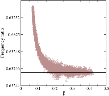
M

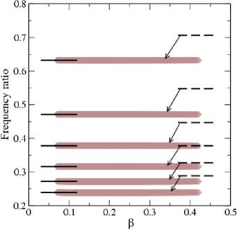
Figure 1: In the left panel we show that the ratio of the frequencies of the fundamental modes for $l=2$ and $l=3$ agrees well with that predicted by our $(l-1)(l+2)$ scaling which in this case gives a ratio of $\sqrt{5/2}\approx 0.6324555$ (shown as a solid line). The small deviation seen for low $\beta=M/R$ is typical for the first few $l$’s. The remarkable agreement for typical neutron star values $\beta\approx 0.2$ should be noted. It is also worth remarking that our numerical code has an accuracy of a few times $10^{-5}$, which means that some of the remaining spread in this range may be due to numerical error. In the right panel we show that the numerically computed ratio of the frequencies of the fundamental modes agrees well with that predicted by our $(l-1)(l+2)$ scaling (shown on the left as solid lines). The $l(l+1)$ prediction is show on the right as dashed lines. Of course, for large $l$ (so that the plane wave approximation is valid) we get $(l-1)(l+2)=l^{2}+l-2\rightarrow l(l+1)$. Nevertheless, the discrepancy for the first few values of $l$ may lead to an erroneous multipole assignation for a given observed mode-signal.

Let us now consider the various overtones $n\neq 0$ for any given $l$. We then need to solve the quadratic equation (15). Expanding the resulting square root in the small parameter $\Delta/R$ and ignoring the negative root we get

$$\omega\approx e^{\nu-\lambda}\frac{n\pi v_{r}}{\Delta}\left(1+e^{2\lambda}\frac{(l-1)(l+2)}{2\pi^{2}}\frac{v_{t}^{2}}{v_{r}^{2}}\frac{\Delta^{2}}{RR_{c}}\frac{1}{n^{2}}\right).$$ (18)

The second term in the parenthesis is negligible for moderate $l$. It is worth noting that it is $v_{t}$ that affects the $n=0$ modes whereas the $n>0$ modes are primarily determined by $v_{r}$. It should also be emphasised that condition (13) holds for the overtones, which means that our approximation is consistent in this case.

In order to estimate the overtone frequencies for any given $M$ and $R$ (say) we need to provide the crust thickness $\Delta(R,M)$ which then leads to $R_{c}$. In Appendix B we show that the crust thickness is well approximated by

$$\frac{\Delta}{R}\approx\left(\frac{\beta}{\alpha}e^{2\lambda}+1\right)^{-1},$$ (19)

where $\beta=M/R$ is the stellar compactness and $\alpha$ is a parameter that depends on the equation of state and which essentially measures some average compressibility of the crust. As discussed in Appendix B, the relevant value for our crust equation of state is $\alpha=0.02326$.

We want to combine these various approximations to get explicit expressions for the mode frequencies that can be used to compare to either numerical results for detailed relativistic models or observational data. To do this, we first assume that the crust is isotropic by setting $v_{r}=v_{t}=v$. If we then compare Eq. (16) and (18) to our full numerical results we find that they provide reasonable approximations for the same value of the shear wave speed $v$, provided that we adjust the factor of $1/2$ in (16). Since we already knew that Eq. (16) was not derived in a consistent way, this manipulation does not seem unreasonable.

The shear speed varies very little in the crust and has a value $\sim 10^{8}$ cm/s. Writing $v=v_{0}\times 10^{8}$ cm/s, where $v_{0}$ is a dimensionless parameter we may write our frequency estimates as

$$f \approx 11.85\frac{v_{0}}{R_{10}}\frac{\sqrt{(l-1)(l+2)}}{2}\sqrt{\frac{(1.705-0.705\beta_{\star})(0.1055+0.8945\beta_{\star})}{\beta_{\star}}},\quad(n=0)$$ (20)

$$f \approx 473.77n\frac{v_{0}}{R_{10}}(0.1055+0.8945\beta_{\star}),\quad(n>0)$$ (21)

where $R_{10}=R/10$ km and $\beta_{\star}=\beta/0.2068$ ($\beta_{\star}=1$ for a star with radius 10 km and mass $1.4M_{\odot}$, obtained using the most recent value for $G$ etc.). Comparing to our numerical data we find that $v_{0}\approx 2.34$. This value may appear to be surprisingly large given that, for our EOS, the maximum shear speed is about $2\times 10^{8}$ cm/s. However, it should be remembered that the parameter $v_{0}$ is obtained through comparison with the full numerical solutions and therefore represent some “weighted average” shear speed. In this (implicit) averaging geometrical factors and explicit EOS dependence may well contribute factors of order unity. In a sense, the replacement of $R$ with the geometrical mean radius of the crust $\sqrt{RRc}$ represent the first order geometrical effect. It is also worth pointing out that the simple linear scaling with $n$ does not represent the behaviour found in the numerical study. Again, this is not surprising as the eigenfunctions will have different forms and hence depend more strongly on the EOS in different parts of the crust. In general the mode frequencies seem to grow less rapidly than linear as a function of $n$. Another interesting point to note is the absence of an overall redshift factor in the estimated overtone frequencies. This somewhat counter-intuitive result arises since the redshift factor in (18) is essentially cancelled by the corresponding factor in the formula for the crust thickness.

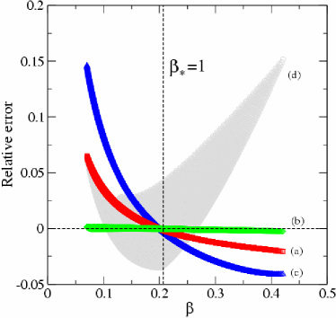
M

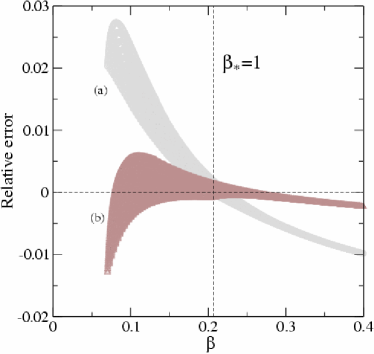
Figure 2: In the left panel we compare various estimates for the fundamental $l=2$ torsional mode. We show the relative error, compared to numerical data, of the frequency estimates as functions of $\beta$. In each case we have rescaled the estimates to give approximately the numerically computed value of the frequency at $\beta_{\star}=1$ (see the main text). This corresponds to choosing an appropriate value of the shear speed. Comparing Piro’s result (c) with ours (a) we see that the $(RR_{c})^{-1/2}$ scaling performs better than the standard $R^{-1}$. We also note that the extrapolated “general relativity correction factor” of Duncan (d) not only makes the estimate less accurate, but actually destroys the clean $\beta$-dependence. Also shown is our fit of the frequencies (b) which is accurate to within 0.2 %. In the right panel we show the relative error in the estimate for the frequency of the first overtone both with (b) and without (a) the empirical fitting factor.

The accuracy of our approximate formulae is illustrated in Figure 2. When comparing the approximations to the numerical data we note that, for the fundamental modes, the error is a smooth function of $\beta$. The situation therefore lends itself to improvement by fitting. Playing the same game with the overtones we find

$$f \approx 27.65\frac{1}{R_{10}}\frac{\sqrt{(l-1)(l+2)}}{2}\sqrt{\frac{(1.705-0.705\beta_{\star})(0.1055+0.8945\beta_{\star})}{\beta_{\star}}}\frac{\beta_{\star}}{1.0331\beta_{\star}-0.0331},\quad(n=0)$$ (22)

$$f \approx 1107.3\frac{1}{R_{10}}n(0.1055+0.8945\beta_{\star})\frac{\beta_{\star}}{1.0166\beta_{\star}-0.0166},\quad(n>0)$$ (23)

These frequency estimates are evaluated against numerical data in figure 2. We see that they perform extremely well, with relative errors typically smaller than 1%. Clearly, our various approximate formulae provide a very accurate representation of the full numerical results. We therefore anticipate that they will prove useful for any attempts to infer physical parameters from observational data.

4 Seismology

In this section we discuss how one can use our numerical and approximate results for axial modes in the neutron star crust to infer physical parameters from observations, eg. the QPOs found in the tails of magnetar flares. To carry out this analysis we assume that the observed QPOs in the frequency range $\sim 28-160$ Hz are connected with fundamental ($n=0$) elastic modes with different $l$’s, whereas the QPO at $\sim 626$ Hz is an overtone (see below for a brief summary of the observations). It is important to note that these assumptions may not be valid, especially since one can argue that the crust motion excites motion also in the core fluid via the magnetic field coupling (Glampedakis et al., 2006; Levin, 2006). If this is the case, then the mode problem that we have solved in this paper does not provide a complete picture. However, even though our analysis may not be entirely realistic in this sense we believe that our discussion provides a useful example of the strategy. We should also stress that, until fully relativistic modes for magnetised stars are calculated, this analysis may be the best one can expect.

4.1 Observations

Before considering the inverse problem of finding global neutron star properties from observed spectra let us briefly discuss the observations. So far there have been three recorded giant flares, all associated with SGRs.

SGR 0526$-$66:

This flare took place in March 5 1979 (Mazets et al., 1979). Only a weak QPO was detected at $\approx 44.5$ Hz (Barat et al., 1983). Due to the meagre data and the fact that this feature was detected in the peak of flare with significant dead-time effects in the data we will not consider this observation further.

SGR 1806$-$20:

Erupted December 27 2004 (Hurley et al., 2005; Palmer, 2005). Israel et al. (2005) detected QPOs at $18.1\pm 0.3$, $30.4\pm 0.3$ and $92.5$ Hz in the data from the Rossi X-ray Timing Explorer (RXTE). Watts & Strohmayer (2006) later examined the data from the Ramaty High Energy Solar Spectroscopic Imager (RHESSI) and found QPOs at $17.9\pm 0.1$, $25.7\pm 0.1$, $30$ (weaker), $92.7\pm 0.1$ and $626.46\pm 0.02$ Hz. Strohmayer & Watts (2006) have recently detected a feature at $\approx 150$ Hz as well as showing that the $\approx$ 30 Hz QPO is better fitted by 29 Hz. In our analysis we exclude the lower frequency QPOs. This choice is guided by our recent toy problem (Glampedakis et al., 2006). Hence, we consider the 29, 92.7, 150.3 and 626 Hz modes. The inclusion of the 150 Hz QPO does not change the conclusions substantially (which, incidentally, support the identification of the 29 Hz QPO with the $l=2$ mode and that our scaling with $l$ is the correct one). In table 1 we display these frequencies together with the modes that we identify them with.

SGR 1900+14:

A giant flare from this magnetar was detected on August 27 1998 (Hurley et al., 1999; Feroci et al., 1999). Strohmayer & Watts (2005) found evidence for QPOs at $28\pm 0.5$, $53.5\pm 0.5$, $84$, $155.1\pm 0.2$ Hz in the data from RXTE. In our analysis we use all of these frequencies. The modes that we identify them with are listed in table 1.

SGR 1806$-$20 SGR 1900+14 f [Hz] mode f [Hz] mode $29$ ${}_{0}t_{2}$ $28\pm 0.5$ ${}_{0}t_{2}$ $92.7\pm 0.1$ ${}_{0}t_{6}$ $53.5\pm 0.5$ ${}_{0}t_{4}$ $150.3$ ${}_{0}t_{10}$ $84$ ${}_{0}t_{6}$ $626.46\pm 0.02$ ${}_{1}t_{l}$ $155.1\pm 0.2$ ${}_{0}t_{11}$

Table 1: Observed QPO frequencies and suggested corresponding elastic crust modes. The identified modes are denoted according to ${}_{n}t_{l}$. Note that the true $l$-dependence differs from the standard $l(l+1)$ which explains why our identifications are different from those of Strohmayer & Watts (2005) (SGR 1900+14) and Israel et al. (2005) (SGR 1806$-$20). It may also be noted that the rather large allowed error (6 %) in our analysis makes it possible to identify the 150 Hz QPO in SGR 1806$-$20 with both an $l=9$ and and $l=10$ mode in different regions of the $M$-$R$ parameter space. However, the presence of the overtone at 626 Hz marginally rules out the $l=9$ option.

4.2 Seismology with the analytic expressions

It is straightforward to use the analytic approximations that we derived in the previous section to analyse the observed frequencies and extract the key neutron star parameters.

Let us first assume that we observe the fundamental quadrupole mode together with the first overtone $(n=1)$. In the data for SGR 1806$-$20 it seems reasonable to assume that the first is represented by the 29 Hz QPO, while the latter corresponds to the 626 Hz mode. From our approximate formulae we immediately see that the ratio of these modes provides an expression that only contains the compactness $\beta_{\star}$. In effect, the data provides a curve in the $M-R$ plane on which the true stellar model should lie. Solving this constraint for the compactness we find that $\beta\approx 0.12$, i.e. $R\approx 8.1M$. From Eq. (19) we also see that the relative crust thickness is $\Delta/R\approx 0.17$. We can then insert this value for $\beta$ in the expression for (say) the fundamental mode. This allows us to solve for the radius, and we find that $R\approx 11.4$ km, which means that $M\approx 1.41$ km $\approx 0.96M_{\odot}$ and $\Delta\approx 1.9$ km. These values do not seem unreasonable, even though the inferred mass is quite low and the crust surprisingly thick. Most likely there are systematic effects due to the magnetic field. These are, of course, not accounted for in our analysis.

Next consider the fundamental modes for different values of $l$. First note that the scaling with $l$ allows us to immediately work out the ratio of the different mode frequencies. Once we assign the $\approx$30 Hz QPO to the fundamental $l=2$ mode we can infer the multipoles of the various higher frequency modes in the observed data. The conclusions of this analysis are given in Table 1. Once we have determined the various multipoles, our approximate formula for the fundamental modes can be used to constrain the stellar parameters. Let us take the quadrupole mode as an example. If the frequency is known, then the approximate formula gives the stellar radius as a function of the compactness $\beta$. Since $M=\beta R$ we again have a constraint curve in the $M-R$ plane. In order to be consistent with the results for the $n=1$ overtone, the two curves must intersect. The point of intersection immediately provides us with the mass and radius of the star. Available results for higher $l$-modes provide further constraints that can be used to verify the consistency/accuracy of the inferred stellar parameters. Of course, since our model is an idealisation (a spherical star with an isotropic crust etcetera) one would expect the use of real data to lead to a spread of the various curves in the $M-R$ plane. This uncertainty can to some extent be used to assess the reliability of the parameter extraction.

4.3 Using numerical results to identify parameters

In our numerical code we solve the background Einstein equations together with the perturbation equations, specifying the core mass and radius. In the absence of discontinuous tangential pressure at the crust-core interface neither this boundary nor the top of the crust present any difficulties. [If there is a jump discontinuity in the tangential pressure we have one more parameter in the problem, see Karlovini & Samuelsson (2003) and Karlovini et al. (2004) for discussions.] It is therefore straightforward to integrate the equations both inwards and outwards to a matching point where we make sure that the Wronskian of the system (6) and (7) vanishes. We have checked that the results do not depend on the choice of matching pressure. The simple nature of our model allows us to quickly compute many modes ($2\leq l\leq 14$, $0\leq n\leq 3$) for a large set of core masses (45) and radii (200) numerically.

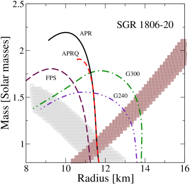
M

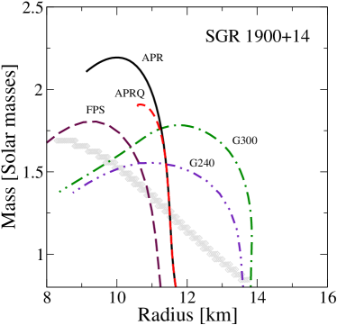
Figure 3: Seismology analysis based on our numerical axial-mode results. For the flare in SGR 1806$-$20 (left panel) we associate the lower frequency QPOs (approximately 29, 93 & 150 Hz) with fundamental ($n=0$) modes with $l=2,6,9$ or 10 respectively. The inclusion of the 150 Hz mode does not change the picture substantially. The higher frequency QPO (626 Hz) is associated with a $n=1$ mode of arbitrary $l$. The models allowed by the lower QPOs form a rather broad region that is orthogonal to the line corresponding to models that have an $n=1$ overtone of the right magnitude. As discussed in the main text, the true stellar parameters should belong to the region of overlap. For the flare in SGR 1900+14 (right panel) we use all the reported QPOs (approximately 28, 53, 84 & 155 Hz) and find that the sequence of $l$’s is (2,4,6,11). The larger number of modes leads to a narrower allowed region for the given tolerance. However, the lack of overtones in the data means that the stellar parameters are much less constrained in this case.

Our aim is to use this data set to determine models that match all the observed frequencies listed in table 1 (to some accuracy). As indicated above, one has to allow for some level of uncertainty when comparing the observed data to our numerical calculations. In our analysis we have, rather arbitrarily, chosen to allow a relative error of 6 % in the frequencies. For each of the two flares we associate a subset of the observed QPO frequencies with axial oscillation modes and search our computed data set for stellar models which has all the required frequencies, for some sequence of $l$’s. For SGR 1900+14 we use all four observed QPOs and infer that the excited modes correspond to $l=2,4,6,11$. For SGR 1806$-$20 we assume that the frequencies lower than about 30 Hz are not directly associated with axial crust oscillations [see Glampedakis et al. (2006) for a possible explanation of these modes]. We are then left with a sequence of three fundamental modes which we identify with the multipoles $l=2,6,10$. The last one, when only compared to the other fundamental modes, could also be allowed to have $l=9$ in parts of the parameter space. However, for SGR 1806$-$20 we also a higher frequency QPO which we associate with an $n=1$ overtone with arbitrary (but low) $l$. This marginally restricts the higher fundamental mode to $l=10$.

The results of the analysis are displayed in Figure 3. In each panel we plot the mass-radius relation (as lines) for a few proposed EOSs. The equations of state are chosen for illustration only and include the A18-$\delta v$+UIX^∗ model of Akmal et al. (1998) with and without a deconfined quark core (APR & APRQ), two examples from Glendenning (2000) (G240 & G300) and the FPS EOS of Pandharipande & Ravenhall (1989) (FPS). On top of this we display, as grey diamonds, the allowed masses and radii if the given set of observed low frequency QPOs are associated with elastic oscillations. In the plot of SGR 1806$-$20 the models which have an $n=1$ overtone is shown as dark squares.

The numerical results nicely illustrate the strategy for neutron star seismology discussed for the approximate formulae. In particular, the case of SGR 1806$-$20 indicates that the detection of overtone modes is extremely valuable. Given both the fundamental mode and an overtone the stellar parameters can be constrained to a relatively narrow region of the $M$-$R$ plane. This, of course, then provides useful constraints on the supranuclear core EOS.

5 Discussion

In this paper, we have considered torsional oscillation modes in neutron star crusts. Using a state-of-art EOS in the crust but otherwise simplifying the problem as far as possible we have shown how global properties of the star may be deduced from observations of such modes. We have done this using both approximate formulae and a large sample of fully numerical mode-results. As an example we applied our methods to SGRs assuming that the post-flare QPOs are connected with pure crustal oscillations. The results show that the devised strategy for asteroseismology is, in principle, quite powerful. Of course, the basic model needs to be improved before the inferred stellar parameters should be taken too seriously. In particular, we expect systematic effects due to our neglect of the magnetic field, which obviously should be important for magnetars. One can immediately think of several ways to improve upon our calculations. Below we list the most important.

For a magnetic star, one would not expect the QPOs to be exactly at the pure crustal frequencies. The toy model of Glampedakis et al. (2006) suggests that the QPOs are really global oscillations of the entire star, but that the modes that are predominately excited lie close to the pure crust modes. In addition one would expect the geometry and strength of the magnetic field to have a key role in determining which modes are excited and how strongly. Clearly, this question can only be settled in a realistic spheroidal model. Work on that problem should be strongly encouraged.

The magnetic field will not simply lead to an offset of the mode frequency with respect to that of a pure crust mode. The nature of the modes will also be affected by the presence of the field. The considerations of Piro (2005) show that (in his plane-parallel geometry) the fundamental modes are only weakly affected by the magnetic field, whereas the overtones are strongly dependent on the field. This is to be expected from our expressions (22) and (23) where we see that the fundamental modes are determined by the tangential shear velocity $v_{t}$ while the overtones instead depend on the radial velocity $v_{r}$. A magnetic field will boost the elasto-MHD speeds along the field direction and it therefore seems possible that the toroidal part of the field will affect the fundamental modes whereas the poloidal part will influence the overtones. Should this prove to be true for the spherical case it would be very interesting since it would offer a possibility of extracting information concerning the field geometry. That the geometry of the magnetic field configuration is essential to the behaviour of the torsional modes was emphasised by Messios et al. (2001) and recently by Sotani et al. (2006).

In our model we have assumed zero temperature. A non-zero temperature will lead to a systematic effect since the shear modulus will decrease (Ogata & Ichimaru, 1990). It will also mean that the crust will be slightly thinner as the ocean is deeper. In our calculations we have integrated the equations all the way to the density of iron at zero pressure.

In the deep crust matter is not expected to be microscopically isotropic, but instead form so-called pasta phases. If these anisotropies extend to macroscopic (fluid-dynamic) scales, i.e. if they do not average out over large distances compared to the lattice spacings, the radial and tangential shear speeds will be different, perhaps by a factor of two (Pethick & Potekhin, 1998). Additionally, the crust may not be in a relaxed state, causing the background strain to influence the torsional oscillations. We have not taken this into account in our model.

In the inner crust we expect that at least a portion of the dripped neutrons are in a superfluid state. It is, in fact, likely that a significant portion of the mass does not directly participate in the oscillations. Of course, the superfluid will nevertheless be set in motion via the effect of entrainment [for discussion and relevant references see Andersson & Comer (2006)]. It would be very interesting the examine the effects of this mechanism on the mode spectrum using the recently developed formalism of Carter & Samuelsson (2006) (which incidentally also allows for a MHD-type magnetic field).

Our models are static, i.e. non-rotating. Although this is a very good approximation for the slowly rotating magnetars it would be useful to extend our treatment if toroidal oscillations were to be observed in faster spinning pulsars.

Our model is non-dissipative. In reality a number of processes, including the emission of gravitational and electromagnetic radiation, will damp the oscillations. Mutual friction between superfluid and normal components in the inner crust and viscosity will also be important. Observations of the QPOs suggest a damping time of a few tens of seconds in the SGRs. It would be interesting to estimate the characteristic damping times for each damping mechanism to see if they are consistent with the observations. In addition, if the emission mechanism of the observed X-ray signal was known, a lower limit of the amplitude of the motion of the crust could be derived. This might lead to an estimate of the maximum strain in the crust and hence an assessment of the viability of elastic motion as the origin of the QPOs. Clearly, if the maximum strain exceeds the breaking strain, the oscillations cannot be of elastic origin.

Appendix A Axial perturbations in the Cowling approximation

In Newtonian theory, the so-called Cowling approximation corresponds to neglecting perturbations in the gravitational potential. The accuracy of the approximation depends on the problem under consideration. For example, while it is not a very good approximation for the fundamental $f$-mode oscillations of a fluid star it can be excellent for the class of gravity $g$-modes which are located in the surface region. Basically, the outcome depends on whether the fluid dynamics induces significant variations in the gravitational field. Another problem where the Cowling approximation is useful is that of inertial modes of rotating stars. In this case the dynamics is dominated by the Coriolis force and variations in the gravitational potential enters at higher orders in the slow-rotation expansion.

In this paper we make use of the analogous approximation in the framework of general relativity. This problem is obviously somewhat more complex owing to the fact that in general relativity the gravitational field is a dynamical entity described by a tensor field, not just a scalar potential. The relativistic Cowling approximation has a long history dating back to McDermott et al. (1983) who considered $f$, $p$ and $g$-modes in neutron stars. Their approach was to simply take the equations that had been derived by Thorne and co-workers, e.g. Thorne & Campolattaro (1967), and neglect the metric perturbations. Since the original equations are stated in a specific gauge it is not clear that this is equivalent to “throwing away the gravitational degrees of freedom”. This issue was duly noted by Finn (1988) who reconsidered the problem and suggested a different form of the approximation. However, even then the gauge problem was not considered in detail. It was later suggested by Lindblom & Splinter (1990) that the original formulation gave better results (compared to fully numerical work) than the modified version for the low order $p$-modes. One has to treat this comparison with some caution, however, because Finn’s argument is mainly relevant for the $g$-modes.

In this paper we consider torsional oscillations in the crust (as opposed to the polar perturbation case discussed above). We shall pay special attention to the gauge problem and define our approximation as neglecting the coupling between the gravitational and matter degrees of freedom rather than just setting the variations of the gravitational field to zero. It would be interesting to consider this approach also in the polar case (e.g. using the formalism of Gerlach & Sengupta (1979)) in order to compare with the work cited above.

A.1 Axial perturbations in the decoupling limit

In this appendix we make contact with recent work on relativistic elasticity theory. By default this means that we will have to be somewhat technical. However, as the complete problem formulation and all astrophysically relevant results are provided in the main text, the material provided here is only intended for readers that are interested in the technical details.

The main results (i.e. the perturbation equations) that we will describe agree with previous work in the relevant limits [see Schumaker & Thorne (1983); Yoshida & Lee (2002); Messios et al. (2001); Sotani et al. (2006)], but we extend the results in the literature to include, in principle, anisotropic and strained backgrounds. The formalism is also valid, with minor alterations, for non-static backgrounds.

We assume that the full perturbed spacetime is axisymmetric with the Killing vector generating the symmetry denoted by $\eta^{a}$ (we use lowercase Latin letters to represent spacetime indices). Since the background around which we will later linearise is assumed to be spherically symmetric this only implies trivial restrictions of generality. We write the full spacetime metric as

$$g_{ab}=\perp_{ab}+F\mu_{a}\mu_{b},\qquad\mu_{a}=F^{-1}\eta_{a},\qquad\eta^{a}\!\!\perp_{ab}=0,$$ (24)

where $F=\eta^{a}\eta_{a}=r^{2}\sin^{2}\theta$ is the norm of the Killing vector. The tensor field $\perp_{ab}$ is a metric on the manifold of Killing vector flow lines although it is generically only a metric on a submanifold of the background spacetime. Karlovini (2002) has shown that under these circumstances the axial perturbations with arbitrary matter sources are governed by the gauge invariant set of equations

$$\nabla_{b}(FQ^{ab}) =\kappa J^{a},$$ (25)

$$\nabla_{a}J^{a} =0,$$ (26)

where $\kappa=8\pi G/c^{4}$ ($=8\pi$ in geometric units) is the coupling constant in Einstein’s equations,

$$Q_{ab}=2\nabla_{[a}\delta\mu_{b]},$$ (27)

encodes the metric perturbations and

$$J^{a}=2\delta(\perp^{ab}\eta^{c}T_{bc}),$$ (28)

where $T_{bc}$ is the stress-energy tensor, describes matter perturbations. In this section the symbol $\delta$ is used to denote a perturbed quantity in an arbitrary gauge. As discussed by Karlovini (2002) the axial gauge transformations are generated by a vector field $\zeta^{a}$ given by

$$\zeta^{a}=f_{G}\eta^{a},\quad\eta^{a}\nabla_{a}f_{G}=0,$$ (29)

leading to

$$\delta\mu_{a}\rightarrow\delta\mu_{a}+\nabla_{a}f_{G}.$$ (30)

If we assume that the metric degrees of freedom are weakly coupled to matter (which should be a reasonable approximation in the relatively tenuous crust of a neutron star) we may make the approximation that $\kappa\rightarrow 0$ in the perturbation equations (we obviously still keep the gravitational constant for the background). We are then left with decoupled equations for the gravitational waves and the matter current $J^{a}$.

Note that the gauge invariant two-form $Q_{ab}$ is given solely by the geometric perturbations. Hence, to the extent that the coupling may be ignored, the gravitational-wave degrees of freedom (e.g. the $w$-modes of the star) can be described in a gauge invariant manner. We refer to equation (25) with the right hand side set to zero as the “inverse Cowling” approximation, cf. Andersson et al. (1996). In order to clarify the content of this equation, let us write it out in Regge-Wheeler coordinates. Assuming a harmonic time dependence and separating out the angular dependence in the standard manner we arrive at

$$\left(\frac{{\mathrm{d}}^{2}}{{\mathrm{d}}r_{*}^{2}}+\omega^{2}\right)Z=VZ,$$ (31)

where

$$V=2\frac{1}{r^{2}}\left(\frac{{\mathrm{d}}r}{{\mathrm{d}}r_{*}}\right)^{2}-\frac{1}{r}\frac{{\mathrm{d}}^{2}r}{{\mathrm{d}}r_{*}^{2}}+e^{2\nu}\frac{(l-1)(l+2)}{r^{2}}=\frac{e^{2\nu}}{r^{3}}\left[l(l+1)r+\frac{\kappa}{2}(\rho-p_{t})-6m(r)\right],$$ (32)

and

$$\frac{{\mathrm{d}}r}{{\mathrm{d}}r_{*}}=e^{\nu-\lambda}.$$ (33)

For matter that is unable to support strain (such as perfect fluids) this is just the standard result for axial $w$-modes (Chandrasekhar & Ferrari, 1991; Kokkotas, 1994). If, on the other hand, the matter is able to support stresses, Eq. (31) generalises the $w$-mode problem in the inverse Cowling approximation to arbitrary matter. Note that the shear modulus enters only via the necessary distinction of pressures, and hence via the background equations. Any direct appearance is removed by the inverse Cowling approximation.

The matter current $J^{a}$ on the other hand depends on the perturbed metric and is therefore not as nicely decoupled. Having defined the “gauge invariant” inverse Cowling approximation it is natural to demand that $Q_{ab}=0$ in the Cowling case. Because of (30) it is clear that this amounts to letting $\delta\mu_{a}$ be at most a gradient of a scalar (gauge) function. The matter equations will clearly depend on the type of matter. Here we will only consider conformally deforming perfectly elastic matter (Karlovini & Samuelsson, 2003; Carter & Quintana, 1972), although the generalisation to arbitrary matter is straightforward.

A.2 Elastic matter

For elastic matter the current takes the form (Karlovini & Samuelsson, 2006)

$$J^{a}=2(\rho+p_{t})FS^{ab}\nabla_{b}(\delta\tilde{\phi}-f_{G}),$$ (34)

where $p_{t}$ is the pressure in the directions tangential to the surfaces of spherical symmetry, $\delta\tilde{\phi}$ is the perturbed $\phi$-coordinate on a reference space keeping track of the relaxed matter configuration [see e.g. Karlovini & Samuelsson (2003); Carter & Quintana (1972)] and $S^{ab}$ is a metric tensor field that describes axial shear-wave propagation,

$$S^{a}{}_{b}=\mathrm{diag}(-1,v^{2}_{r},v^{2}_{t},0),$$ (35)

where $v^{2}_{r}$ and $v^{2}_{t}$ are the speed of shear waves in the radial and tangential direction, polarised in the orthogonal tangential direction, respectively. In the isotropic limit these speeds are equal and are given by

$$v^{2}=\frac{\check{\mu}}{\rho+p},$$ (36)

where $\check{\mu}$ is the shear modulus. Under a gauge transformation generated by the vector field (29) we have (Karlovini & Samuelsson, 2006)

$$\delta\tilde{\phi}\rightarrow\delta\tilde{\phi}+f_{G},$$ (37)

which means that, in any gauge, we have

$$J^{a}=2(\rho+p_{t})FS^{ab}\nabla_{b}\delta\tilde{\phi},$$ (38)

whenever $Q_{ab}=0$. Therefore (26) is also “gauge invariant”.

An intuitive approach to the relativistic Cowling approximation is to start out with the conservation equation for the stress-energy tensor and drop the perturbed metric, obtaining

$$\delta(\nabla^{a}T_{ab})=\nabla^{a}\delta T_{ab}=0.$$ (39)

From the results of Karlovini & Samuelsson (2006) it is easy to see that the axial part of the perturbed stress-energy tensor, dropping the perturbed metric, is given by

$$\delta T_{ab}=2(\rho+p_{t})\eta_{(a}S_{b)c}\nabla^{c}\delta\tilde{\phi}.$$ (40)

It is now straightforward to convince oneself that the equation resulting from (26) is identical to the projection of (39) along $\eta^{a}$. All other components vanish identically. Hence, our geometrical way of deriving the Cowling approximation agrees with the intuitive approach. The advantage we have gained is that we now have a clear picture of how gauge issues arise. Most importantly, we have qualified the approximation as neglecting the coupling between geometrical degrees of freedom and matter degrees of freedom. This strategy could prove useful in other contexts, e.g. in a derivation of the Cowling approximation for polar perturbations.

We now proceed to derive explicit equations for our elastic crust. We start by separating out the angular dependence. Assuming also a harmonic time dependence we write $\delta\tilde{\phi}=e^{i\omega t}C(\theta)F(r)$, where $C(\theta)$ turns out to be given by a Gegenbauer polynomial, see Karlovini (2002). The function $F$ has the same meaning as $Y$ in Schumaker & Thorne (1983), $T$ in Yoshida & Lee (2002), $W/r$ in McDermott et al. (1988) and $F$ of Messios et al. (2001) if the relevant limits are taken. In Schwarzschild coordinates, denoting derivatives with respect to the Schwarzschild radius $r$ by a prime, we find

$$F^{\prime\prime}+A^{\prime}F^{\prime}+BF=0,$$ (41)

where

$$e^{A} =r^{4}e^{\nu-\lambda}(\rho+p_{t})v_{r}^{2},$$ (42)

$$B =\frac{e^{2\lambda}}{v_{r}^{2}}\left[e^{-2\nu}\omega^{2}-\frac{v_{t}^{2}(l-1)(l+2)}{r^{2}}\right].$$ (43)

These equations need to be complemented by boundary conditions at the top and bottom of the crust region. These conditions are naturally taken to be that the traction $t_{a}=r^{b}\delta T_{ab}$ vanishes at the boundaries. We then have

$$t_{a}=(\rho+p_{t})\eta_{a}v_{r}^{2}r_{b}\nabla^{b}\delta\tilde{\phi}=0.$$ (44)

That the traction should vanish follows from the fact that the shear modulus, and hence the shear wave speed, is zero in the fluid or vacuum surrounding the solid. In terms of $F$ we get

$$t=r^{2}F^{\prime}=0,$$ (45)

at the boundaries. We now define a rescaled traction according to $T=e^{A}r^{-2}t=e^{A}F^{\prime}$ and use this to reduce (41) to a first order system,

$$T^{\prime} =-e^{A}BF,$$ (46)

$$F^{\prime} =e^{-A}T.$$ (47)

This system is convenient for numerical integration since there are no derivatives of the equation of state parameters such as the shear modulus and the density (which are only known in tabular form). When the background is isotropic, i.e., when the two shear-wave speeds are identical $v_{r}=v_{t}=v$, the system simplifies considerably and one obtains

$$e^{A} =r^{4}e^{\nu-\lambda}\check{\mu},$$ (48)

$$B =e^{2\lambda}\left[\frac{e^{-2\nu}\omega^{2}}{v^{2}}-\frac{(l-1)(l+2)}{r^{2}}\right].$$ (49)

The boundary conditions are now simply that $T=0$ at the top and bottom of the crust.

One can check that this system is equivalent to that obtained by Yoshida & Lee (2002), which has the correct Newtonian limit (McDermott et al., 1988). The equations of Schumaker & Thorne (1983) and Messios et al. (2001) also reduce to these equations when the metric perturbations or magnetic fields are set to zero, respectively.

Appendix B The crust thickness

In order to express the estimated crust mode frequencies in terms of just $M$ and $R$ we need to find the crust thickness as a function of these variables. To this end we approximate both the mass function and the metric function $\lambda$ as being constant and given by $e^{-2\lambda}=1-2\beta$, where $\beta=M/R$. We also use the fact that the pressure is negligible compared to $\rho$ and $\beta$ in the crust and take the equation of state to be a simple polytrope,

$$\rho=kp^{1/\Gamma},$$ (50)

with $k$ and $\Gamma$ constant. With these approximations the equation of hydrostatic equilibrium becomes

$$p^{\prime}\approx-\rho\frac{M}{r^{2}}e^{2\lambda},$$ (51)

which may be solved to yield

$$\chi p^{1/\chi}\approx ke^{2\lambda}\frac{M}{r}+\mathcal{C},$$ (52)

where $\mathcal{C}$ is an integration constant and $\chi=\Gamma/(\Gamma-1)$. Denoting the pressure at the crust-core interface (at $r=R_{c}$) by $p_{c}$ (and defining a corresponding transition density $\rho_{c}$) we solve for $\mathcal{C}$ to find

$$\mathcal{C}=\alpha-\frac{M}{R_{c}}e^{2\lambda},$$ (53)

where $\alpha=\chi p_{c}/\rho_{c}$. Putting this into (52) and setting $p(R)=0$ at the surface we obtain

$$e^{2\lambda}M\left(\frac{1}{R}-\frac{1}{R_{c}}\right)+\alpha\approx 0,$$ (54)

solving for $\Delta/R=(R-R_{c})/R$ we finally obtain

$$\frac{\Delta}{R}\approx\left(\frac{\beta}{\alpha}e^{2\lambda}+1\right)^{-1}.$$ (55)

We see that this is a function of the compactness $\beta$ only, something we have confirmed in the numerical study, see Figure 4. The value of $\alpha$ obviously depends on the equation of state. For our tabulated equation of state it can be written

$$\alpha\approx 0.0047\chi_{\mathrm{eff}},$$ (56)

where $\chi_{\mathrm{eff}}$ is an effective value. For a $\Gamma=4/3$ polytrope we obtain $\alpha\approx 0.019$. We also fitted the expression (55) using $\alpha$ as a free parameter to the numerically obtained data and found

$$\alpha\approx 0.02326,$$ (57)

agreeing well with the estimated value. This value corresponds to $\chi\approx 5$ or $\Gamma\approx\frac{5}{4}$. In our detailed numerical fits described in the main text we use (55). However, if one is satisfied with an accuracy at the 10% level then the simple approximation

$$\frac{\Delta}{R}\approx\frac{\alpha}{\beta}e^{-2\lambda},$$ (58)

is relevant for all neutron stars (since $M/R\gg 2\times 10^{-2}$).

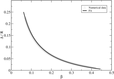
Figure 4: Fit of $\Delta/R$ with $\alpha=0.02326$ to numerical results for a large sample of stellar models. Note especially that $\Delta/R$ is (very nearly) a function of $\beta$ only, and that the simple one-parameter fit suggested by the polytropic approximation is quite accurate.

References

- Akmal et al. (1998) Akmal A., Pandharipande V. R., Ravenhall D. G., 1998, Phys. Rev. C, 58, 1804
- Andersson & Comer (2006) Andersson N., Comer G. L., 2006, ArXiv General Relativity and Quantum Cosmology e-prints (gr-qc/0605019)
- Andersson & Kokkotas (1998) Andersson N., Kokkotas K. D., 1998, Mon. Not. R. Ast. Soc., 299, 1059
- Andersson et al. (1996) Andersson N., Kokkotas K. D., Schutz B. F., 1996, Mon. Not. R. Ast. Soc., 280, 1230
- Barat et al. (1983) Barat C., Hayles R. I., Hurley K., Niel M., Vedrenne G., Desai U., Kurt V. G., Zenchenko V. M., Estulin I. V., 1983, Astron. Astrophys., 126, 400
- Carter & Quintana (1972) Carter B., Quintana H., 1972, Proc. Roy. Soc. Lond. A, 331, 57
- Carter & Samuelsson (2006) Carter B., Samuelsson L., 2006, Class. Quantum Grav., 23, 5367
- Chandrasekhar & Ferrari (1991) Chandrasekhar S., Ferrari V., 1991, Proc. Roy. Soc. Lond. A, 432, 247
- Douchin & Haensel (2001) Douchin F., Haensel P., 2001, Astron. Astrophys., 380, 151
- Duncan (1998) Duncan R. C., 1998, Astrophys. J. Lett., 498, L45
- Feroci et al. (1999) Feroci M., Frontera F., Costa E., Amati L., Tavani M., Rapisarda M., Orlandini M., 1999, Astrophys. J. Lett., 515, L9
- Finn (1988) Finn L. S., 1988, Mon. Not. R. Ast. Soc., 232, 259
- Gerlach & Sengupta (1979) Gerlach U. H., Sengupta U. K., 1979, Phys. Rev. D, 19, 2268
- Glampedakis et al. (2006) Glampedakis K., Samuelsson L., Andersson N., 2006, Mon. Not. R. Ast. Soc., 371, L74
- Glendenning (2000) Glendenning N. K., 2000, Compact Stars, second edn. Springer-Verlag, New York
- Haensel & Pichon (1994) Haensel P., Pichon B., 1994, Astron. Astrophys., 283, 313
- Hurley et al. (2005) Hurley K., Boggs S. E., Smith D. M., Duncan R. C., Lin R., Zoglauer A., Krucker S., Hurford G., Hudson H., Wigger C., Hajdas W., Thompson C., Mitrofanov I., Sanin A., Boynton W., Fellows C., von Kienlin A., Lichti G., Rau A., Cline T., 2005, Nature, 434, 1098
- Hurley et al. (1999) Hurley K., Cline T., Mazets E., Barthelmy S., Butterworth P., Marshall F., Palmer D., Aptekar R., Golenetskii S., Il’Inskii V., Frederiks D., McTiernan J., Gold R., Trombka J., 1999, Nature, 397, 41
- Israel et al. (2005) Israel G. L., Belloni T., Stella L., Rephaeli Y., Gruber D. E., Casella P., Dall’Osso S., Rea N., Persic M., Rothschild R. E., 2005, Astrophys. J. Lett., 628, L53
- Karlovini (2002) Karlovini M., 2002, Class. Quantum Grav., 19, 2125
- Karlovini & Samuelsson (2003) Karlovini M., Samuelsson L., 2003, Class. Quantum Grav., 20, 3613
- Karlovini & Samuelsson (2004) Karlovini M., Samuelsson L., 2004, Class. Quantum Grav., 21, 4531
- Karlovini & Samuelsson (2006) Karlovini M., Samuelsson L., 2006, Elastic Stars in General Relativity: IV. Axial Perturbations, preprint
- Karlovini et al. (2004) Karlovini M., Samuelsson L., Zarroug M., 2004, Class. Quantum Grav., 21, 1559
- Kokkotas (1994) Kokkotas K. D., 1994, Mon. Not. R. Ast. Soc., 268, 1015
- Levin (2006) Levin Y., 2006, Mon. Not. R. Ast. Soc., 368, L35
- Lindblom & Splinter (1990) Lindblom L., Splinter R. J., 1990, Astrophys. J., 348, 198
- Mazets et al. (1979) Mazets E. P., Golentskii S. V., Ilinskii V. N., Aptekar R. L., Guryan I. A., 1979, Nature, 282, 587
- McDermott et al. (1988) McDermott P. N., van Horn H. M., Hansen C. J., 1988, Astrophys. J., 325, 725
- McDermott et al. (1983) McDermott P. N., van Horn H. M., Scholl J. F., 1983, Astrophys. J., 268, 837
- Messios et al. (2001) Messios N., Papadopoulos D. B., Stergioulas N., 2001, Mon. Not. R. Ast. Soc., 328, 1161
- Ogata & Ichimaru (1990) Ogata S., Ichimaru S., 1990, Phys. Rev. A, 42, 4867
- Palmer (2005) Palmer D. M. e., 2005, Nature, 434, 1107
- Pandharipande & Ravenhall (1989) Pandharipande V. R., Ravenhall D. G., 1989, in Soyeur M., Flocard H., Tamain B., Porneuf M., eds, NATO ASIB Proc. 205: Nuclear Matter and Heavy Ion Collisions Hot Nuclear Matter. pp 103–+
- Pethick & Potekhin (1998) Pethick C. J., Potekhin A. Y., 1998, Physics Letters B, 427, 7
- Piro (2005) Piro A. L., 2005, Astrophys. J. Lett., 634, L153
- Samuelsson (2003) Samuelsson L., 2003, PhD thesis, Stockholm University
- Schumaker & Thorne (1983) Schumaker B. L., Thorne K. S., 1983, Mon. Not. R. Ast. Soc., 203, 457
- Sotani et al. (2006) Sotani H., Kokkotas K. D., Stergioulas N., 2006, ArXiv Astrophysics e-prints (astro-ph/0608626)
- Strohmayer & Watts (2005) Strohmayer T. E., Watts A. L., 2005, Astrophys. J. Lett., 632, L111
- Strohmayer & Watts (2006) Strohmayer T. E., Watts A. L., 2006, ArXiv Astrophysics e-prints (astro-ph/0608463)
- Thorne & Campolattaro (1967) Thorne K. S., Campolattaro A., 1967, Astrophys. J., 149, 591
- Watts & Strohmayer (2006) Watts A. L., Strohmayer T. E., 2006, Astrophys. J. Lett., 637, L117
- Yoshida & Lee (2002) Yoshida S., Lee U., 2002, Astron. Astrophys., 395, 201