Three Dimensional Compressible Hydrodynamic Simulations of Vortices in Disks

Abstract

We carry out three-dimensional, high resolution (up to $1024^{2}\times 256$) hydrodynamic simulations of the evolution of vortices in vertically unstratified Keplerian disks using the shearing sheet approximation. The transient amplification of incompressible, linear amplitude leading waves (which has been proposed as a possible route to nonlinear hydrodynamical turbulence in disks) is used as one test of our algorithms; our methods accurately capture the predicted amplification, converges at second-order, and is free from aliasing. Waves expected to reach nonlinear amplitude at peak amplification become unstable to Kelvin-Helmholtz modes when $\mid W_{\rm max}\mid\gtrsim\Omega$ (where $W_{\rm max}$ is the local maximum of vorticity and $\Omega$ the angular velocity). We study the evolution of a power-law distribution of vorticity consistent with Kolmogorov turbulence; in two-dimensions long-lived vortices emerge and decay slowly, similar to previous studies. In three-dimensions, however, vortices are unstable to bending modes, leading to rapid decay. Only vortices with a length to width ratio smaller than one survive; in three-dimensions the residual kinetic energy and shear stress is at least one order of magnitude smaller than in two-dimensions. No evidence for sustained hydrodynamical turbulence and transport is observed in three-dimensions. Instead, at late times the residual transport is determined by the amplitude of slowly decaying, large-scale vortices (with horizontal extent comparable to the scale height of the disk), with additional contributions from nearly incompressible inertial waves possible. Evaluating the role that large-scale vortices play in astrophysical accretion disks will require understanding the mechanisms that generate and destroy them.

1. INTRODUCTION

Many aspects of the structure and evolution of astrophysical accretion disks are controlled by the mechanism for angular momentum transport. When the disk is dynamically coupled to a weak magnetic field, the magnetorotational instability (MRI, e.g., Balbus & Hawley 1998) generates MHD turbulence which is a vigorous source of angular momentum transport (for a recent review, see Balbus 2003). However, in neutral or very weakly ionized disks (e.g., proto-planetary disks, and dwarf nova systems in quiescence) the magnetic field may be decoupled from the gas, and the MRI may not operate (Salmeron & Wardle 2005; Fromang, Terquem, & Balbus 2002; Gammie & Menou 1998). It these cases, it is important to investigate purely hydrodynamical mechanisms for the transport of angular momentum.

Although Keplerian shear flows are linearly stable according to the Rayleigh criterion, it has long been supposed that there exists some mechanism that produces turbulence and transport via nonlinear instabilities at high Reynolds number. To date, however, no mechanism for such instabilities has been explicitly demonstrated, and no evidence for self-sustained hydrodynamical turbulence has been found in direct numerical simulations of Keplerian disks at the same Reynolds number needed to capture known nonlinear instabilities in Cartesian shear flows (Balbus, Hawley, & Stone 1996; Hawley, Balbus & Winters 1999). Even if nonlinear instabilities exist in Keplerian shear flows, Lesur & Longaretti (2005) argue that current simulations already show the associated transport would be negligable. Recently, new interest has focused on the role that transient growth of incompressible, leading waves might play in generating hydrodynamical turbulence (Chagelishvili et al. 2003; Umurhan & Regev 2004; Yecko 2004). The amplification factor of incompressible (vortical) waves is of order $(k_{x,0}/k_{y})^{2}$, where $k_{x,0}$ and $k_{y}$ are the initial wavenumbers in the radial and azimuthal directions respectively (Johnson & Gammie 2005a, hereafter JGa). For leading waves that are initially tightly wound $\mid k_{x,0}\mid/k_{y}\gg 1$, large amplification factors are possible, potentially leading to nonlinear amplitudes. This has been suggested as one step in the route to self-sustained hydrodynamical turbulence in disks (Afshordi et al 2005; Mukhopadhyay et al. 2005; but see Balbus & Hawley 2006). One purpose of this paper is to investigate the effect of transient growth of leading waves in fully three-dimensional (3D) compressible hydrodynamical disks.

On the other hand, there is continued interest in the role that vortices play in disks. There is particular interest in the context of proto-planetary disks, where it has been suggested that vortices play a role in trapping dust and aiding in grain-growth (e.g., Barge & Sommeria 1995; Adams & Watkins 1995; Johansen, Anderson, & Brandenburg 2004). In addition, if vortices produce outward angular momentum transport they may play an important role in the structure and evolution of proto-planetary disks as well as other weakly ionized accretion disks (e.g., Li et al. 2001; Barranco & Marcus 2005, hereafter BM; Johnson & Gammie 2005b, hereafter JGb). A variety of authors have studied the evolution of random vorticity in both 2D and 3D, and in both incompressible and compressible gases. Long-lived, anticyclonic (with rotation opposite to the background shear) vortices have been found in 2D Keplerian disks (e.g., Godon & Livio 1999, 2000; Umurhan & Regev 2004; JGb). The work of JGb is particularly relevant to this study in that they considered the evolution of a spectrum of vorticity consistent with Kolmogorov turbulence in fully compressible 2D simulations. In every case, they found the kinetic energy and transport decays from the initial conditions (sustained turbulence was not evident), although the rate of decay was affected by factors such as the horizontal extent of the domain. These authors argued that compressibility significantly increases the outward angular momentum transport during the decay. Fully 3D simulations of the evolution of vorticity in stratified disks in the anelastic approximation have been presented by BM; they found vortices survive (and in fact, are produced) in the upper regions of the disk above a few scale heights. In the midplane, three-dimensional instabilities destroy vortices and reduce transport. Here we extend the work of JGb and BM by studying vortices in fully compressible unstratified disks in 3D. We will report on 3D studies of stratified disks elsewhere.

This paper is organized as follows. In Section 2 we describe the numerical methods and shearing sheet model used in our simulations. As a test, we study the evolution of both incompressible and compressible planar shearing waves in two-dimensions in section 3; we point out that at large amplitude vortical waves become Kelvin-Helmholtz unstable. In section 4 we discuss the evolution of random vortical perturbations in both 2D and 3D. We summarize and conclude in section 5.

2. METHOD

To study the local hydrodynamics of Keplerian accretion disks, the shearing sheet approximation is adopted (Hawley, Gammie, & Balbus 1995), that is the equations of motion are solved in a Cartesian frame centered at a radius $R_{0}$ in the disk, with linear extent much less than $R_{0}$, and which corotates at angular velocity $\Omega(R_{0})$ . In this frame, the Cartesian $x$ coordinate corresponds to radius and $y$ to azimuth. The hydrodynamic equations are expanded to lowest order in $H/R_{0}$ in this frame ($H\equiv c_{s}/\Omega$ is the local scale height of the disk, $c_{s}$ is the isothermal sound speed), giving

$$\frac{\partial\rho}{\partial t}+\nabla\cdot(\rho\mathbf{v})=0\ ,$$ (1)

$$\frac{\partial{\mathbf{v}}}{\partial t}+{\mathbf{v}}\cdot\nabla{\mathbf{v}}=-\frac{1}{\rho}\nabla p-2{\mathbf{\Omega}}\times{\mathbf{v}}+2q\Omega^{2}x\hat{{\mathbf{x}}}\ ,$$ (2)

$$p=c_{s}^{2}\rho\ ,$$ (3)

where $q\equiv-d\ln\Omega/d\ln R$ is the shear parameter. For Keplerian disks $q=3/2$. An isothermal equation of state is used throughout this paper. In Euler’s equation (2), the term $-2{\bf\Omega}\times{\bf v}$ is the Coriolis force in the rotating frame, and $2q\Omega^{2}x\hat{{\bf x}}$ represents the effect of tidal gravity. The latter is added as the gradient of an effective potential, which combined with the fact we use a numerical method which solves the equations in conservative form (see below), guarantees the net radial and azimuthal momentum is conserved. Vertical gravity is neglected for the unstratified disks studied here.

We have omitted an explicit viscosity in our ideal hydrodynamics formalism. We show in the next section that the numerical dissipation inherent in our scheme acts to damp short wavelength perturbations as desired (in particular, it prevents aliasing of trailing into leading waves), while having little effect on well-resolved modes (more than 16 grid points per wavelength). It is difficult to define an effective Reynolds number for our calculations, since the numerical dissipation is a steep function of resolution. We show below the amplitude errors in the evolution of shearing waves converges at better than second-order with our methods.

Our calculations begin from an equilibrium state consisting of constant density $\rho=\rho_{0}$, pressure $p=p_{0}=c_{s}^{2}\rho_{0}$, and purely azimuthal velocities corresponding to Keplerian rotation ${\bf v}={\bf v}_{0}=-q\Omega x\hat{y}$. We choose $c_{s}=\Omega=10^{-3}$ (which implies $H=1$), and $\rho_{0}=1$. Our computational domain is of size $L_{x}\times L_{y}\times L_{z}$, with $L_{x}=L_{y}=4H$ and $L_{z}=H$. In 2D runs, our domain represents the equatorial plane and is of size $L_{x}\times L_{y}=4H\times 4H$ (except in some 2D tests where $L_{x}=L_{y}=0.5H$, see §§3.2 and 3.3). Note the difference in the azimuthal velocity across the horizontal domain ($6c_{s}$) exceeds the sound speed. JGb found that in the evolution of random vortical perturbations in 2D, the amplitude and rate of decay of the resulting transport depends on the size of this velocity difference (and therefore the size of the domain). We adopt the fiducial model studied by JGb and expect, as in 2D, that the effect of compressibility will be reduced in smaller domains than studied here.

Our simulations use the 3D version of the Athena code (Gardiner & Stone 2005; 2006). Athena is a single-step, directionally unsplit Godunov scheme for hydrodynamics and MHD which uses the piecewise parabolic method (PPM) for spatial reconstruction, a variety of approximate Riemann solvers to compute the fluxes, and the corner transport upwind (CTU) unsplit integration algorithm of Colella (1990). The calculations presented here use fluxes computed using the two-shock approximation for isothermal hydrodynamics. The algorithms are second order accurate for all hydrodynamic and MHD wave families (Gardiner & Stone 2006); we demonstrate better than second-order convergence for plane waves in the shearing sheet in §3, indicating that our implementation of the shearing sheet boundary conditions in Athena is at least second-order accurate.

The computational domain is divided into a grid of $N_{x}\times N_{y}\times N_{z}$ zones. We choose $N_{x}=N_{y}\equiv N$ and $N_{z}=N/4$. We study the convergence of our numerical results using grids of size $N=32$ to $N=2048$ in two-dimensions, and $N=128$ to $N=1024$ in three-dimensions.

Important diagnostics of the flows considered here are the dimensionless angular momentum flux in fluctuations, defined as

$$\alpha\equiv\langle\rho v_{x}v_{y}^{\prime}\rangle/(\rho_{0}c_{s}^{2})\ ,$$ (4)

where $\langle\ \rangle$ denotes a volume average, and $v_{y}^{\prime}=v_{y}+q\Omega x$ is the difference in the azimuthal velocity compared to Keplerian rotation. Tests of our numerical methods using epicyclic waves show the mean radial flux $\langle\rho v_{x}\rangle$ remains zero over hundreds of shearing times, thus there is no need to correct equation (4) for any mean radial motion. The volume averaged perturbed kinetic energy density, including only motions in the horizontal plane, is

$$E_{{\rm K}}=\langle\frac{1}{2}\rho(v^{2}_{x}+v_{y}^{\prime 2})\rangle\ .$$ (5)

Finally, the $z-$component of vorticity

$$W_{z}=\frac{\partial v_{y}}{\partial x}-\frac{\partial v_{x}}{\partial y}$$ (6)

is an important diagnostic. In 2D incompressible flows, it is exactly conserved (i.e., the Lagrangian derivative $dW_{z}/dt$ is zero). In 2D, smooth, compressible flows, the potential vorticity $\tilde{W_{z}}\equiv(W_{z}+2\Omega)/\rho$ is conserved (JGa; the extra $2\Omega$ term comes from the Coriolis force in the shearing sheet formalism) if the flow is adiabatic and isentropic. However, in 2D flows with shocks both vorticity and potential vorticity can be generated through shock-curvature and shock-shock interactions (Kevlahan 1997). In 3D, $W_{z}$ can evolve freely. We track both $W_{z}$ and $\tilde{W_{z}}$ as a diagnostic of our methods, and of the effects of shocks.

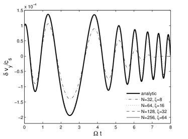
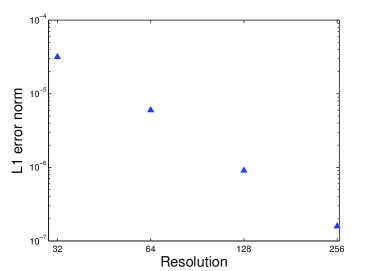
Figure 1.— Evolution of a linear amplitude, compressible, shearing wave. left: The analytic solution (heavy solid line) for the wave amplitude is compared to numerical simulations at various grid resolutions $N\times N$, where $\xi$ is the number of grid points per wavelength in the $x-$direction in the initial conditions. right: L1 error norm in the $y$-component of the velocity summed over $0\leq\Omega t\leq 6$ versus resolution. The error is converging at $N^{-2.5}$.

3. TWO-DIMENSIONAL EVOLUTION OF SHEARING WAVES

We begin by using the linear theory of plane waves in the shearing sheet as a test of our numerical algorithms. Our numerical methods then allow us to investigate what happens when leading waves are amplified to nonlinear amplitudes. We present the evolution of random vorticity fields in §4.

In the two-dimensional ($x-y$) shearing sheet, velocity perturbations representing plane waves have the form

$$v_{x}=\delta v_{x}(t)\exp[ik_{x}(t)x+ik_{y}y]\ ,\\ v_{y}+q\Omega x=\delta v_{y}(t)\exp[ik_{x}(t)x+ik_{y}y]$$ (7)

where

$$k_{x}(t)=k_{x,0}+q\Omega k_{y}t$$ (8)

and $k_{x,0}$ and $k_{y}>0$ are constant. The subscript 0 denotes quantities at the initial time $t=0$. The background shear causes the $x-$component of the wavevector to evolve linearly with time. Solutions can be divided into both compressible ($\nabla\cdot{\bf v}\neq 0$) and incompressible ($\nabla\cdot{\bf v}=0$) forms and treated analytically in the short-wavelength (i.e., $Hk_{y}\gg 1$), low-frequency ($\partial_{t}\ll c_{s}k_{y}$) limit (e.g. JGa). We consider each separately below.

3.1. Compressible plane waves

The amplitude of compressible velocity perturbations evolve according to (JGa)

$$\ddot{\delta v}_{y}+(c_{s}^{2}k^{2}+\kappa^{2})\delta v_{y}=0\ ,$$ (9)

where $\kappa^{2}\equiv 2(2-q)\Omega^{2}$ is the square of epicyclic frequency. The solution of (9) can be written in terms of parabolic cylinder functions, see JGa for details. Note that equation (9) is valid for all wavelengths and frequencies as long as the perturbed potential vorticity is zero (JGa).

Figure 1 (left) plots the evolution of a compressible shearing wave with initial wavenumbers $k_{x,0}=-4(2\pi/L_{x})$ and $k_{y}=2\pi/L_{y}$ with $L_{x}=L_{y}=4H$, and initial amplitude $\delta v_{x,0}/c_{s}=4\times 10^{-4}$. Also shown is the amplitude of the wave measured from numerical simulations at resolutions of $N=32,\ 64,\ 128,$ and 256 grid points per horizontal dimension. An important measure of the numerical resolution for plane waves is the number of grid points per initial wavelength $\lambda_{x,0}=2\pi/k_{x,0}$ in the $x-$direction,

$$\xi\equiv\frac{\mid\lambda_{x,0}\mid}{\Delta x}=\frac{2\pi N}{\mid k_{x,0}\mid L_{x}}$$ (10)

Thus, $N=32,\ 64,\ 128,$ and 256 corresponds to $\xi=8,\ 16,\ 32,$ and 64 grid points per initial wavelength respectively.

The oscillatory behavior of the amplitude of a compressible shearing wave is accurately traced by the numerical results. There is no phase error at any resolution, and at $\xi=16$ grid points per wavelength the peak amplitude of the oscillations is 0.96 of the analytic value in the first peak, and this value increases rapidly with resolution. Below this resolution the waves are smoothly damped. As a quantitative measure of the errors, figure 1 (right) plots the L1 error norm in the $y$-component of the velocity summed over the interval $0\leq\Omega t\leq 6$ as a function of numerical resolution. The slope of the line is -2.5, indicating our numerical solution is converging at better than second-order. This is direct evidence that our implementation of the shearing sheet boundary conditions, which are required to capture the evolution of shearing waves, is no less accurate than our integration algorithm.

3.2. Incompressible plane waves

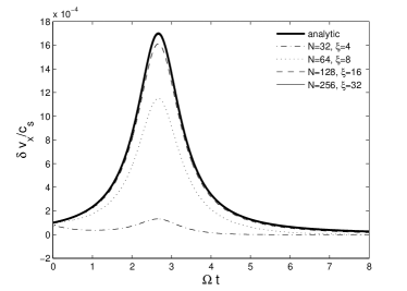
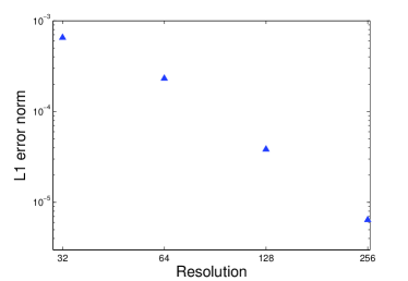
Figure 2.— Evolution of a linear amplitude, incompressible, shearing wave. left: The analytic solution (heavy solid line) for the wave amplitude is compared to numerical simulations at various grid resolutions $N\times N$, where $\xi$ is the number of grid points per wavelength in the $x-$direction in the initial conditions. right: L1 error norm in the $x$-component of the velocity summed over $0\leq\Omega t\leq 6$ versus resolution. The error is converging at $N^{-2.5}$ for $N\geq 64$.

For vortical (incompressible) shearing waves in the short-wavelength, low-frequency limit, the amplitudes of the velocity perturbation evolve as

$$\delta v_{x}=\delta v_{x,0}\frac{k_{0}^{2}}{k^{2}}\ ,\qquad\delta v_{y}=-\frac{k_{x}}{k_{y}}\delta v_{x}\ ,$$ (11)

where $k^{2}=k_{x}^{2}+k_{y}^{2}$. If the vortical wave starts as leading, i.e., $k_{x,0}<0$, it will swing to trailing at a time $t_{\rm max}=\mid k_{x,0}\mid/(q\Omega k_{y})$. During this time, the amplitude of the $x-$ component velocity perturbation is temporarily amplified, attaining a maximum value $\delta v_{x,{\rm max}}={\cal A}\delta v_{x,0}$ at $t=t_{\rm max}$, where

$${\cal A}\equiv 1+(k_{x,0}/k_{y})^{2}$$ (12)

is the peak amplification factor (e.g., Chagelishvili et al. 2003; Umurhan & Regev 2004; JGa). Note that ${\cal A}$ is also the peak amplification factor of the kinetic energy in the wave.

Figure 2 (left) plots the evolution of an incompressible shearing wave with initial wavenumbers $k_{x,0}=-8(2\pi/L_{x})$ and $k_{y}=2(2\pi/L_{y})$, and initial amplitude $\delta v_{x,0}/c_{s}=10^{-4}$. A smaller computational domain is used in this test, with $L_{x}=L_{y}=0.5H$, to minimize the effects of compressibility. To ensure the numerical representation of the perturbation satisfied the centered difference form of $\nabla\cdot{\bf v}=0$ initially, the plane wave solution is used to compute the analytic form for the $z-$component of a velocity potential $A_{z}$ which satisfies ${\bf v}=\nabla\times{\bf A}$, and then centered differences of $v_{x}=\partial A_{z}/\partial y$ and $v_{y}=-\partial A_{z}/\partial x$ are used to compute the initial velocities on the grid. Also shown is the evolution of the wave amplitude measured from numerical simulations at resolutions of $N=32,\ 64,\ 128,$ and 256 grid points per horizontal dimension, corresponding to $\xi=8,\ 16,\ 32,$ and 64 grid points per initial wavelength respectively.

The expected amplification factor for the wave is ${\cal A}=17$. As in the compressible wave case, we find our numerical solutions accurately track the analytic solution above $\xi=16$ grid points per wavelength. Below this value the wave is smoothly damped. Figure 2 (right) plots the L1 error norm in the $x$-component of the velocity summed over the interval $0\leq\Omega t\leq 6$ versus resolution; once again we find uniform convergence in the errors at a rate of 2.5 for $N\geq 64$, that is better than second-order.

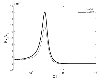
Figure 3.— Amplification of the amplitude of an incompressible plane wave at with $k_{x,0}/k_{y}=-4$ and resolutions of $64^{2}$ and $128^{2}$. Aliasing, if present, should occur at $q\Omega t=N_{x}/n_{y}-k_{x,0}/k_{y}$; note it is completely absent at both resolutions.

An important property of our numerical solutions is the lack of any aliasing. As discussed in Umurhan & Regev (2004) and JGb, aliasing is dangerous in the sense that it causes power to be artificially injected by trailing waves into leading waves, which can subsequently by amplified by the shear to repeat the loop. The symptom of aliasing is the reoccurrence of transient growth at times $\Omega t=(N_{x}/n_{y}-k_{x,0}/k_{y})/q$ (where $n_{y}=2$ is the y-direction wave number) during the decay phase of trailing waves (e.g., fig. 7 in JGb). Figure 3 shows the evolution of two runs with parameters $(k_{x,0},k_{y})=(-16\pi/L_{x},4\pi/L_{y})$, $\delta v_{x,0}/c_{s}=10^{-4}$ and N=64, 128 to $\Omega t=100$. Note that after the original peak in the amplification, the amplitude decays monotonically, without any further transient growth. We postulate that the lack of aliasing in our method is related to its dissipation properties. At low resolution (below 16 grid points per wavelength), Figure 2a shows our method smoothly damps waves. Thus, as trailing waves are sheared, our method damps them before their wavelength drops to the grid resolution and they are aliased into new leading waves. Note this does not mean our methods are overly diffusive, because the dissipation in Godunov schemes is a strong nonlinear function of resolution. Thus, for resolved waves $\xi\geq 16$ the dissipation is smaller than ZEUS-like methods. In some sense, the dissipation properties of Godunov methods are ideal for preventing aliasing.

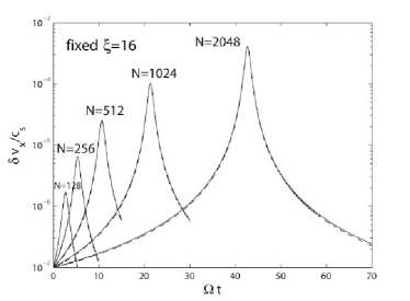
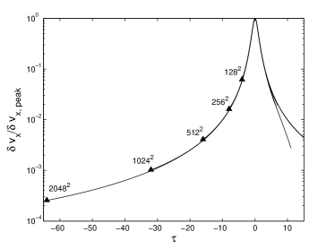
Figure 4.— Evolution of the amplitude of incompressible (vortical) plane waves with different initial $\mid k_{x,0}/k_{y}\mid$ and fixed numerical resolution $\xi=16$ grid points per wavelength. left: Curves labelled by $N=128,256,512,1024$ and $2048$ have $\mid k_{x,0}/k_{y}\mid=4,8,16,32,$ and 64 respectively. The peak amplification is ${\cal A}=17,\ 65,\ 257,\ 1025,\ 4097$. Both numerical (dashed line) and analytic (solid line) solutions are shown. right: Same as left, but plotted in terms of $\tau\equiv q\Omega t+k_{x,0}/k_{y}$.

Using fixed resolution per wavelength $\xi=16$, we have varied the initial ratio $k_{x,0}/k_{y}$ ($k_{y}=4\pi/L_{y}$ is fixed) to obtain different amplification factors ${\cal A}$. To keep the waves linear at peak amplification, we choose a very small initial amplitude $\delta v_{x,0}/c_{s}=10^{-7}$. Using grids of $N_{x}=N_{y}=128,\ 256,\ 512,\ 1024,\ 2048$, we have evolved waves with $\mid k_{x,0}/k_{y}\mid=4,\ 8,\ 16,\ 32,$ and 64 respectively, giving peak amplification factors of ${\cal A}=17,\ 65,\ 257,\ 1025$, and 4097. The results are plotted in figure 4 (left) (dashed lines) along with analytical solutions (solid lines). In each case, the numerical solution tracks the analytic accurately. As long as the initial wave is resolved, our method captures large amplification factors as well as it does small. Figure 4 (right) plots the same data, but scales the amplitude to the peak value, and uses $\tau\equiv q\Omega t+k_{x,0}/k_{y}$ as the time coordinate. The start time of each calculation is donated by a filled triangle. In this case, every curve lies atop one another, as expected.

3.3. Kelvin-Helmholtz Instability of Incompressible waves

Since with sufficient resolution it is possible to accurately follow the amplification of incompressible waves by factors of $10^{3-4}$, it is of interest to investigate what occurs when the wave reaches nonlinear amplitude ($\delta v_{x}>c_{s}$) at peak amplification. Interestingly, we have found that for some initial conditions incompressible plane wave solutions become unstable to Kelvin-Helmholtz modes quickly. Figure 5 shows the development of the KH instability in shearing wave with $k_{y}=4\pi/L_{y}$, $k_{x,0}/k_{y}=-16$, and initial amplitude $\delta v_{x,0}/c_{s}=10^{-2}$ on a $512^{2}$ grid. Four images of $\delta v_{x}$ are shown at $\Omega t=0,0.5,1.0$ and 1.5. The destruction of the plane wave is clearly evident. We have confirmed that the presence of the instability is independent of the numerical resolution. Runs on a $1024^{2}$ grid show the same behavior, although since the modes are seeded by grid noise in the initial conditions, the details change at higher resolution.

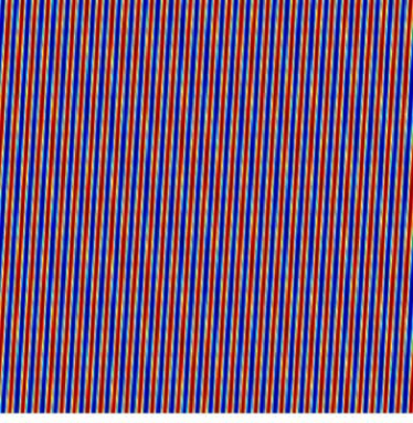
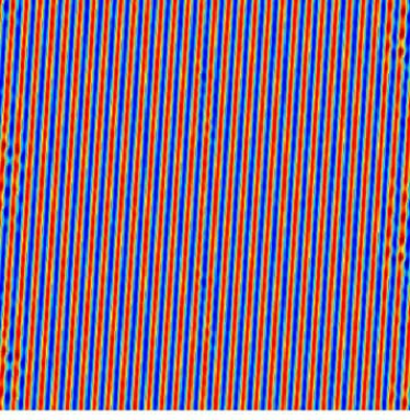
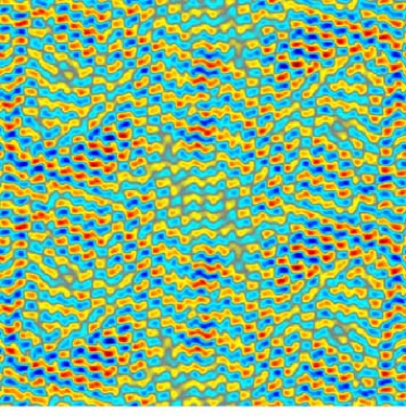
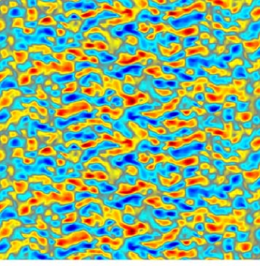
Figure 5.— KH instability in a vortical plane wave. Snapshots of the $x$-component of the velocity are shown. Parameters are $N=512$, $k_{x,0}/k_{y}=-16$, and $\delta v_{x,0}/c_{s}=10^{-2}$. Images are at intervals of $0.5\Omega^{-1}$ from the beginning of the run. The planar shearing wave is seriously distorted after only 1 shear time ($\Omega t=1$).

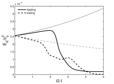
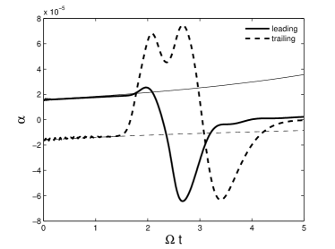
Figure 6.— Evolution of volume-averaged left: kinetic energy, and right: shear stress normalized by the gas pressure in KH unstable leading and trailing incompressible plane waves. The parameters are $\delta v_{x,0}/c_{s}=10^{-3}$, $k_{y}=4\pi/L_{y}$, $k_{x,0}/k_{y}=\mp 32$ and $N=1024$. Light curves are expected analytic solutions and heavy curves are numerical results.

Since the KH instability depends only on the amplitude of the shear but not the sign, we should expect it to affect both leading and trailing waves. By repeating the evolution shown in figure 5 but with $k_{x,0}/k_{y}=+16$, we have confirmed that even though the wave amplitude is now decaying, it is still KH unstable. In fact, the onset of the KH instability is not related to the transient amplification from leading to trailing, but is primarily determined by the initial condition. We now give some detailed analysis below.

It is instructive to use the KH instability criterion in planar flows to interpret the evolution of plane waves in the shearing sheet, even though this criterion ignores the effect of the Coriolis and tidal gravity forces. In a uniform density medium, a shear profile with an inflection point is always unstable, with a growth rate $n\sim k\delta v$. For shearing vortical waves, we might expect instability if the KH growth rate exceeds the angular velocity, that is

$$\mid k_{x}\delta v_{y}\mid\gtrsim\Omega$$ (13)

In fact, this crude criterion seems to apply remarkably well to our results. For example, simulations with $\mid k_{x,0}\mid\geq 128\pi$ and $\delta v_{x,0}=10^{-6}$ are unstable, while those with $\mid k_{x,0}\mid\leq 32\pi$ and $\delta v_{x,0}=10^{-6}$ are stable (note $k_{y}\equiv 2(2\pi/L_{y})=8\pi$ in these tests, and $\mid\delta v_{y,0}/\delta v_{x,0}\mid=\mid k_{x,0}/k_{y}\mid$). By “stable” we mean the shearing wave solution survives in both the leading phase and the trailing phase.

However, the KH instability of plane shearing waves is not related to shear amplification. Note that $\mid k_{x}\delta v_{y}\mid$ in (13) is not constant, but evolves with time. The evolution of $\mid k_{x}\delta v_{y}\mid$ can be described by (if the incompressible plane wave solution is stable):

$$\mid k_{x}\delta v_{y}\mid=\mid\delta v_{x,0}k_{y}\mid{\cal A}\bigg{[}1-\frac{1}{1+(k_{x,0}/k_{y}+q\Omega t)^{2}}\bigg{]}\ .$$ (14)

Thus $\mid k_{x}\delta v_{y}\mid$ starts from the initial value $\mid\delta v_{x,0}k_{y}\mid({\cal A}-1)$, decreases in the leading phase and becomes zero at $t_{\rm max}$; after that, it increases again in the trailing phase and approaches the limit of $\mid\delta v_{x,0}k_{y}\mid{\cal A}$. Therefore although during the shear amplification process, the perturbation amplitude $\delta v_{x}$ is amplified, the instability condition is not violated. In fact, the derivation of criterion (13) only considers azimuthal velocity shear. If one further includes radial shear, criterion (13) will be modified. The KH instability growth rate is directly related to the local maximum of vorticity (e.g., Drazin & Reid 1981), i.e., $n\sim\mid W_{\rm max}\mid\equiv\mid k_{x}\delta v_{y}-k_{y}\delta v_{x}\mid\equiv\mid\delta v_{x,0}k_{y}\mid{\cal A}$, the latter equal sign according to the analytical solution (11). Therefore criterion (13) is modified into

$$\mid W_{\rm max}\mid\equiv\mid\delta v_{x,0}k_{y}\mid{\cal A}\gtrsim\Omega\ .$$ (15)

Hence the KH instability is determined by the initial conditions. However, due to the subtlety that the shear is not steady and the position of maximum vorticity is changing, the trailing phase might have a slight preference of KH instability because $\mid k_{x}\mid$ increases during the trailing phase and the wave becomes more and more quasi-steady.

Figure 6 (left) shows the evolution of the volume averaged kinetic energy in both leading and trailing waves with parameters $\delta v_{x,0}/c_{s}=10^{-3}$, $k_{y}=4\pi/L_{y}$, $k_{x,0}/k_{y}=\mp 32$ on a $1024^{2}$ grid along with the expectation from linear theory. For the parameters adopted above, peak amplification should occur at $\Omega t=21.3$ for the trailing case. For both leading and trailing waves, the numerical solution begins to diverge significantly from the analytic curve after $\Omega t\sim 2$ of evolution. The kinetic energy rapidly decays after the KH instability saturates. The linear growth rate of the KH instability can be computed from the time evolution of the amplitude of the numerical versus analytic plane-wave solution; we measure a growth rate of about $0.2\mid W_{\rm max}\mid$, as expected for the fastest growing mode (Drazin & Reid 1981).

Figure 6 (right) shows the evolution of the volume averaged angular momentum transport $\alpha$ in both leading and trailing waves with the same parameters as in Figure 6a. The KH instability causes the value of $\alpha$ to (1) change sign, and (2) increase by a factor of about two compared to the expectation of linear theory. Note however that at late times $\alpha$ drops to near zero, that is there is no evidence for sustained transport. Thus, although it might appear attractive to suggest the KH instability is a route to turbulence and sustained transport, our simulations do not support this idea. We discuss this further in §5.

We suggest that the reason previous studies (Umurhan & Regev 2004; JGb) did not find destruction of shearing vortical waves is that they used only small initial perturbation amplitudes and intermediate amplification factors (small $\mid k_{x,0}/k_{y}\mid$), which did not satisfy the KH instability condition equation (15).

4. EVOLUTION OF VORTICES IN TWO- AND THREE-DIMENSIONS

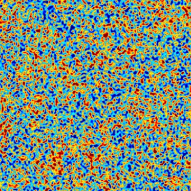
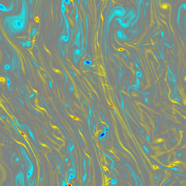
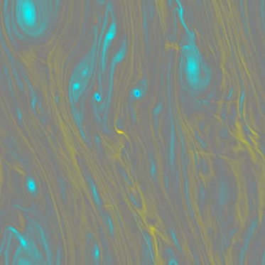
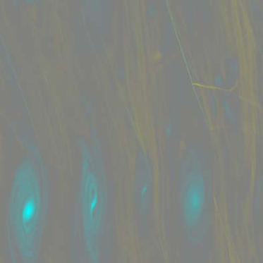
Figure 7.— Evolution of the perturbed $z$-component of vorticity $\delta W_{z}=W_{z}+q\Omega$ in 2D starting from a random distribution with a power spectrum consistent with Kolmogorov at a resolution of $1024^{2}$. The box size is $4H\times 4H$. The initial state is shown in the upper left panel. Frames are taken in lexicographic order at $\Omega t=0,\ 10,\ 20,\ 60$. Only anticyclonic vortices (blue) survive at late time.

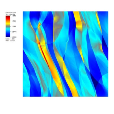
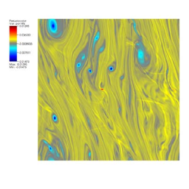
Figure 8.— Snapshots of the density (left) and potential vorticity $\tilde{W}_{z}=(W_{z}+2\Omega)/\rho$ (right) at $\Omega t=20$ in the 2D random $1024^{2}$ run.

We now consider the evolution of random vortical (incompressive) velocity perturbations in both two- and three-dimensions. Our study closely parallels the work of JGb. We draw the initial velocity perturbations from a Gaussian random field with a 2D Kolmogorov power spectrum $\mid\delta{\bf v}\mid^{2}\sim k^{-8/3}$. We apply a cut-off to the spectrum at $k_{\rm min}=\pi/H$ and $k_{\rm max}=32k_{{\rm min}}$. The amplitude of the random perturbations is characterized by $\sigma=\langle\mid\delta{\bf v}\mid^{2}\rangle^{1/2}$, we use $\sigma/c_{s}=0.8$ throughout. The effect of varying $\sigma$ was explored in JGb; smaller values lead to less angular momentum flux (see below). To ensure the perturbations are initially incompressible, we actually compute the $z-$component of a velocity potential $A_{z}$ with the appropriate power spectrum, and then compute the velocity perturbations from ${\bf v}=\nabla\times{\bf A}$. To study the effect of numerical resolution, we have found it critical to compute the power spectrum in Fourier space once and for all, and then use this same spectrum to generate the initial conditions at every resolution. This is only possible because we cut-off the power spectrum at $k=k_{\rm max}$, so there is zero power in the additional high-$k$ modes that can be represented with higher spatial resolution.

As before, the simulations all use $\rho_{0}=1$, $c_{s}=10^{-3}$, $\Omega=10^{-3}$ and a box size of $L_{x}=L_{y}=4H$ in 2D (and $L_{z}=H$ in 3D).

4.1. Random Vorticity in Two-Dimensions

We have run simulations with resolutions from $N=128$ up to $N=2048$. Figure 7 shows snapshots in the evolution of the vorticity fluctuations $\delta{W}_{z}=W_{z}+q\Omega$ for the $1024^{2}$ case. As in previous work, we confirm that cyclonic vortices (rotating in the same sense as background shear) with positive values of $\delta{W}_{z}$ are quickly destroyed, while anticyclonic vortices with negative value of $\delta{W}_{z}$ survive and decay slowly. This results in large vortices with negative $\delta{W}_{z}$ embedded in a smooth background with a slightly positive $\delta{W}_{z}$. The volume average of the vorticity fluctuations reduces to a line integral along the boundaries of our domain. Since we use periodic boundaries in $y$, this integral is a measure of the accuracy of shearing sheet boundary conditions. We find $\langle\delta{W}_{z}\rangle\sim 10^{-12}$, i.e. essentially zero, as expected.

Compressibility does play an important role in the dynamics; figure 8 is a snapshot of the density and potential vorticity $\tilde{W}_{z}$ at $\Omega t=20$ for the $N=1024$ simulation. Strong, interacting shocks which propagating primarily in the radial direction are clearly evident in the image of the density. The density contrast is more than a factor of three between the lowest and highest density regions. The locations of density jumps associated with shocks is not immediately evident in the plot of $\tilde{W}_{z}$. However, horizontal streaks of positive $\tilde{W}_{z}$ are visible, and are associated with shock intersections. As the shocks propagate over vortices, they are refracted, producing curvature in the shock front visible in the density image. At the same time, the vortices are impulsively accelerated at each shock passage. Since shocks propagate in both radial directions, vortices do not gain any net radial motion from shock accelerations, but are perturbed back and forth.

We plot the time evolution of $\alpha$ and $E_{{\rm K}}$ at each resolution in figure 9. The data points have been boxcar smoothed over an interval $\Delta t=10\Omega^{-1}$ (a smaller boxcar size $\Omega\Delta t=5$ is used for data points prior to $\Omega t=10$). Compared with fig. 4 in JGb, our $128^{2}$, $256^{2}$ and $512^{2}$ runs closely resemble their $256^{2}$, $512^{2}$ and $1024^{2}$ runs, and show some “convergence” towards higher resolution. However, our higher resolution $1024^{2}$ and $2048^{2}$ runs do not follow this trend. The time-averaged value of $\alpha$ for the last half of the runs ($100<\Omega t<200$) is of order $\sim 10^{-3}$, consistent with the highest resolution runs in JGb. Both $\alpha$ and $E_{K}$ decay by more than an order of magnitude during the evolution, and this decay shows no signs of ending. We find there can be significant differences at late times between simulations that use the same initial power-law spectra, but different initial amplitudes and phases for individual Fourier modes. We attribute this to statistical fluctuations in the small number of small $k$ modes between different realizations of the same power spectrum. The evolution of small $k$ modes depends on mode interactions at large amplitudes, and the numerical dissipation rate at linear amplitudes. Since the numerical dissipation of features resolved by 16 grid points or larger is negligible in our methods, once these small $k$ modes reach linear amplitude they decay extremely slowly, and can dominate the late-time evolution. Thus, the pattern of large-scale modes that emerges and decays at late times will depend on the initial conditions, and the history of mode interactions that occur during the evolution. Either way, because of the small number of small $k$ modes available, we expect significant statistical fluctuations between different runs at late times. Our use of boxcar averaging to smooth the data has eliminated the high-frequency fluctuations that dominate both $\alpha$ and $E_{K}$ at late times, with typical amplitudes about twice the averaged values in the plots.

The lack of convergence of $\alpha$ and $E_{{\rm K}}$ in the $1024^{2}$ and $2048^{2}$ runs bears some discussion. Note that at early times, both show the same amplitude at $\Omega t=50$, but at a much higher level than all the lower resolution runs. Thereafter, the $2048^{2}$ run decays to the same level as the other runs whereas the $1024^{2}$ run does not. This evolution seems to be related to the precise distribution of large-scale vortices that emerge in the flow. At $\Omega t=50$, images of the vorticity show four strong, well-defined vortices at the higher resolutions, whereas at lower resolution only 2-3 weaker and more diffuse vortices are evident. There are also a significant number of small, weak vortices at higher resolution. Thus, the differing rates of diffusion and merging of vortices at different resolutions may help to explain the histories.

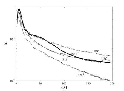
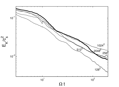
Figure 9.— Time evolution of the volume-averaged dimensionless shear stress $\alpha$ (upper) and 2-dimensional kinetic energy density (bottom) for the 2D random vorticity runs.

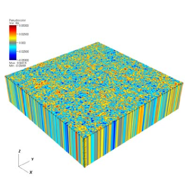
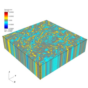
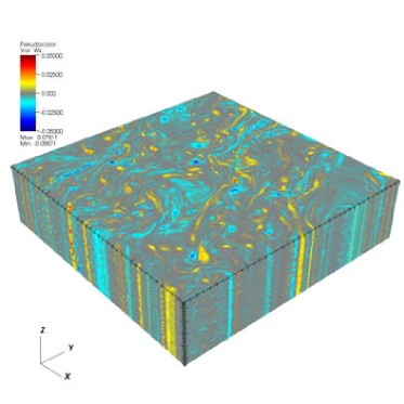
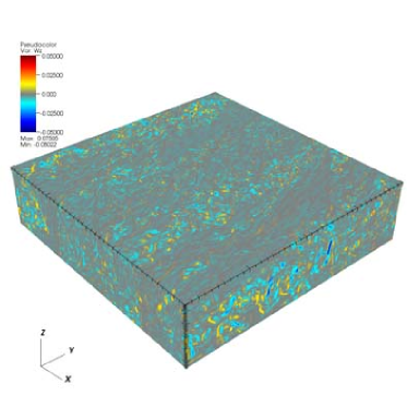
Figure 10.— Slices of the $z$ component of vorticity $W_{z}$ in the $512^{2}\times 128$ 3D random vorticity run. Snapshots are taken at $\Omega t=0,\ 10,\ 20,\ 60$.

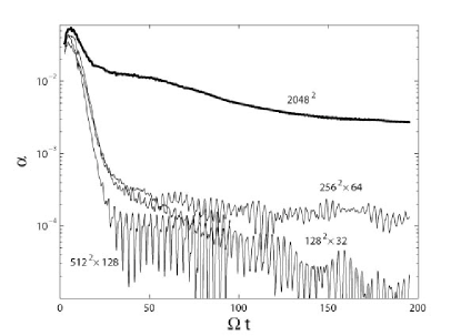
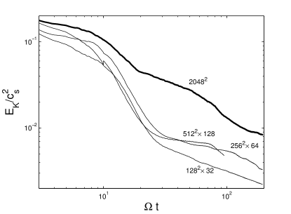
Figure 11.— Time evolution of the volume-averaged dimensionless shear stress $\alpha$ (upper) and 2-dimensional kinetic energy density (bottom) for the 3D random vorticity runs. The heavy solid curve is the result of the $2048^{2}$ 2D run for reference.

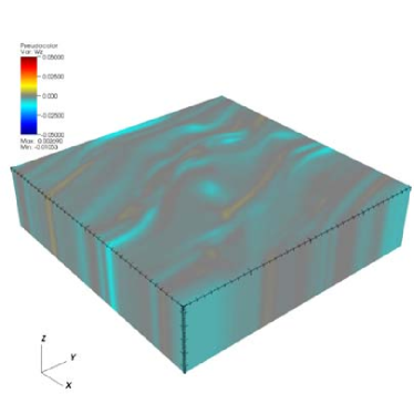
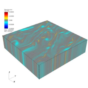
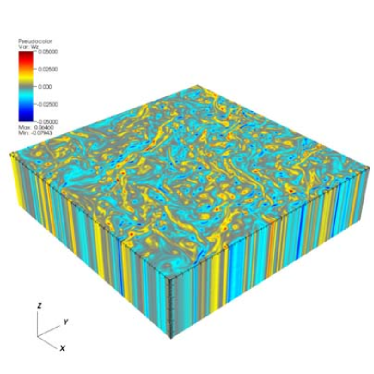
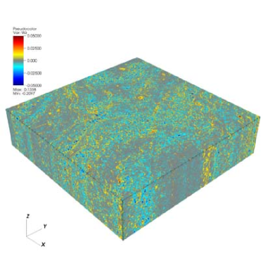
Figure 12.— Slices of the $z$ component of vorticity $W_{z}$ for the $128^{2}\times 32$, $256^{2}\times 64$, $512^{2}\times 128$ and $1024^{2}\times 256$ 3D runs taken at $\Omega t=5$.

4.2. Random Vorticity in Three-Dimensions

Using numerical resolutions of $N=128$, $256$, $512$ and $1024$, we have computed the evolution of random vortical perturbations in 3D. We use the identical initial velocity field, generated by the identical Fourier spectrum, as in the 2D case and simply project it uniformly over the third dimension. Thus, $W_{z}$ is independent of $z$ in our initial conditions, and therefore we study the evolution of vertical vortex columns in 3D. To break symmetry in the third dimension, we add small amplitude, random zone-to-zone vertical velocity perturbations with maximum amplitude $0.05c_{s}$.

Figure 10 shows snapshots in the evolution of $\delta W_{z}$ taken from the $N=512$ simulation at times of $\Omega t=0,10,20$ and 60. Note the pattern of $W_{z}$ in the x-y plane at $t=0$ is similar to the first panel of figure 7. Comparing the evolution to the 2D case, it is clear the vorticity decays much more rapidly. Vertical symmetry is maintained until $\Omega t=20$, at which point large fluctuations are present as a function of vertical position $z$. By $\Omega t=60$ the initial vortex columns have disintegrated into a complex and intertwined network of filaments that show no symmetries. The small scale structure introduced by the break up of vortex columns likely is the cause of the rapid decay. It is well known that columnar vortices are subject to elliptical instabilities (e.g., Kerswell 2002), thus the destruction of the vertical vortex tubes observed in figure 10 is not surprising. The breakdown of vortex columns has been reported in numerical simulations (e.g., BM), where the initial configurations of vortices are of known analytical forms and the growth rate can be measured for isolated vortices. Due to the complicated vortex dynamics in our simulation, i.e., background shear, vortices interacting and merging, it is difficult to quantify the destruction of vortices in terms of elliptical instability. Yet the underlying physics should be similar. The elliptical instability should exist for all two-dimensional elliptical streamlines, where 3-dimensional Kelvin-mode disturbances become unstable when resonating with the underlying strain field (e.g., Kerswell 2002). The result of the elliptical instability is to break down the vortex column into small-scale structures, which is what we find in our simulations.

Figure 11 plots the same boxcar smoothed time evolution of $\alpha$ and $E_{{\rm K}}$ from the 3D simulations, along with the $N=2048$ 2D results (heavy solid curves) for reference. The plots demonstrate how much more rapid the decay of stress and energy is in 3D compared to 2D. The evolution of stress and $E_{\rm K}$ is a rapid exponential decay (from $\Omega t\sim 10-20$) followed by a slower power-law decay. The exponential decay phase is probably associated with the breakup of the vortices and the power-law decay phase is probably associated with the decay of 3D hydro turbulence. The residual volume averaged shear stress is at least one order of magnitude smaller than that of the 2D case.

Perhaps the most striking aspect of the late time evolution of $\alpha$ and $E_{{\rm K}}$ in figure 11 are the small amplitude (linear) oscillations. By Fourier analysing the complete (rather than boxcar averaged) history of $\alpha$ and $E_{{\rm K}}$, we find a strong peak at a characteristic frequency of $0.3\Omega$. Similar, but less strong, frequency peaks are also seen at late times in the 2D runs, although at a frequency of $1.5\Omega$. This frequency depends on boxsize, a 2D box with dimensions $L_{x}=2H$ and $L_{y}=4H$ has a characteristic frequency of the late time oscillations of $0.75\Omega$. Since the oscillations are such small amplitudes, we conclude they must be related to linear modes in the shearing sheet (Balbus 2003). In 2D, only spiral density waves are possible, in 3D both acoustic and nearly incompressible inertial waves are present. The characteristic frequency expected depends on the azimuthal wavenumber $m$, as well as the ratio of the vertical to radial wavenumber for inertial waves (e.g., Balbus 2003). Since they are nearly incompressible, well-resolved (more than 16 grid points per wavelength) inertial waves should decay very slowly in our simulations. The observed frequencies are consistent with low-$m$ linear waves as the origin of the oscillations.

Figure 12 shows snapshots of $W_{z}$ at the same time $\Omega t=5$ at four different resolutions; $N=128,256,512$ and $1024$. No convergence in the spatial structure of $W_{z}$ is seen with resolution. Instead, entirely different structures are evident the same time at different resolutions. In the lowest resolution case $N=128$, the pattern of $W_{z}$ is very smooth, with the remaining fluctuations fairly symmetric in $z$. The amplitude of the fluctuations increases with resolution, with the vertical structure remaining symmetric up to the $N=512$ case. However, at $N=1024$, vertical symmetry is broken, and the vorticity has disintegrated into small scale filaments similar to those observed in the last panel of figure 10 for the $N=512$ case. The lack of convergence in $W_{z}$ is quite striking. The higher resolution simulations are able to capture higher wavenumber modes of the elliptical instabilities that lead to the destruction of vertical columns. The presence of these modes leads to destruction of the columns at an earlier time at higher resolution. This trend accounts for most of the difference in the structure between different resolutions in figure 12. The overall trend that dynamical instabilities of the vortex columns destroys the vertical symmetry and results in more rapid decay of $\alpha$ and $E_{\rm K}$ is ubiquitous at every resolution.

5. SUMMARY AND CONCLUSIONS

Using the 3D version of the Athena code (Gardiner & Stone 2005; 2006), we have carried out hydrodynamical simulations of the evolution of both planar waves and random vortical perturbations in unstratified Keplerian disks using the shearing sheet approximation. Our results can be summarized by the following four points.

(1) Our numerical methods reproduce the evolution of the amplitude of both compressible and incompressible (vortical) plane waves predicted by linear theory with negligible dissipation as long as the numerical resolution is 16 grid points per wavelength or larger. At lower resolution, the wave amplitude is smoothly damped. Significantly, there is no evidence of aliasing of trailing into leading waves as they are sheared down to the grid resolution. We have demonstrated the amplitude error in plane waves in the shearing sheet converges at better than second-order with our methods.

(2) We have shown that incompressible plane waves become KH unstable and are destroyed when $\mid W_{\rm max}\mid\gtrsim\Omega$, the condition that the growth rate of the KH instability exceeds the angular velocity. Whether the wave becomes KH unstable only depends on the initial vorticity amplitude in the initial conditions. In this case the planar shearing wave amplitude is damped well before it gets amplified by the transient growth mechanism.

(3) In 2D, the evolution of large amplitude random vorticity perturbations follows the results reported by others (Godon & Livio 1999, 2000; Umurhan & Regev 2004; JGb). In particular, coherent, large-scale (horizontal extent larger than the scale height), anticyclonic vortices survive and decay slowly. At late times the dimensionless angular momentum flux is of the order $10^{-3}$ averaged over $100<\Omega t<200$, consistent with JGb. This flux is dominated by the residual motions in the large-scale anticyclonic vortices.

(4) In 3D, the evolution of large amplitude random vorticity perturbations is similar to the 2D case, except the elliptic instabilities destroy vortex columns whose vertical extent exceeds their horizontal extent. This greatly increases the rate of decay of kinetic energy and stress. The resulting volume averaged shear stress $\alpha$ at late-times is at least one order of magnitude smaller than that for the 2D case, and is probably associated with linear amplitude, low-$m$ inertial waves that remain in the box, and which decay slowly.

The destruction of planar vortical waves by the KH instability has implications for transient amplification as a means to drive strong turbulence. Although this might appear attractive as a feedback mechanism to drive turbulence (Chagelishvili et al. 2003; Yecko 2003; Afshordi, Mukhopadhyay, & Narayan 2005), we find instability destroys the wave and results in rapid decay of kinetic energy, rather than re-seeding new leading waves. We speculate that most of the energy in the vortical wave is converted into compressible modes by the KH instability, which are not amplified by shear. Moreover, Balbus & Hawley (2006) found that these planar vortical wave solutions are actually exact to all orders and cannot serve as a route to self-sustained turbulence.

Our results show no evidence for sustained hydrodynamical turbulence in the shearing sheet. While there is non-zero transport, it is associated with large scale vortices that are introduced in the initial conditions, or which emerge from mode interactions during the nonlinear decay phase. At late times the Reynolds stress is oscillatory, which may indicate long-lived linear amplitude inertial waves also contribute to the time-averaged shear.

To understand the relevance of large-scale vortices to the dynamics of astrophysical disks, it will be important to understand how they are generated and destroyed. BM have shown that such vortices can be generated in stratified disks, but given the importance of compressible waves on the decay of vortices (JGb), it is important to investigate vortex production and evolution in fully compressible stratified disks.

References

- (1) Adams, F. C., & Watkins, R. 1995, ApJ, 451, 314
- (2) Afshordi, N., Mukhopadhyay, B., & Narayan, R. 2005, ApJ, 629, 373
- (3) Balbus, S. 2003, ARA&A, 41, 555
- (4) Balbus, S., & Hawley, J. 1991, ApJ, 376, 214
- (5) Balbus, S., & Hawley, J. 1998, Rev. Mod. Phys., 70,1
- (6) Balbus, S., & Hawley, J. 2006, ApJ, in press, astro-ph/0608429
- (7) Balbus, S. A., Hawley, J. F., & Stone, J. M. 1996, ApJ, 467, 76
- (8) Barge, P., & Sommeria, J. 1995, A& A, 195, L1
- (9) Barranco, J. A., & Marcus, P. S. 2005, ApJ, 623, 1157 (BM)
- (10) Chagelishvili, G. D., Zahn, J.-P., Tevzadze, A. G., & Lominadze, J. G. 2003, A& A, 402, 401
- (11) Colella, P. 1990, JCP, 87, 171
- (12) Drazin, P.G., & Reid, W.H., Hydrodynamic Stability, Cambridge, CUP (1981)
- (13) Fromang, S., Terquem, C., & Balbus, S.A. 2002, MNRAS, 329, 18
- (14) Gammie, C.F., & Menou. K. 1998, ApJ, 492, L75
- (15) Gardiner, T. A., & Stone, J. M. 2005, J. Comp. Phys., 205, 509
- (16) Gardiner, T. A., & Stone, J. M. 2006, J. Comp. Phys., submitted.
- (17) Godon, P., & Livio, M. 1999, ApJ, 523, 350
- (18) Godon, P., & Livio, M. 2000, ApJ, 537, 396
- (19) Hawley, J. F, Balbus, S. A., & Winters, W. F. 1999, ApJ, 518, 394
- (20) Hawley, J. F., Gammie, C. F., & Balbus, S. A. 1995, ApJ, 440, 742
- (21) Johansen, A., Anderson, A.C., & Brandenburg, A. 2004, A& A, 417, 361
- (22) Johnson, B. M., & Gammie, C. F. 2005a, ApJ, 626, 978 (JGa)
- (23) Johnson, B. M., & Gammie, C. F. 2005b, ApJ, 635, 149 (JGb)
- (24) Kevlahan, N.K.-R., 1997, J. Fluid Mech, 341, 371.
- (25) Kerswell, R. R. 2002, Annu. Rev. Fluid Mech., 34, 83
- (26) Lesur, G., & Longaretti, P.-Y. 2005, A& A, 444, 25
- (27) Li, H., Colgate, S. A., Wendroff, B., & Liska, R. 2001, ApJ, 551, 874
- (28) Mukhopadhyay, B., Afshordi, N., & Narayan, R. 2005, ApJ, 629, 383
- (29) Salmeron, R., & Wardle, M. 2005, MNRAS 361, 45
- (30) Umurhan, O. M., & Regev, O. 2004, A&A, 427, 855
- (31) Yecko, P. A. 2004, A&A, 425, 385