Primordial non-Gaussianity and Dark Energy Constraints from Cluster Surveys

Abstract

Galaxy cluster surveys will be a powerful probe of dark energy. At the same time, cluster abundance is sensitive to any non-Gaussianity of the primordial density field. It is therefore possible that non-Gaussian initial conditions might be misinterpreted as a sign of dark energy or at least degrade the expected constraints on dark energy parameters. To address this issue, we perform a likelihood analysis of an ideal cluster survey similar in size and depth to the upcoming South Pole Telescope/Dark Energy Survey (SPT-DES). We analyze a model in which the strength of the non-Gaussianity is parameterized by the constant $f\!_{N\!L}$; this model has been used extensively to derive Cosmic Microwave Background (CMB) anisotropy constraints on non-Gaussianity, allowing us to make contact with those works. We find that the constraining power of the cluster survey on dark energy observables is not significantly diminished by non-Gaussianity provided that cluster redshift information is included in the analysis. We also find that even an ideal cluster survey is unlikely to improve significantly current and future CMB constraints on non-Gaussianity. However, when all systematics are under control, it could constitute a valuable cross check to CMB observations.

1. Introduction

Of the many fascinating discoveries in cosmology over the last decade, perhaps none have aroused more interest than the discovery of the accelerated expansion of the Universe (Riess et al., 1998; Perlmutter et al., 1999). Probing the nature of the dark energy thought to be driving this acceleration has become a top priority for the community, and among the promising tools under consideration are surveys of galaxy clusters. Since the number of clusters as a function of redshift and mass depends on both the growth of structure and on the volume of space, the cluster abundance is sensitive to the matter density, the density fluctuation amplitude, and the expansion history of the Universe. For this reason, upcoming cluster surveys will be powerful probes of cosmology (e.g. Haiman et al., 2000; Holder et al., 2001; Battye & Weller, 2003; Molnar et al., 2004; Wang et al., 2004; Rapetti et al., 2005; Marian & Bernstein, 2006).

Although constraining dark energy is a leading motivator for much of the interest in cluster surveys, it is worth noting that the cluster abundance is potentially sensitive to various cosmological parameters beyond those associated with dark energy. For example, it has been recognized for some time that slight deviations from Gaussianity in the primordial matter distribution would cause a significant change in the high mass tail of the halo distribution (Lucchin & Matarrese, 1988; Colafrancesco et al., 1989; Chiu et al., 1998; Robinson et al., 1998; Robinson & Baker, 2000; Koyama et al., 1999; Robinson et al., 2000; Matarrese et al., 2000). In this paper, we use a maximum likelihood analysis to investigate the extent to which dark energy constraints from cluster surveys are degraded by including the possibility of non-Gaussian initial conditions, in particular when considered within the limits allowed by present and future CMB observations.

The specific form of non-Gaussian initial conditions we consider here is of the local type, described in position space by a primordial curvature perturbation of the form (Verde et al., 2000; Komatsu & Spergel, 2001)

$$\Phi({\bf x})=\phi({\bf x})+f\!_{N\!L}[\phi^{2}({\bf x})-\langle\phi^{2}({\bf x})\rangle]$$ (1)

where $\phi({\bf x})$ is a Gaussian random field and the degree of non-Gaussianity is parameterized in terms of the constant $f\!_{N\!L}$. For this model, tight constraints of the order of $\Delta f\!_{N\!L}\sim 40$ are provided by CMB observations (Komatsu et al., 2003; Creminelli et al., 2006; Spergel et al., 2006; Chen & Szapudi, 2006), while constraints that are somewhat weaker but that are closer in physical scale to that of clusters are expected from higher-order galaxy correlations (Scoccimarro et al., 2004). From a theoretical point of view, the non-Gaussian model of Eq. (1) is motivated in part by studies of the generation of density perturbations in inflationary scenarios; while single-field inflation models typically predict an unobservably small value for $f\!_{N\!L}$ (e.g. Acquaviva et al., 2003; Maldacena, 2003), multi-field inflation models can lead to much higher values (e.g. Lyth et al., 2003; Dvali et al., 2004; Zaldarriaga, 2004; Creminelli, 2003; Arkani-Hamed et al., 2004; Alishahiha et al., 2004; Kolb et al., 2006; Sasaki et al., 2006). For a review, see Bartolo et al. (2004).

While we believe it is worthwhile to keep an open mind to other forms of non-Gaussianity which may not be properly described by the simple expression in Eq. (1), and which might make the extrapolation of current CMB constraints to cluster scales less straightforward than we assume here (see, e.g., Mathis et al., 2004), we note that the physical scale probed by clusters differs from that of the Planck survey by roughly a factor of two, so that the two probes are likely to be affected more or less equally by deviations from Eq. (1).

As we discuss below in greater detail, the parameters in our likelihood analysis include $f\!_{N\!L}$, the matter density $\Omega_{m}$ and the matter fluctuation amplitude $\sigma_{8}$, while we consider both a constant and time-varying dark energy equations of state described in terms of one ($w$) and two ($w_{0}$ and $w_{a}$, Chevallier & Polarski, 2001; Linder, 2003) parameters respectively. For definiteness, we assume a fiducial ideal survey similar in size and depth to that of the upcoming South Pole Telescope/Dark Energy Survey (SPT-DES, Ruhl et al., 2004; Abbott et al., 2005). We assume a $\Lambda$CDM fiducial cosmology, for two values of $\sigma_{8}$, since cluster number counts are extremely sensitive to this parameter.

This paper is organized as follows. In section 2 we introduce our model for the non-Gaussian mass function and describe our analysis of the dependence of the expected errors on cosmological parameters on the non-Gaussian component. In section 3 we present our results and we conclude in section 4.

2. The model

In this section we present the methods applied in the present work. We begin with a brief review of previous works dealing with non-Gaussian initial conditions in galaxy cluster observations, and then we describe in detail our treatment of the non-Gaussian mass function. We conclude this section with a discussion of the likelihood analysis whose results will be given in section 3.

2.1. Historical overview

Expressions for the cluster mass function in the presence of non-Gaussian initial conditions have been derived as extensions to the Press-Schechter ansantz (PS, Press & Schechter, 1974) first by Lucchin & Matarrese (1988) and Colafrancesco et al. (1989) while a simpler approach has been adopted later by Chiu et al. (1998) and Robinson et al. (1998).

The original PS formula describes the comoving number density $n(M)dM$ of clusters with mass in the interval $(M,M+dM)$ as

$$n_{PS}(M)dM=-\frac{2\bar{\rho}}{M}\frac{d}{dM}\left[\int_{\delta_{c}/\sigma_{M}}^{\infty}P_{G}(y)dy\right]dM,$$ (2)

where we suppress, for clarity, the redshift dependence, $\bar{\rho}$ is the comoving mass density, $\sigma_{M}$ is the r.m.s. of mass fluctuations in spheres of radius $R=(3M/4\pi\bar{\rho})^{1/3}$, $\delta_{c}=1.686$ is the critical linear overdensity in the spherical collapse model and $P_{G}$ is the Gaussian probability distribution function (PDF), $P_{G}(y)=e^{-y^{2}/2}/\sqrt{2\pi}$. Since the function $P_{G}(y)$ does not depend explicitly on the mass $M$, and therefore on the scale $R$, Eq. (2) reduces to

$$n_{PS}(M)dM=-\frac{2\bar{\rho}}{M^{2}}\frac{\delta_{c}}{\sigma_{M}}\frac{d\ln\sigma_{M}}{d\ln M}P_{G}(\delta_{c}/\sigma_{M})dM.$$ (3)

The PS formalism assumes that the scale dependence of the PDF of the density field is completely described by the scale dependence of the variance $\sigma_{M}^{2}$. Lucchin & Matarrese (1988), Colafrancesco et al. (1989) and, later Matarrese et al. (2000) considered a derivation of the non-Gaussian mass function, based on Eq. (2), that takes into account the scale dependence of higher order cumulants, thereby allowing for a generic dependence of the PDF on the smoothing scale $R$. Specifically, Matarrese et al. (2000) (hereafter MVJ) derived the mass function corresponding to the model described by Eq. (1). The non-Gaussianity of the mass function is described, in first approximation, in terms of the skewness $S_{3,R}$ of the smoothed density field $\delta_{R}$,

$$S_{3,R}\equiv\frac{\langle\delta_{R}^{3}\rangle}{\langle\delta_{R}^{2}\rangle^{2}},$$ (4)

and it is obtained from the cumulant generator of the distribution as

$$n_{MVJ}(M)dM\simeq-\frac{2\bar{\rho}}{M^{2}}\frac{1}{\sigma_{M}}\times\qquad$$

$$\times\left[\frac{1}{2}\frac{\delta_{c}^{3}}{\delta_{*}}\frac{dS_{3,R}}{d\ln M}+\delta_{*}\frac{d\ln\sigma_{M}}{d\ln M}\right]\frac{e^{-\delta_{*}^{2}/(2\sigma_{M}^{2})}}{\sqrt{2\pi}}dM,$$ (5)

where $\delta_{*}=\delta_{c}\sqrt{1-S_{3,R}\delta_{c}/3}$.

It’s worth noticing here that although Eq. (1) should be seen as a truncated expansion in powers of $\phi$, the mass function provided by Eq. (2.1) is not linear in the non-Gaussian parameter $f\!_{N\!L}$ (since $S_{3,R}\sim f\!_{N\!L}$); rather it describes the non-Gaussian PDF by its proper dependence on the skewness while neglecting all higher order cumulants.

The simpler extension to non-Gaussian initial conditions introduced by Chiu et al. (1998) consists instead of replacing the Gaussian function $P_{G}(y)$ in Eq. (3) by the appropriate, non-Gaussian PDF $P_{NG}(y)$, assumed to be scale-independent. The resulting mass function, which we will denote here as “extended-PS” or EPS, therefore reads

$$n_{EPS}(M)dM=-\frac{2\bar{\rho}}{M^{2}}\frac{\delta_{c}}{\sigma_{M}}\times$$

$$\times\frac{d\ln\sigma_{M}}{d\ln M}P_{NG}(\delta_{c}/\sigma_{M})dM.$$ (6)

This approach, has been tested in N-body simulations by Robinson & Baker (2000) for several non-Gaussian models; they find that Eq. (2.1) agrees with measurement of the cumulative mass function $n(>M)$ in the simulations to within $25\%$. While this error is slightly larger than the differences between the PS formula, Eq. (2), and simulation results for Gaussian initial conditions, it is much smaller than the model-to-model differences between the cumulative mass functions. As a measure of the non-Gaussianity of the tail of the distribution function $P_{NG}(y)$, Robinson et al. (1998) introduced the parameter $G$ (there called $T$) defined as

$$G=\frac{\int_{3}^{\infty}P_{NG}(y)dy}{\int_{3}^{\infty}P_{G}(y)dy}$$ (7)

with $G=1$ corresponding to the Gaussian case.

Following this approach Robinson et al. (1998), Koyama et al. (1999) and Willick (2000) placed constraints on primordial non-Gaussianity from X-ray cluster survey observations (Henry & Arnaud, 1991; Ebeling et al., 1996; Henry, 1997) and Amara & Refregier (2004) relate primordial non-Gaussianity with the normalization of the dark matter power spectrum. In particular, assuming that the non-Gaussian primordial field can be generically described by a log-normal distribution, Robinson et al. (2000) found, for a $\Lambda$CDM cosmology, the constraint $G<6$ at $2\sigma$ level. An analysis of the constraining power of future Sunyaev-Zel’dovich (SZ) cluster surveys on cosmological parameters which includes the possibility of primordial non-Gaussianity is provided by Benson et al. (2002). Specifically, this work assumes the log-normal PDF studied by Robinson et al. (2000) and performs a Fisher-matrix analysis that includes the matter and baryon density parameters $\Omega_{m}$ and $\Omega_{b}$, $\sigma_{8}$ and the non-Gaussian factor $G$. The results for the 1-$\sigma$ errors on $G$, assuming priors from CMB, Large-Scale Structure (LSS) and supernovae (SN) observations, are $\Delta G\simeq 2$ and $\Delta G\simeq 0.1$ for the Bolocam and Planck experiments respectively.

Finally, Sadeh et al. (2006) apply the same extended PS formalism to the $\chi_{m}^{2}$ non-Gaussian model (White, 1999; Koyama et al., 1999). Here, however, much attention is devoted to highly non-Gaussian models, e.g., with $m=1$ and $2$, which are already excluded by measurements of the galaxy bispectrum in the PSCz survey (Feldman et al., 2001).

2.2. The non-Gaussian mass function

In our analysis we will make use of the EPS approach, Eq. (2.1), since it can be more easily implemented (once the probability function $P_{NG}(y)$ is known) and avoids problems with small regions of the parameter space where the MVJ expression for the mass function, Eq. (2.1), is beyond its limits of validity. For most of the cases considered in section 3, however, we performed the analysis using both approaches, finding almost identical results.

Since the PS and EPS expressions are known to differ by up to $25\%$ from N-body results, we use the EPS non-Gaussian mass function only to model departures from the Gaussian case; for the latter we use an analytic mass function fit to the N-body results. Specifically, we consider the non-Gaussian mass function $n(z,M,f\!_{N\!L})$ to be given by the product

$$n(z,M,f\!_{N\!L})=n_{G}(z,M)\;F_{NG}(z,M,f\!_{N\!L}),$$ (8)

where $n_{G}(z,M)$, corresponding to the Gaussian case, is the fit to N-body simulations provided by Jenkins et al. (2001),

$$n_{G}(z,M)dM=-0.301\frac{\rho_{m}}{M\sigma_{M}}\frac{d\sigma_{M}}{dM}\times$$

$$\exp\left[-|0.64-\log[D(z)\sigma_{M}]|^{3.82}\right],$$ (9)

where $D(z)$ is the linear growth factor computed by solving the differential equation governing structure evolution. The non-Gaussian factor $F_{NG}(z,M,f\!_{N\!L})$ is derived from the EPS mass function and simply given by

$$F_{NG}(z,M,f\!_{N\!L})\equiv\frac{n_{EPS}(z,M,f\!_{N\!L})}{n_{PS}(z,M)}$$ (10)

where $n_{PS}$ is the Gaussian PS mass function. Note that for $f\!_{N\!L}=0$ we have $n_{EPS}=n_{PS}$.

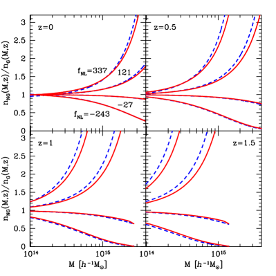
Figure 1.— Uncertainty on the mass function $n(M,z)$ due to non-Gaussianity expressed as the ratio between the non-Gaussian to the Gaussian mass function at four different redshifts ($0$, $0.5$, $1$ and $1.5$) for different values of $f\!_{N\!L}$. The inner continuous lines corresponds to the (2-$\sigma$) limits $-27<f\!_{N\!L}<121$ derived from the WMAP (first year) constraints on $f\!_{N\!L}$ by Creminelli et al. (2006) while the outer continuous lines corresponds to the limits $-243<f\!_{N\!L}<337$ from the expected SDSS galaxy bispectrum constraints (Scoccimarro et al., 2004) computed with the EPS approach, Eq. (2.1). The dashed lines, almost coincident with the continuous ones, correspond to the same limits computed by means of the MVJ formula, Eq. (2.1).

It can be easily shown that the predictions of the EPS and MVJ methods are very close by comparing them for relevant values of the parameter $f\!_{N\!L}$. In Fig. 1 we plot the ratio of the non-Gaussian mass function to the Gaussian one at different redshifts and as a function of the mass $M$ for the 2-$\sigma$ limits

$$-27<f\!_{N\!L}<121,$$

obtained from the bispectrum analysis of the WMAP 1-year data by Creminelli et al. (2006), yielding constraints that are slightly tighther than but consistent with those obtained from the WMAP 3-year data by Spergel et al. (2006). We plot as well the limits

$$-243<f\!_{N\!L}<337,$$

corresponding to the 1-$\sigma$ error $\Delta f\!_{N\!L}=145$ expected from measurements of the galaxy bispectrum in the Sloan Digital Sky Survey (SDSS) main sample (Scoccimarro et al., 2004). Notice that in the latter case we are assuming here as fiducial value for the non-Gaussian parameter $f\!_{N\!L}=47$, i.e. the maximum likelihood value of the cited WMAP analysis. The continuous lines denote therefore the allowed region computed by means of the EPS formula, Eq. (2.1), while the dashed lines corresponds to the same quantity determined assuming the EPS formalism of Eq. (2.1).

The non-Gaussian PDF $P_{NG}(y)$ that appears in the EPS formula, Eq. (2.1), is measured from realizations on a $512^{3}$ grid in a box of $1\,h^{-1}\,{\rm Gpc}$ side of the curvature perturbation $\Phi$ described by Eq. (1) in terms of the Gaussian field $\phi$, generated in Fourier space with a scale invariant power spectrum. The field $\Phi$ is then converted into the mass density field in Fourier space by means of Poisson equation and a transfer function computed by the CMBFAST code (Seljak & Zaldarriaga, 1996), smoothed on a $R=4\,h^{-1}\,{\rm Mpc}$ scale and the probability distribution is finally measured in position space. We determine a probability function for a set of values of $f\!_{N\!L}$ from $-500$ to $500$ and then interpolated to the desired value. We assume, in all cases, the fiducial cosmology described below. In order to reliably estimate the tail of the distribution, several thousands realizations were needed for each value of $f\!_{N\!L}$. For high values of the mass $M$ and redshift, corresponding to extremely rare events (7-$\sigma$), the probability distributions could not be properly determined, as can be seen from the limited plots in the lower panels in Fig. 1. None of the results in the paper, however, is sensitive to this cut-off.

It is evident from the figure that the difference between the two approaches, for this non-Gaussian model, is small, essentially noticeable just for large values of $f\!_{N\!L}$. This is due to the relatively mild dependence on the smoothing scale $R$ of the reduced skewness $s_{3,R}\equiv S_{3,R}\sigma_{R}$ for our non-Gaussian model, as we tested as well by choosing different smoothing lengths for the probability distributions measured from the realizations. On the other hand, the close results obtained by the different methods show how the degree of non-Gaussianity currently allowed can be described by the first moments of the primordial distribution, if not by the skewness alone. It is worth stressing, however, that both prescriptions for the non-Gaussian mass function, even when limited to modeling deviations from the Gaussian case, need to be properly tested against N-body simulations. New results in this direction will soon be available (Matarrese, 2006).

By means of the mentioned measured probability functions, in the framework of the EPS approach, it is also possible to translate the constraints on the parameter $f\!_{N\!L}$ into constraints on the parameter $G$ defined in Eq. (7). As an example, the WMAP 1-$\sigma$ error $\Delta f\!_{N\!L}=37$ (Creminelli et al., 2006) corresponds to $\Delta G\simeq 0.06$ while the expected 1-$\sigma$ error $\Delta f\!_{N\!L}=145$ from SDSS galaxy bispectrum measurement corresponds to $\Delta G\simeq 0.25$.

2.3. Likelihood analysis

In this section we describe the likelihood analysis we use to obtain our results. We will consider two simple models depending on four and five parameters. In addition to $f\!_{N\!L}$ we consider the matter density parameter $\Omega_{m}$, fluctuation amplitude parameter $\sigma_{8}$ and we will separately consider the cases of dark energy with either a constant equation of state parameter ($w$) or a time-varying equation of state described by two parameters ($w_{0}$ and $w_{a}$). In all cases we assume a spatially flat cosmological model for simplicity.

The fiducial values assumed for the likelihood analysis are given in Table 1. Since the expected number of observable clusters is highly dependent on the value of $\sigma_{8}$, for the four parameter model we perform the analysis assuming as well the lower value $\sigma_{8}=0.75$, while in every other case we assume $\sigma_{8}=0.9$. The choice of the fiducial value $f\!_{N\!L}=47$ for the non-Gaussian parameter does not substantially affect any of the results of the present work.

Unless otherwise stated, we consider an ideal survey with limiting mass $M_{lim}=1.75\times 10^{14}\,h^{-1}\,{\rm M}_{\odot}$ and with a sky coverage of $4000$ deg² ($f_{sky}\simeq 10\%$) out to a maximum cluster redshift of $1.5$, corresponding to the expectations for the SPT and DES projects. For our fiducial model with $\sigma_{8}=0.9$ and $f\!_{N\!L}=47$, this yields a total of $21,000$ clusters in $15$ redshift bins; if we had instead chosen $f\!_{N\!L}=0$ for the fiducial model, we would obtain $20,000$ clusters, consistent with earlier estimates (Wang et al., 2004).

We study the dependence on cosmology and on the constant $f\!_{N\!L}$ of the total number and mass distribution of clusters above a certain fixed, i.e. redshift independent, threshold mass $M_{lim}$ and explore the degeneracies introduced by varying non-Gaussian initial conditions. While the redshift dependence of the threshold mass should be included when making precise predictions for a given survey, this dependence is weak for SZ-selected cluster samples; as a result, our neglect of such dependence here will not significantly affect our conclusions.

Table 1 Fiducial values for the cosmological and non-Gaussian parameters.

Parameter		Fiducial value
$\Omega_{m}$	matter density	$0.27$
$\sigma_{8}$	galaxy fluctuation amplitude	$0.9$ ($0.75$)
$w$/$w_{0}$	dark energy equation of state	$-1$
$w_{a}$	dark energy equation of state	$0$
$f\!_{N\!L}$	non-Gaussian parameter	$47$
$n_{s}$	scalar spectral index	$1$
$h$	Hubble parameter	$0.72$
$\Omega_{b}h^{2}$	physical baryon density	$0.0232$
$\Omega_{\Lambda}$	dark energy density	$1-\Omega_{m}$

The total number of clusters with mass $M$ above $M_{lim}$, per unit redshift, is given by

$$\frac{dN}{dz}=\Delta\Omega\frac{dV}{dzd\Omega}(z)\int_{M_{lim}}^{\infty}n(z,M,f\!_{N\!L})dM$$ (11)

where

$$\frac{dV}{dzd\Omega}(z)=\frac{1}{H(z)}\left[\int_{0}^{z}\frac{dz^{\prime}}{H(z^{\prime})}\right]^{2}$$ (12)

is the cosmology-dependent volume factor for flat models and $\Delta\Omega$ is the solid angle subtended by the survey area.

We show in Fig. 2 the sensitivity of the total number of clusters above $M_{lim}$ per unit redshift and unit area (upper panels) and of the comoving number density (lower panels) to different values of the non-Gaussian parameter $f\!_{N\!L}$ compared with the sensitivity to different values of the dark energy equation of state parameter $w_{0}$ and of the fluctuation amplitude parameter $\sigma_{8}$.

Fig. 2 (upper left panel) shows that varying $f\!_{N\!L}$ over the range allowed by current CMB observations yields changes in the cluster counts comparable to a $10\%$ variation in the dark energy equation of state parameter $w$. However, the upper right panel of Fig. 2 shows that the redshift dependence of the mass function variations due to non-Gaussianity are different from the variations due to changes in $w$. This is essentially due to the fact that $w$ affects both the mass function and the volume factor. On the other hand, the redshift dependence of variations due to changes in $f\!_{N\!L}$ appears more similar to variations induced by changes in $\sigma_{8}$, so we expect a stronger degeneracy between these two parameters.

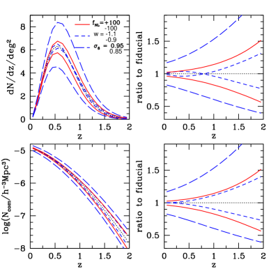
Figure 2.— Cluster counts per unit redshift (upper panels) and comoving cluster density (lower panels) as a function of redshift for different values of the non-Gaussian parameter $f\!_{N\!L}$ ($f\!_{N\!L}=\mp 100$, continuous lines), of the dark energy equation of state parameter $w$ ($w=-1.1$ and $-0.9$, short-dashed lines) and of $\sigma_{8}$ ($\sigma_{8}=0.85$ and $0.95$, long-dashed lines) compared to the fiducial case (dotted line) with $\sigma_{8}=0.9$, $w=-1$ and $f\!_{N\!L}=0$. Assumes the mass limit $M_{lim}=1.75\times 10^{14}\,h^{-1}\,{\rm M}_{\odot}$.

In Fig. 3 we show the sensitivity of the mass function $n(M,z)$ on the same parameters, this time as a function of the mass $M$ for $z=0$ (upper panels) and $z=1$ (lower panels). In this case the behavior of the cluster density as we vary $f\!_{N\!L}$ and $\sigma_{8}$ is quite different. One can clearly see how non-Gaussianity is particularly significant for the high-mass tail of the distribution. This fact suggests that it might be relevant to consider a likelihood analysis that takes into account the full functional shape of the mass function by dividing the observable clusters in mass bins (see, for instance, Hu, 2003; Lima & Hu, 2005; Marian & Bernstein, 2006). In this way one might expect to mitigate the $f\!_{N\!L}$-$\sigma_{8}$ degeneracy evident from Fig. 2 and better study the possibility of constraining non-Gaussianity with cluster surveys.

In the next section we will consider the two cases of an analysis involving a single mass bin defined by $M>M_{lim}$ and of an analysis with several mass bins. The likelihood function is based on the assumption of Poisson statistics for the cluster number measurements in each redshift bin, so that, for the single mass bin case we have

$$\ln{\mathcal{L}}=\sum_{i=1}^{N_{tot}^{z}}\left[N_{i}\ln N_{i}^{*}-N_{i}^{*}-N_{i}\ln N_{i}+N_{i}\right]$$ (13)

where $N_{tot}^{z}$ is the total number of redshift bins, $N_{i}^{*}$ is the fiducial number count in the $i$-th redshift bin, $N_{i}$ is the number count of clusters in the $i$-th redshift bin for the specific model. Throughout the paper, we consider $N_{tot}^{z}=15$ redshift bins with width $\Delta z=0.1$ out to $z=1.5$.

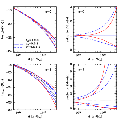
Figure 3.— The mass function $n(M,z)$ as a function of the mass $M$ at $z=0$ (upper panels) and $z=1$ (lower panels) for different values of the non-Gaussian parameter $f\!_{N\!L}$ (continuous lines), of the dark energy equation of state parameter $w_{0}$ (short-dashed lines) and of $\sigma_{8}$ (long-dashed lines) compared to the fiducial case (dotted line) with $\sigma_{8}=0.9$, $w=-1$ and $f\!_{N\!L}=0$.

In the case of multiple mass bins, the likelihood function is of the form

$$\ln{\mathcal{L}}=\sum_{i=1}^{N_{tot}^{z}}\sum_{j=1}^{N_{tot}^{M}}\left[N_{ij}\ln N_{ij}^{*}-N_{ij}^{*}\right.$$

$$\left.-N_{ij}\ln N_{ij}+N_{ij}\right]$$ (14)

with $N_{tot}^{M}=10$ being the total number of mass bins logarithmically spaced from $M_{lim}$ to $M_{\rm max}=5\times 10^{15}\,h^{-1}\,{\rm M}_{\odot}$; here $N_{ij}$ is the number of model clusters in the $i$-th redshift bin and $j$-th mass bin.

The marginalization of the likelihood functions is performed on a regular grid with a varying number of points chosen to optimize the sampling of the parameter space.

We do not include systematic errors which a real survey will encounter, including uncertainties in the cluster mass-observable relation (e.g. Seljak, 2002; Levine et al., 2002; Pierpaoli et al., 2003; Majumdar & Mohr, 2003, 2004; Hu, 2003; Lima & Hu, 2004; Francis et al., 2005; Lima & Hu, 2005; Kravtsov et al., 2006) and in cluster redshift determination (e.g. Huterer et al., 2004). We excluded as well statistical uncertainties related to sample variance (e.g. Hu & Kravtsov, 2003) or theoretical uncertainties in the cluster mass function and its cosmological dependence (e.g. Heitmann et al., 2005; Warren et al., 2006; Reed et al., 2006; Crocce et al., 2006). Finally, we note that other degeneracies with parameters such as those describing spatial curvature (Abbott et al., 2005) and the effect of massive neutrinos on the dark matter power spectrum (Huterer & Linder, 2006) might be relevant for future high precision analyses.

3. Results

In this section we estimate the impact of marginalizing over the non-Gaussian parameter $f\!_{N\!L}$ on the determination of the dark energy equation of state as well as on two other relevant cosmological parameters such as the matter density $\Omega_{m}$ and fluctuation amplitude $\sigma_{8}$. We will separately consider the case of a dark energy equation of state determined by a single parameter ($w$) and the case of a two-parameter description of a time-varying equation of state ($w_{0}$ and $w_{a}$).

We derive the marginalized errors on the parameters with fixed $f\!_{N\!L}=47$ (no marginalization) and with three different Gaussian priors on $f\!_{N\!L}$, two corresponding to the constraints from CMB bispectrum measurements expected from the Planck experiment (Komatsu & Spergel, 2001; Liguori et al., 2006) and measured in the WMAP experiment (Creminelli et al., 2006) with

$$f\!_{N\!L}=47\pm 5\qquad({\rm 1-}\sigma,~{}{\rm Planck})$$ (15)

and

$$f\!_{N\!L}=47\pm 37\qquad({\rm 1-}\sigma,~{}{\rm WMAP}),$$ (16)

and a third corresponding to the expected constraints from the analysis of the SDSS main sample galaxy bispectrum (Scoccimarro et al., 2004),

$$f\!_{N\!L}=47\pm 145\qquad({\rm 1-}\sigma,~{}{\rm SDSS~{}forecast}).$$ (17)

This last case is motivated by a possible strong scale-dependence of primordial non-Gaussianity, not captured by the model defined by Eq. (1), that could result in a stronger non-Gaussian effect at smaller scales, thereby escaping the CMB constraints. As a rough estimate of the smallest scale probed by the mentioned experiments, we notice that for WMAP, the maximum multipole $l_{max}\simeq 1000$ corresponds to $\sim 50\,h^{-1}\,{\rm Mpc}$ while Planck is expected to probe a scale three times smaller; in the SDSS case a maximum comoving wavenumber $k_{max}\simeq 0.3\,h\,{\rm Mpc}^{-1}$ corresponds to $20\,h^{-1}\,{\rm Mpc}$. The typical scale probed by clusters is about $5$ to $10\,h^{-1}\,{\rm Mpc}$, with the most massive clusters approaching the lowest scale probed by Planck.

In all the different cases considered we include as well the results obtained with two, independent, Gaussian priors on $\Omega_{m}$ and $\sigma_{8}$ with errors roughly corresponding to the knowledge provided by WMAP observations for a $\Lambda$CDM model (Spergel et al., 2006) in combination with other probes, such as, for example, the LSS power spectrum,

$$\sigma_{8}=0.9\pm 0.05,\qquad{\rm and}\qquad\Omega_{m}=0.27\pm 0.035,$$ (18)

and by future constraints from Planck in combination with other probes (PLANCK, 2006),

$$\sigma_{8}=0.9\pm 0.01,\qquad{\rm and}\qquad\Omega_{m}=0.27\pm 0.0035.$$ (19)

As an extreme example, in the last two lines of tables, we give results corresponding to fixing $\Omega_{m}$ and $\sigma_{8}$, studying therefore a likelihood function for the dark energy parameters and $f\!_{N\!L}$ alone.

We caution that these priors have a purely illustrative significance and are chosen here for the sake of simplicity. A proper treatment of external data sets, which is beyond the scope of this paper, would naturally involve the parameters covariance and it would affect directly the dark energy parameters as well. On the other hand, even rigorous analyses of CMB or LSS galaxy power spectra would probably be insensitive to the non-Gaussian parameter $f\!_{N\!L}$.

3.1. 1-parameter Dark Energy equation of state

Table 2 Expected cosmological errors ($1-\sigma$) from the cluster survey for the 4-parameter ($\Omega_{m}$, $\sigma_{8}$, $w$, $f\!_{N\!L}$) analysis. The percentages in parentheses express the increase in the error with respect to the case without marginalization on $f\!_{N\!L}$ ($\Delta f\!_{N\!L}=0$). We assume a fiducial $\sigma_{8}=0.9$ and one mass bin defined by $M>M_{lim}=1.75\times 10^{14}\,h^{-1}\,{\rm M}_{\odot}$.

prior:	$\Delta f\!_{N\!L}=0$	$\Delta f\!_{N\!L}=5$	$\Delta f\!_{N\!L}=37$	$\Delta f\!_{N\!L}=145$
No priors on $\Omega_{m}$ and $\sigma_{8}$
$\Delta w$	$0.045$	$0.045$ ($0\%$)	$0.049$ ($9\%$)	$0.079$ ($76\%$)
$\Delta\Omega_{m}$	$0.0085$	$0.0085$ ($0\%$)	$0.0085$ ($0\%$)	$0.0087$ ($2\%$)
$\Delta\sigma_{8}$	$0.0051$	$0.0052$ ($2\%$)	$0.0083$ ($63\%$)	$0.0226$ ($340\%$)
$\Delta f\!_{N\!L}$	-	$5.0$	$37$	$123$
Gaussian priors: $\Omega_{m}=0.27\pm 0.035$, $\sigma_{8}=0.9\pm 0.05$
$\Delta w$	$0.044$	$0.044$ ($0\%$)	$0.048$ ($9\%$)	$0.076$ ($73\%$)
$\Delta\Omega_{m}$	$0.0082$	$0.0082$ ($0\%$)	$0.0082$ ($0\%$)	$0.0083$ ($1\%$)
$\Delta\sigma_{8}$	$0.0050$	$0.0050$ ($0\%$)	$0.0081$ ($62\%$)	$0.0205$ ($310\%$)
$\Delta f\!_{N\!L}$	-	$5.0$	$36$	$113$
Gaussian priors: $\Omega_{m}=0.27\pm 0.0035$, $\sigma_{8}=0.9\pm 0.01$
$\Delta w$	$0.023$	$0.024$ ($4\%$)	$0.031$ ($35\%$)	$0.042$ ($83\%$)
$\Delta\Omega_{m}$	$0.0032$	$0.0032$ ($0\%$)	$0.0032$ ($0\%$)	$0.0032$ ($0\%$)
$\Delta\sigma_{8}$	$0.0021$	$0.0023$ ($10\%$)	$0.0055$ ($160\%$)	$0.0091$ ($330\%$)
$\Delta f\!_{N\!L}$	-	$5.0$	$31$	$54$
Fixed $\Omega_{m}=0.27$ and $\sigma_{8}=0.9$
$\Delta w$	$0.0172$	$0.0177$ ($3\%$)	$0.0184$ ($9\%$)	$0.0184$ ($9\%$)
$\Delta f\!_{N\!L}$	-	$3.8$	$5.6$	$5.7$

The main results in this paper are shown in Table 2, where we present the expected 1-$\sigma$ errors from the cluster survey for the three parameters $\Omega_{m}$, $\sigma_{8}$ and $w$ with no marginalization on $f\!_{N\!L}$ ($\Delta f\!_{N\!L}=0$) and with a marginalization that includes the three Gaussian priors discussed above ($\Delta f\!_{N\!L}=5$, $37$ and $145$), assuming in this case a fiducial $\sigma_{8}=0.9$. The percentages in parentheses express the increase in the error with respect to the case without marginalization on $f\!_{N\!L}$. Although the derived marginalized likelihood for single parameters are quite close to Gaussian functions, the estimated errors reported in Table 2 as in the following ones, are given, for clarity, by the mean between upper and lower errors.

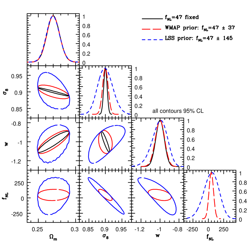
Figure 4.— Forecast marginalized likelihoods and $95\%$ C.L. contour plots from the cluster survey for the 4-parameter ($\Omega_{m}$, $\sigma_{8}$, $w$ and $f\!_{N\!L}$) model. In each contour plot, the other two parameters are marginalized over; in each likelihood plot, the other three parameters are marginalized over. We assume a fiducial $\Lambda$CDM model with $\sigma_{8}=0.9$ and use one mass bin defined by $M>M_{lim}=1.75\times 10^{14}\,h^{-1}\,{\rm M}_{\odot}$.

The major conclusion from Table 2 is that inclusion of a possible non-Gaussian component at the level allowed by present and future CMB constraints will not have an appreciable impact on the determination of dark energy parameters from cluster surveys. On the other hand, using only a single cluster mass bin (i.e., no information about the shape of the cluster mass function) and the WMAP prior on $f\!_{N\!L}$, the inclusion of non-Gaussianity degrades the cluster constraint on $\sigma_{8}$ by $50\%$. Moreover, using only the projected SDSS bispectrum constraint on $f\!_{N\!L}$, we do see degeneracies between $f\!_{N\!L}$ and dark energy: the error on $w$ from clusters increases by $\sim 70\%$, and the error on $\sigma_{8}$ grows by a factor of more than three compared to the purely Gaussian case. In all cases, the determination of $\Omega_{m}$ stays largely unaffected.

The expected degeneracy between $f\!_{N\!L}$ and $\sigma_{8}$ is evident from the two-parameter $95\%$ C.L. contour plots shown in Fig. 4, where we marginalized over the remaining parameters. The same overall behavior is observed when we impose priors on $\Omega_{m}$ and $\sigma_{8}$. In Fig. 4, the marginalized likelihood plot for $w$ shows that inclusion of the WMAP prior on $f\!_{N\!L}$ leads to essentially the same dark energy sensitivity for the cluster survey as one would have by fixing $f\!_{N\!L}$ (i.e., by not including non-Gaussianity).

Table 3 Same as Table 2 but with fiducial $\sigma_{8}=0.75$.

prior:	$\Delta f\!_{N\!L}=0$	$\Delta f\!_{N\!L}=5$	$\Delta f\!_{N\!L}=37$	$\Delta f\!_{N\!L}=145$
No priors
$\Delta w$	$0.079$	$0.079$ ($0\%$)	$0.083$ ($5\%$)	$0.124$ ($57\%$)
$\Delta\Omega_{m}$	$0.0140$	$0.0140$ ($0\%$)	$0.0140$ ($0\%$)	$0.0144$ ($3\%$)
$\Delta\sigma_{8}$	$0.0076$	$0.0076$ ($0\%$)	$0.0100$ ($32\%$)	$0.0238$ ($210\%$)
$\Delta f\!_{N\!L}$	-	$5.0$	$37$	$128$
Gaussian priors: $\Omega_{m}=0.27\pm 0.035$, $\sigma_{8}=0.75\pm 0.05$
$\Delta w$	$0.073$	$0.073$ ($0\%$)	$0.079$ ($8\%$)	$0.119$ ($63\%$)
$\Delta\Omega_{m}$	$0.0129$	$0.0129$ ($0\%$)	$0.0129$ ($0\%$)	$0.0129$ ($0\%$)
$\Delta\sigma_{8}$	$0.0070$	$0.0070$ ($0\%$)	$0.0094$ ($34\%$)	$0.0212$ ($200\%$)
$\Delta f\!_{N\!L}$	-	$5.0$	$37$	$118$
Gaussian priors: $\Omega_{m}=0.27\pm 0.0035$, $\sigma_{8}=0.75\pm 0.01$
$\Delta w$	$0.036$	$0.036$ ($0\%$)	$0.046$ ($28\%$)	$0.063$ ($75\%$)
$\Delta\Omega_{m}$	$0.0033$	$0.0033$ ($0\%$)	$0.0034$ ($3\%$)	$0.0034$ ($3\%$)
$\Delta\sigma_{8}$	$0.0021$	$0.0023$ ($10\%$)	$0.0054$ ($160\%$)	$0.0091$ ($330\%$)
$\Delta f\!_{N\!L}$	-	$5.0$	$32$	$56$
Fixed $\Omega_{m}=0.27$ and $\sigma_{8}=0.75$
$\Delta w$	$0.030$	$0.031$ ($3\%$)	$0.034$ ($10\%$)	$0.034$ ($10\%$)
$\Delta f\!_{N\!L}$	-	$4.2$	$7.5$	$7.6$

As far as the constraints on non-Gaussianity are concerned, the information provided by the cluster likelihood on $f\!_{N\!L}$ adds little to that from the CMB, while it mildly improves upon the non-Gaussianity constraints expected from the galaxy bispectrum. Even in the ideal case of perfect knowledge of $\Omega_{m}$ and $\sigma_{8}$, the expected error on $f\!_{N\!L}$ is $\Delta f\!_{N\!L}\simeq 6$, of the same order of the expected error from Planck.

We performed the same analysis for a fiducial $\sigma_{8}=0.75$, since this lower value has been recently suggested by CMB (Spergel et al., 2006) and cluster observations (Gladders et al., 2006; Dahle, 2006); as is well known, a lower clustering amplitude reduces the number of expected clusters and thereby reduces the constraining power of cluster surveys. The results are given in Table 3. In this case the total number of clusters for the fiducial model is about $6,000$; as a consequence, the cosmological constraints from the cluster survey are weaker than for the high-$\sigma_{8}$ model. However, the relative impact of the marginalization over primordial non-Gaussianity is reduced. This result can be expected since the effect of imposing the same priors on $f\!_{N\!L}$ is relatively smaller when the cosmological errors on the other parameters for the fixed $f\!_{N\!L}$ case increase.

To further illustrate the dependence of the results on survey parameters, in Table 4 we show the constraints obtained when the threshold cluster mass is reduced to $M_{lim}=1\times 10^{14}\,h^{-1}\,{\rm M}_{\odot}$. This lower threshold may be achieved, e.g., by supplementing SZ cluster detection with optical cluster selection using the red galaxy sequence (e.g. Gladders et al., 2006; Koester et al., 2006). In this case, the $4,000$ deg² survey to $z=1.5$ includes about $75,000$ clusters, and the forecast cosmological parameter errors (without non-Gaussianity) are smaller by almost a factor of two than for the case with larger $M_{lim}$ considered above. For this more sensitive cluster survey, the impact on cosmological parameters of marginalizing over $f\!_{N\!L}$ is correspondingly larger: while the impact on dark energy remains small, including non-Gaussianity with the WMAP prior expands the error on $\sigma_{8}$ by more than $100\%$.

As already discussed in the previous section, the degeneracy between $\sigma_{8}$ and $f\!_{N\!L}$ could be partially reduced by introducing a number of cluster mass bins and using the information contained in the shape of the mass function. In Table 5, we present the results for an analysis with a fiducial $\sigma_{8}=0.9$ and $M_{lim}=1.75\times 10^{14}\,h^{-1}\,{\rm M}_{\odot}$ as in Table 2 but subdividing the clusters into ten mass bins and using the likelihood function defined in Eq. (2.3). As the last column in Table 5 indicates the main effect of including mass bins is that the cluster constraint on the non-Gaussian parameter $f\!_{N\!L}$ becomes stronger than that from the SDSS galaxy bispectrum. Even without combining with external data sets one can reach a $1-\sigma$ error of $\Delta f\!_{N\!L}\simeq 50$, not too far from current limits from CMB observations. Further study would be needed to determine if this conclusion remains when realistic uncertainties in the cluster mass-observable relation are included in the analysis.

3.2. 2-parameter Dark Energy equation of state

Finally we consider the case of a time-varying dark energy equation of state (Chevallier & Polarski, 2001; Linder, 2003),

$$w(a)=w_{0}+(1-a)w_{a},$$ (20)

adding the parameter $w_{a}$ to the likelihood analysis studied so far. In this case the strong degeneracy between $w_{0}$ and $w_{a}$ enlarges considerably the region of parameter space that has to be covered for the likelihood function evaluation, including unphysical regions where the combination $w_{0}+w_{a}$, representing the equation of state at large redshift, takes large positive values. To avoid such cases we impose, by hand, a Gaussian prior on the value of $\Omega_{m}(z)$, requiring in particular $1-\Omega_{m}(z)<0.01$ at $1$-$\sigma$ at $z=30$, the initial redshift considered for the numerical solution to the differential equation governing the growth factor $D(z)$. This ensures that the Universe is matter-dominated at early times as required by structure growth.

Table 4 Same as Table 2 but with $M_{lim}=1\times 10^{14}\,h^{-1}\,{\rm M}_{\odot}$.

prior:	$\Delta f\!_{N\!L}=0$	$\Delta f\!_{N\!L}=5$	$\Delta f\!_{N\!L}=37$	$\Delta f\!_{N\!L}=145$
No priors on $\Omega_{m}$ and $\sigma_{8}$
$\Delta w$	$0.026$	$0.026$ ($0\%$)	$0.030$ ($15\%$)	$0.052$ ($100\%$)
$\Delta\Omega_{m}$	$0.0050$	$0.0050$ ($0\%$)	$0.0050$ ($0\%$)	$0.0052$ ($4\%$)
$\Delta\sigma_{8}$	$0.0031$	$0.0032$ ($3\%$)	$0.0066$ ($110\%$)	$0.0186$ ($500\%$)
$\Delta f\!_{N\!L}$	-	$5.0$	$36$	$113$
Gaussian priors: $\Omega_{m}=0.27\pm 0.035$, $\sigma_{8}=0.9\pm 0.05$
$\Delta w$	$0.026$	$0.026$ ($0\%$)	$0.030$ ($15\%$)	$0.050$ ($92\%$)
$\Delta\Omega_{m}$	$0.0050$	$0.0050$ ($0\%$)	$0.0050$ ($0\%$)	$0.0051$ ($2\%$)
$\Delta\sigma_{8}$	$0.0030$	$0.0031$ ($3\%$)	$0.0066$ ($120\%$)	$0.0174$ ($480\%$)
$\Delta f\!_{N\!L}$	-	$5.0$	$36$	$106$
Gaussian priors: $\Omega_{m}=0.27\pm 0.0035$, $\sigma_{8}=0.9\pm 0.01$
$\Delta w$	$0.017$	$0.017$ ($0\%$)	$0.023$ ($35\%$	$0.032$ ($88\%$)
$\Delta\Omega_{m}$	$0.0028$	$0.0028$ ($0\%$)	$0.0028$ ($0\%$)	$0.0028$ ($0\%$)
$\Delta\sigma_{8}$	$0.0018$	$0.0020$ ($11\%$)	$0.0051$ ($180\%$)	$0.0087$ ($380\%$)
$\Delta f\!_{N\!L}$	-	$5.0$	$32$	$56$
Fixed $\Omega_{m}=0.27$ and $\sigma_{8}=0.9$
$\Delta w$	$0.0100$	$0.0102$ ($2\%$)	$0.0102$ ($2\%$)	$0.0102$ ($2\%$)
$\Delta f\!_{N\!L}$	-	$3.1$	$4.0$	$4.0$

Table 5 Same as Table 2 but using 10 cluster mass bins.

prior:	$\Delta f\!_{N\!L}=0$	$\Delta f\!_{N\!L}=5$	$\Delta f\!_{N\!L}=37$	$\Delta f\!_{N\!L}=145$
No priors on $\Omega_{m}$ and $\sigma_{8}$
$\Delta w$	$0.044$	$0.044$ ($0\%$)	$0.046$ ($5\%$)	$0.048$ ($9\%$)
$\Delta\Omega_{m}$	$0.0082$	$0.0082$ ($0\%$)	$0.0083$ ($1\%$)	$0.0085$ ($4\%$)
$\Delta\sigma_{8}$	$0.0049$	$0.0050$ ($2\%$)	$0.0077$ ($57\%$)	$0.0103$ ($110\%$)
$\Delta f\!_{N\!L}$	-	$5.0$	$29$	$45$
Gaussian priors: $\Omega_{m}=0.27\pm 0.035$, $\sigma_{8}=0.9\pm 0.05$
$\Delta w$	$0.043$	$0.043$ ($0\%$)	$0.045$ ($5\%$)	$0.048$ ($12\%$)
$\Delta\Omega_{m}$	$0.0079$	$0.0079$ ($0\%$)	$0.0080$ ($1\%$)	$0.0082$ ($4\%$)
$\Delta\sigma_{8}$	$0.0048$	$0.0049$ ($2\%$)	$0.0075$ ($56\%$)	$0.0100$ ($110\%$)
$\Delta f\!_{N\!L}$	-	$5.0$	$29$	$45$
Gaussian priors: $\Omega_{m}=0.27\pm 0.0035$, $\sigma_{8}=0.9\pm 0.01$
$\Delta w$	$0.023$	$0.023$ ($0\%$)	$0.029$ ($26\%$)	$0.034$ ($48\%$)
$\Delta\Omega_{m}$	$0.0032$	$0.0032$ ($0\%$)	$0.0032$ ($0\%$)	$0.0032$ ($0\%$)
$\Delta\sigma_{8}$	$0.0021$	$0.0022$ ($5\%$)	$0.0048$ ($130\%$)	$0.0063$ ($200\%$)
$\Delta f\!_{N\!L}$	-	$5.0$	$26$	$35$
Fixed $\Omega_{m}=0.27$ and $\sigma_{8}=0.9$
$\Delta w$	$0.0166$	$0.0173$ ($4\%$)	$0.0181$ ($9\%$)	$0.0181$ ($9\%$)
$\Delta f\!_{N\!L}$	-	$3.7$	$5.5$	$5.5$

Table 6 Expected cosmological errors ($1\sigma$) from the cluster survey for the 5-parameter ($\Omega_{m}$, $\sigma_{8}$, $w_{0}$, $w_{a}$, $f\!_{N\!L}$) analysis. We assume a fiducial $\sigma_{8}=0.9$ and one mass bin defined by $M_{lim}=1.75\times 10^{14}\,h^{-1}\,{\rm M}_{\odot}$.

prior:	$\Delta f\!_{N\!L}=0$	$\Delta f\!_{N\!L}=5$	$\Delta f\!_{N\!L}=37$	$\Delta f\!_{N\!L}=145$
No priors on $\Omega_{m}$ and $\sigma_{8}$.
$\Delta w_{0}$	$0.195$	$0.195$ ($0\%$)	$0.196$ ($1\%$)	$0.208$ ($7\%$)
$\Delta w_{a}$	$0.73$	$0.73$ ($0\%$)	$0.74$ ($1\%$)	$0.87$ ($19\%$)
$\Delta\Omega_{m}$	$0.0156$	$0.0156$ ($0\%$)	$0.0158$ ($1\%$)	$0.0185$ ($19\%$)
$\Delta\sigma_{8}$	$0.0086$	$0.0087$ ($1\%$)	$0.0114$ ($32\%$)	$0.0296$ ($240\%$)
$\Delta f\!_{N\!L}$	-	$5.0$	$37$	$137$
Gaussian priors: $\Omega_{m}=0.27\pm 0.035$, $\sigma_{8}=0.9\pm 0.05$
$\Delta w_{0}$	$0.178$	$0.178$ ($0\%$)	$0.178$ ($0\%$)	$0.183$ ($3\%$)
$\Delta w_{a}$	$0.68$	$0.68$ ($0\%$)	$0.68$ ($0\%$)	$0.73$ ($7\%$)
$\Delta\Omega_{m}$	$0.0140$	$0.0140$ ($0\%$)	$0.0141$ ($1\%$)	$0.0151$ ($8\%$)
$\Delta\sigma_{8}$	$0.0078$	$0.0078$ ($0\%$)	$0.0105$ ($35\%$)	$0.0240$ ($210\%$)
$\Delta f\!_{N\!L}$	-	$5.0$	$37$	$118$
Gaussian priors: $\Omega_{m}=0.27\pm 0.0035$, $\sigma_{8}=0.9\pm 0.01$
$\Delta w_{0}$	$0.082$	$0.082$ ($0\%$)	$0.85$ ($4\%$)	$0.89$ ($9\%$)
$\Delta w_{a}$	$0.43$	$0.43$ ($0\%$)	$0.43$ ($0\%$)	$0.43$ ($0\%$)
$\Delta\Omega_{m}$	$0.0034$	$0.0034$ ($0\%$)	$0.0034$ ($0\%$)	$0.034$ ($0\%$)
$\Delta\sigma_{8}$	$0.0021$	$0.0023$ ($10\%$)	$0.0055$ ($160\%$)	$0.0091$ ($330\%$)
$\Delta f\!_{N\!L}$	-	$5.0$	$31$	$54$
Fixed $\Omega_{m}=0.27$ and $\sigma_{8}=0.9$
$\Delta w_{0}$	$0.068$	$0.069$ ($1\%$)	$0.071$ ($4\%$)	$0.071$ ($4\%$)
$\Delta w_{a}$	$0.37$	$0.039$ ($5\%$)	$0.40$ ($8\%$)	$0.40$ ($8\%$)
$\Delta f\!_{N\!L}$	-	$3.9$	$6.1$	$6.2$

In Table 6 we present the derived 1-$\sigma$ errors on the five parameters $\Omega_{m}$, $\sigma_{8}$, $w_{0}$ and $w_{a}$ with and without marginalization on $f\!_{N\!L}$ and assuming a single mass bin defined by $M>M_{lim}=1.75\times 10^{14}\,h^{-1}\,{\rm M}_{\odot}$. Since in this case the uncertainties on the parameters, which are sensitive to the strong $w_{0}$-$w_{a}$ degeneracy, are much larger than in the previous case, the effect of the marginalization on $f\!_{N\!L}$ with a CMB prior is even smaller than in the case of time-independent $w$. As before, however, marginalization over $f\!_{N\!L}$ with only the galaxy bispectrum prior substantially increases the error on $\sigma_{8}$.

As a final example, in Table 7 we consider parameter constraints in the time-varying dark energy cosmology using the ten cluster mass bins. As noticed earlier in the case of the 4-parameter analysis, the $\sigma_{8}$-$f\!_{N\!L}$ degeneracy is significantly reduced and the expected constraints on non-Gaussianity are still of the order of $\Delta f\!_{N\!L}\sim 50$.

4. Conclusions

The success of the $\Lambda$CDM standard cosmological model in recent years has been nothing short of spectacular. Upcoming surveys will either continue to confirm this model and constrain its parameters with unprecedented accuracy, or they will uncover discrepancies which will point the way toward improvements in our understanding of fundamental physics. Two questions addressing cosmology beyond the standard model that have been the subject of substantial attention in recent years are: what is the nature of the dark energy which is driving the accelerated expansion of the universe? and second, are fluctuations in the primordial matter distribution Gaussian, and therefore consistent with the predictions of the simplest inflationary models? In this paper, we obtain a rough estimate of the success that one of the most promising cosmological probes, galaxy cluster counts, is likely to have in answering these fundamental questions.

We have assumed an ideal cluster survey with survey parameters expected for the upcoming SPT and DES projects. Our fiducial cosmological model includes both dark energy and primordial non-Gaussianity using popular parameterized models, $w$ and $w_{a}$ for the former, and $f_{NL}$ for the latter. Cluster number counts as a function of mass, redshift, and cosmology were estimated using a standard fit to simulations (Jenkins et al., 2001), which we adjusted to allow for mild non-Gaussian initial conditions, and all clusters above a threshold mass were considered to be ”found” by our fiducial survey. We then performed a simple likelihood analysis on the cluster counts using priors from current WMAP and expected Planck and SDSS constraints on non-Gaussianity as well as approximate priors on the two other relevant cosmological parameters from other present and future data sets.

Our principal conclusion is that dark energy constraints are in all cases not substantially degraded by primordial non-Gaussianity when the model parameterized by the constant $f\!_{N\!L}$ and current limits from CMB observations are assumed. This is true despite the fact that variations in $f\!_{N\!L}$ close to current uncertainties induce differences in the mass function comparable in magnitude to variations of $10\%$ in the dark energy parameter $w$. A stronger degeneracy is observed instead between $f\!_{N\!L}$ and $\sigma_{8}$; in this case, the expected errors on $\sigma_{8}$ from future cluster surveys can be noticeably affected when non-Gaussianity is included in the analysis.

Table 7 Same as Table 6 but using 10 cluster mass bins.

prior:	$\Delta f\!_{N\!L}=0$	$\Delta f\!_{N\!L}=5$	$\Delta f\!_{N\!L}=37$	$\Delta f\!_{N\!L}=145$
No priors on $\Omega_{m}$ and $\sigma_{8}$.
$\Delta w_{0}$	$0.180$	$0.180$ ($0\%$)	$0.186$ ($3\%$)	$0.197$ ($9\%$)
$\Delta w_{a}$	$0.68$	$0.68$ ($0\%$)	$0.71$ ($4\%$)	$0.78$ ($15\%$)
$\Delta\Omega_{m}$	$0.0141$	$0.0141$ ($0\%$)	$0.0151$ ($7\%$)	$0.0170$ ($21\%$)
$\Delta\sigma_{8}$	$0.0078$	$0.0079$ ($1\%$)	$0.0113$ ($45\%$)	$0.0158$ ($100\%$)
$\Delta f\!_{N\!L}$	-	$5.0$	$31$	$51$
Gaussian priors: $\Omega_{m}=0.27\pm 0.035$, $\sigma_{8}=0.9\pm 0.05$
$\Delta w_{0}$	$0.167$	$0.168$ ($1\%$)	$0.170$ ($2\%$)	$0.175$ ($5\%$)
$\Delta w_{a}$	$0.64$	$0.64$ ($0\%$)	$0.66$ ($3\%$)	$0.70$ ($9\%$)
$\Delta\Omega_{m}$	$0.0129$	$0.0130$ ($1\%$)	$0.0136$ ($5\%$)	$0.0146$ ($13\%$)
$\Delta\sigma_{8}$	$0.0072$	$0.0073$ ($1\%$)	$0.0103$ ($43\%$)	$0.0138$ ($92\%$)
$\Delta f\!_{N\!L}$	-	$5.0$	$30$	$48$
Gaussian priors: $\Omega_{m}=0.27\pm 0.0035$, $\sigma_{8}=0.9\pm 0.01$
$\Delta w_{0}$	$0.081$	$0.081$ ($0\%$)	$0.83$ ($2\%$)	$0.84$ ($4\%$)
$\Delta w_{a}$	$0.42$	$0.42$ ($0\%$)	$0.42$ ($0\%$)	$0.42$ ($0\%$)
$\Delta\Omega_{m}$	$0.0033$	$0.0033$ ($0\%$)	$0.0033$ ($0\%$)	$0.033$ ($0\%$)
$\Delta\sigma_{8}$	$0.0021$	$0.0023$ ($10\%$)	$0.0049$ ($130\%$)	$0.0063$ ($200\%$)
$\Delta f\!_{N\!L}$	-	$5.0$	$26$	$35$
Fixed $\Omega_{m}=0.27$ and $\sigma_{8}=0.9$
$\Delta w_{0}$	$0.067$	$0.068$ ($1\%$)	$0.070$ ($4\%$)	$0.070$ ($4\%$)
$\Delta w_{a}$	$0.37$	$0.038$ ($3\%$)	$0.40$ ($8\%$)	$0.40$ ($8\%$)
$\Delta f\!_{N\!L}$	-	$3.8$	$5.9$	$6.0$

A secondary conclusion is that the cluster survey itself might have sufficient statistical power to provide a valuable cross check on any detection or non-detection of primordial non-Gaussianity in CMB experiments, particularly when information on the cluster distribution as a function of the mass is taken into account.

However, we must emphasize that we have not attempted to include in our analysis any of the systematic and statistical errors in the clusters mass determination, which are likely to cause trouble for real surveys, as well as uncertainties on the predictions for the mass function, and our results must be interpreted with this in mind. We believe that our principal result should be quite robust, since any significant increase in the error budget will reduce constraining power on dark energy parameters and de-emphasize the confusion caused by any non-Gaussian initial conditions. On the other hand, the effectiveness of clusters as a cross check of primordial non-Gaussianity estimates from the CMB could be dramatically worsened, and should therefore be the subject of future work.

References

- Abbott et al. (2005) Abbott, T., et al. 2005, astro-ph/0510346
- Acquaviva et al. (2003) Acquaviva, V., Bartolo, N., Matarrese, S., & Riotto, A. 2003, Nucl. Phys., B667, 119
- Alishahiha et al. (2004) Alishahiha, M., Silverstein, E., & Tong, D. 2004, Phys. Rev., D70, 123505
- Amara & Refregier (2004) Amara, A., & Refregier, A. 2004, Mon. Not. Roy. Astron. Soc., 351, 375
- Arkani-Hamed et al. (2004) Arkani-Hamed, N., Creminelli, P., Mukohyama, S., & Zaldarriaga, M. 2004, JCAP, 0404, 001
- Bartolo et al. (2004) Bartolo, N., Komatsu, E., Matarrese, S., & Riotto, A. 2004, Phys. Rept., 402, 103
- Battye & Weller (2003) Battye, R. A., & Weller, J. 2003, Phys. Rev., D68, 083506
- Benson et al. (2002) Benson, A. J., Reichardt, C., & Kamionkowski, M. 2002, Mon. Not. Roy. Astron. Soc., 331, 71
- Chen & Szapudi (2006) Chen, G., & Szapudi, I. 2006, astro-ph/0606394
- Chevallier & Polarski (2001) Chevallier, M., & Polarski, D. 2001, Int. J. Mod. Phys., D10, 213
- Chiu et al. (1998) Chiu, W. A., Ostriker, J. P., & Strauss, M. A. 1998, Astrophys. J., 494, 479
- Colafrancesco et al. (1989) Colafrancesco, S., Lucchin, F., & Matarrese, S. 1989, Astrophys. J., 345, 3
- Creminelli (2003) Creminelli, P. 2003, JCAP, 0310, 003
- Creminelli et al. (2006) Creminelli, P., Nicolis, A., Senatore, L., Tegmark, M., & Zaldarriaga, M. 2006, JCAP, 0605, 004
- Crocce et al. (2006) Crocce, M., Pueblas, S., & Scoccimarro, R. 2006, submitted to Mon. Not. Roy. Astron. Soc., astro-ph/0606505
- Dahle (2006) Dahle, H. 2006, submitted to Astrophys. J., astro-ph/0608480
- Dvali et al. (2004) Dvali, G., Gruzinov, A., & Zaldarriaga, M. 2004, Phys. Rev., D69, 023505
- Ebeling et al. (1996) Ebeling, H., et al. 1996, Mon. Not. Roy. Astron. Soc., 281, 799
- Feldman et al. (2001) Feldman, H. A., Frieman, J. A., Fry, J. N., & Scoccimarro, R. 2001, Phys. Rev. Lett., 86, 1434
- Francis et al. (2005) Francis, M. R., Bean, R., & Kosowsky, A. 2005, JCAP, 0512, 001
- Gladders et al. (2006) Gladders, M. D., et al. 2006, astro-ph/0603588
- Haiman et al. (2000) Haiman, Z., Mohr, J. J., & Holder, G. P. 2000, Astrophys. J., 553, 545
- Heitmann et al. (2005) Heitmann, K., Ricker, P. M., Warren, M. S., & Habib, S. 2005, Astrophys. J. Suppl., 160, 28
- Henry (1997) Henry, J. P. 1997, Astrophys. J., 489, L1
- Henry & Arnaud (1991) Henry, J. P., & Arnaud, K. A. 1991, Astrophys. J., 372, 410
- Holder et al. (2001) Holder, G., Haiman, Z., & Mohr, J. 2001, Astrophys. J., 560, L111
- Hu (2003) Hu, W. 2003, Phys. Rev., D67, 081304
- Hu & Kravtsov (2003) Hu, W., & Kravtsov, A. V. 2003, Astrophys. J., 584, 702
- Huterer et al. (2004) Huterer, D., Kim, A., Krauss, L. M., & Broderick, T. 2004, Astrophys. J., 615, 595
- Huterer & Linder (2006) Huterer, D., & Linder, E. V. 2006, astro-ph/0608681
- Jenkins et al. (2001) Jenkins, A., et al. 2001, Mon. Not. Roy. Astron. Soc., 321, 372
- Koester et al. (2006) Koester, B., et al. 2006, submitted to Astrophys J.
- Kolb et al. (2006) Kolb, E. W., Riotto, A., & Vallinotto, A. 2006, Phys. Rev., D73, 023522
- Komatsu & Spergel (2001) Komatsu, E., & Spergel, D. N. 2001, Phys. Rev., D63, 063002
- Komatsu et al. (2003) Komatsu, E., et al. 2003, Astrophys. J. Suppl., 148, 119
- Koyama et al. (1999) Koyama, K., Soda, J., & Taruya, A. 1999, Mon. Not. Roy. Astron. Soc., 310, 1111
- Kravtsov et al. (2006) Kravtsov, A. V., Vikhlinin, A., & Nagai, D. 2006, submitted to Astrophys. J., astro-ph/0603205
- Levine et al. (2002) Levine, E. S., Schulz, A. E., & White, M. J. 2002, Astrophys. J., 577, 569
- Liguori et al. (2006) Liguori, M., Hansen, F. K., Komatsu, E., Matarrese, S., & Riotto, A. 2006, Phys. Rev., D73, 043505
- Lima & Hu (2004) Lima, M., & Hu, W. 2004, Phys. Rev., D70, 043504
- Lima & Hu (2005) —. 2005, Phys. Rev., D72, 043006
- Linder (2003) Linder, E. V. 2003, Phys. Rev. Lett., 90, 091301
- Lucchin & Matarrese (1988) Lucchin, F., & Matarrese, S. 1988, Astrophys. J., 330, 535
- Lyth et al. (2003) Lyth, D. H., Ungarelli, C., & Wands, D. 2003, Phys. Rev., D67, 023503
- Majumdar & Mohr (2003) Majumdar, S., & Mohr, J. J. 2003, Astrophys. J., 585, 603
- Majumdar & Mohr (2004) —. 2004, Astrophys. J., 613, 41
- Maldacena (2003) Maldacena, J. M. 2003, JHEP, 05, 013
- Marian & Bernstein (2006) Marian, L., & Bernstein, G. M. 2006, Phys. Rev., D73, 123525
- Matarrese (2006) Matarrese, S. 2006, private communication
- Matarrese et al. (2000) Matarrese, S., Verde, L., & Jimenez, R. 2000, Astrophys. J., 541, 10
- Mathis et al. (2004) Mathis, H., Diego, J. M., & Silk, J. 2004, Mon. Not. Roy. Astron. Soc., 353, 681
- Molnar et al. (2004) Molnar, S. M., Haiman, Z., Birkinshaw, M., & Mushotzky, R. F. 2004, Astrophys. J., 601, 22
- Perlmutter et al. (1999) Perlmutter, S., et al. 1999, Astrophys. J., 517, 565
- Pierpaoli et al. (2003) Pierpaoli, E., Borgani, S., Scott, D., & White, M. J. 2003, Mon. Not. Roy. Astron. Soc., 342, 163
- PLANCK (2006) PLANCK. 2006, the Planck collaboration, ”Planck: The scientific programme”, astro-ph/0604069
- Press & Schechter (1974) Press, W. H., & Schechter, P. 1974, Astrophys. J., 187, 425
- Rapetti et al. (2005) Rapetti, D., Allen, S. W., & Weller, J. 2005, Mon. Not. Roy. Astron. Soc., 360, 555
- Reed et al. (2006) Reed, D., Bower, R., Frenk, C., Jenkins, A., & Theuns, T. 2006, submitted to Mon. Not. Roy. Astron. Soc., astro-ph/0607150
- Riess et al. (1998) Riess, A. G., et al. 1998, Astron. J., 116, 1009
- Robinson & Baker (2000) Robinson, J., & Baker, J. E. 2000, Mon. Not. Roy. Astron. Soc., 311, 781
- Robinson et al. (1998) Robinson, J., Gawiser, E., & Silk, J. 1998, astro-ph/9805181
- Robinson et al. (2000) —. 2000, Astrophys. J., 532, 1
- Ruhl et al. (2004) Ruhl, J. E., et al. 2004, the SPT collaboration, astro-ph/0411122
- Sadeh et al. (2006) Sadeh, S., Rephaeli, Y., & Silk, J. 2006, Mon. Not. Roy. Astron. Soc., 368, 1583
- Sasaki et al. (2006) Sasaki, M., Valiviita, J., & Wands, D. 2006, astro-ph/0607627
- Scoccimarro et al. (2004) Scoccimarro, R., Sefusatti, E., & Zaldarriaga, M. 2004, Phys. Rev., D69, 103513
- Seljak (2002) Seljak, U. 2002, Mon. Not. Roy. Astron. Soc., 337, 769
- Seljak & Zaldarriaga (1996) Seljak, U., & Zaldarriaga, M. 1996, Astrophys. J., 469, 437
- Spergel et al. (2006) Spergel, D. N., et al. 2006, submitted to Astrophys. J. Suppl., astro-ph/0603449
- Verde et al. (2000) Verde, L., Wang, L.-M., Heavens, A., & Kamionkowski, M. 2000, Mon. Not. Roy. Astron. Soc., 313, L141
- Wang et al. (2004) Wang, S., Khoury, J., Haiman, Z., & May, M. 2004, Phys. Rev., D70, 123008
- Warren et al. (2006) Warren, M. S., Abazajian, K., Holz, D. E., & Teodoro, L. 2006, Astrophys. J., 646, 881
- White (1999) White, M. J. 1999, Mon. Not. Roy. Astron. Soc., 310, 511
- Willick (2000) Willick, J. A. 2000, Astrophys. J., 530, 80
- Zaldarriaga (2004) Zaldarriaga, M. 2004, Phys. Rev., D69, 043508