Abundances of Baade’s Window Giants from Keck/HIRES Spectra: II. The Alpha- and Light Odd Elements

Abstract

We report detailed chemical abundance analysis of 27 RGB stars towards the Galactic bulge in Baade’s Window for elements produced by massive stars: O, Na, Mg, Al, Si, Ca and Ti. All of these elements are overabundant in the bulge relative to the disk, indicating that the bulge is enhanced in Type II supernova ejecta and most likely formed more rapidly than the disk.

Our [Mg/Fe] ratios, confirmed by [Al/Mg], declines much more slowly with [Fe/H] than O, Si, Ca and Ti. The [Mg/Fe] ratio stays above +0.25 dex up to well above solar metallicity. We attribute the rapid decline of [O/Fe] to a metallicity-dependent modulation of the oxygen yield from massive stars, perhaps connected to the Wolf-Reyet phenomenon.

The explosive nucleosynthesis alphas, Si, Ca and Ti, relative to Fe, possess identical trends with [Fe/H], consistent with their putative common origin. We note that different behaviors of hydrostatic and explosive alpha elements can be seen in the stellar abundances of stars in Local Group dwarf galaxies. We also attribute the decline of Si,Ca and Ti, relative to Mg, to metallicity-dependent yields for these explosive alpha elements from Type II supernovae. The production of explosive alphas in Type Ia supernovae likely explains the absence of obvious difference between Mg and Si, Ca, Ti trends in the Galactic thin disk.

An alternative explanation for the [Mg/$<$SiCaTi$>$] increase with metallicity is an excess population of 30–35M_⊙ stars in the bulge that grew in importance with [Fe/H]. In this model the bulge formation timescale would have been significantly longer than our favored scenario of declining metallicity-dependent yields from Type II supernovae.

The starkly smaller scatter of [$<$SiCaTi$>$/Fe] with [Fe/H] in the bulge, as compared to the halo, is consistent with expected efficient mixing for the bulge. Since the metal-poor bulge [$<$SiCaTi$>$/Fe] ratios are higher than $\sim$80% of the halo, the early bulge could not have formed from gas with the present-day halo composition. If the bulge formed from halo gas, it occurred before $\sim$80% of today’s stellar halo; and the halo subsequently reduced its alpha/Fe ratios significantly.

The lack of overlap between the thick and thin disk composition with the bulge does not support the idea that the bulge was built by a thickening of the disk driven by the bar.

The trend of [Al/Fe] is very sensitive to the chemical evolution environment: a comparison of the bulge, disk and Sagittarius dwarf spheroidal galaxy shows a range of $\sim$0.7 dex in [Al/Fe] at a given [Fe/H]; presumably due to a range of Type II/Type Ia supernova ratios in these systems.

1. Introduction

We present the second in a series of papers on the abundances of a sample of Galactic bulge K giants. While our long term aim is to undertake a large scale survey of the Galactic bulge, the first step is to determine the correct stellar abundance scale. This is straightforward for most stellar populations, but has been a subject of debate for bulge and metal rich stars. Paper I (Fulbright et al., 2006a; hereafter Paper I) reports our new iron abundance scale that supersedes (McWilliam & Rich, 1994; hereafter MR94). Here we employ our new iron abundance scale to derive the abundances of alpha elements in the Galactic bulge stars. In the third paper, we turn to the iron peak, r-, and s-process elements. In future papers we will use the methods developed here to extend our studies to larger samples using multiobject spectroscopy. The initial aim is to settle the iron abundance scale and then to follow with well determined abundances for a large number of additional elements. When issues concerning the abundance determination of these additional elements have been settled, it will be possible to investigate large samples with confidence.

The understanding that it is possible for stellar populations to be both old and metal rich was gained surprisingly early. In referring to the bulge of M31, Baade (1963) states “And the process of enrichment has taken very little time. … So the CN giants that contribute most of the light in the nuclear region of the Nebula must also be called old stars; they are not young”. The journey from insight to demonstration took nearly four decades, however. Some significant steps along the way include the first integrated light spectroscopy of the bulge (Whitford, 1978), surveys of bulge M giants (Blanco & Blanco, 1984) the first survey of bulge K giants (Rich, 1988), the first detailed abundances in the Galactic bulge (MR94), and the first demonstration that the bulge is as old as metal rich globular clusters (Ortolani et al., 1995). Recent studies that confirm the old, metal rich nature of the bulge population (Kuijken & Rich, 2002; Zoccali et al., 2003), and most recently, the revised bulge abundance scale (Paper I).

The events leading to the development of the new iron abundance scale are reviewed in Paper I and in Rich et al. (2006). Our new abundance scale is based on the use of weak iron lines in Arcturus (HR3905); we can use the very well-constrained parameters for Arcturus to perform a differential analysis, which effectively cancels out systematic problems with $gf$-values and stellar atmospheres. The adopted lines are weak enough to remain on the linear portion of the curve of growth even for our most metal rich Galactic bulge giants. The second advance is the use of multiple approaches to assess bulge membership and stellar parameters; this effort overcomes earlier problems with self-consistent abundance analysis that did not rely on photometry.

A significant thread in the abundance studies has been the discovery that alpha elements are enhanced in bulge giants. This was demonstrated convincingly for the case of Mg and Ti (and to some extent Na and Al) in MR94. Preliminary studies of high resolution spectra obtained at Keck, based on the MR94 iron abundance scale and line list, confirmed the Mg enhancement and found all alpha elements enhanced (Rich & McWilliam, 2000; hereafter RM00; McWilliam & Rich, 2004; hereafter MR04). It is widely accepted that at least Mg is enhanced in extragalactic spheroidal populations (Worthey et al., 1992). The modern effort to revisit Whitford’s (1978) spectroscopy of the integrated light of a Galactic bulge field compared to external galaxies (Puzia et al., 2002) supports moderate alpha enhancement in the bulge and shows that the bulge falls on the lower end of the elliptical galaxy sequence.

The long standing operating paradigm is that alpha elements (e.g. O, Mg, Si, Ca) are produced in the supernovae of short lived massive stars while iron is predominantly produced in core collapse SNe that occur on a timescale that is 1-2 orders of magnitude longer (Tinsley, 1979; Weaver et al., 1989; Timmes et al., 1995; McWilliam, 1997). Matteucci & Brocato (1990) combined the SN yields and sophisticated chemical evolution models. Matteucci et al. (1999) employ the SN yields of Thielemann et al. (1996) for Type Ia and Woosley & Weaver (1995) for Type II SNe. The yields from numerical models of SNe, along with corroborating abundance determinations in very metal poor stars, are the theoretical underpinning that support this paradigm. The models of Matteucci & Brocato (1990), Matteucci et al. (1999), and Ballero et al. (2006) incorporate star formation predictions and the requirement that the bulge form rapidly ($<1$ Gyr). The alpha enhancement has been known since MR94 and is the constraint (along with the observations of an old turnoff age) that underpin the empirical arguments for a very old Galactic bulge.

The growing evidence that the Galactic bulge formed early and rapidly finds support in numerous observations at high redshift. The discovery of the Lyman break selected high redshift galaxy population by Steidel et al. (1996) was the first direct identification of a population of galaxies at $z>3$ with high star formation rates and the potential (in terms of mass) to evolve into galaxies like the Milky Way. Since that discovery there have been numerous other high redshift populations discovered that are equally plausible bulge progenitors; all share the property of having high rates of star formation and large stellar mass. Steidel et al. (1996) and Adelberger et al. (2003) have also detected and studied metal enriched wind outflows from Lyman Break galaxies. Pettini et al. (2002) find winds and derive alpha enhancements in a gravitationally lensed Lyman break galaxy observed at high spectral resolution. These offer additional evidence of high star formation and also indicate that winds should eventually be incorporated into the chemical evolution models. However, the evolutionary path of these high redshift galaxies cannot unequivocally link them to a Milky Way like result in the present day Universe.

The union of these ideas–that there is overwhelming evidence for a rapid formation timescale for the bulge both from the chemical enrichment, turnoff age, and high redshift perspectives, is described in Rich et al. (2006). If the bulge has undergone secular evolution (Kormendy & Kennicutt, 1994) then it has done so (it would seem) mostly in the dynamical sense, with its population having been built early and rapidly. However, in the case of the bulge, as opposed to giant ellipticals, there are good reasons to suspect that the starburst formation scenario (Elmegreen, 1999) is not the complete picture. Immeli et al. (2004) explore models in which the bulge forms from the accumulation of smaller units (as might be favored in the LCDM cosmology scenario). It may be possible to detect fossil evidence of these subclumps by correlations between abundance and kinematics, or differing element trends (e.g. [Mg/Fe] vs [Fe/H] at a different level). A large scale survey program to study these trends will require significant samples of stars with abundances determined to very high precision. Contamination by the thick disk and foreground disk could mimic the expected signal from a subclump. Further, it should be noted that the bar, a rapid formation timescale, and high metallicity all point toward a formation model in which the mass is in place early; nonetheless, scenarios of inhomogeneous evolution should be explored with larger surveys.

Evidence for the presence of a bar structure in the bulge is now indisputable. Observations by the COBE satellite and subsequent modeling (Dwek et al., 1995) argue for the bar based on surface photometry. Mao & Paczynski (2002) find evidence for the bar from the stellar population and from stellar dynamics (Zhao et al., 1994). A recent study (Soto Vicencio et al., 2006) finds that kinematics consistent with the bar set in at [Fe/H]$>-0.2$, with more metal poor stars being more consistent with an isotropic velocity ellipsoid. Bars are also thought to be formed by secular evolution (Kormendy & Kennicutt, 1994). There has been extensive theoretical discussion about the origin of the bar based on dynamical processes that are secular in nature (Combes, 2001). There is prima facie evidence for ongoing star formation in the nuclear region and modeling of the luminosity function in fields within 50 pc of the nucleus requires a constant star formation rate, with models dominated by early bursts of formation are ruled out by models of the luminosity function Figer et al. (2004). A study of infrared abundances in old stars in the bulge by Ramiŕez et al. (2000) finds no abundance gradient from latitude 0^o to -$6^{\rm o}$, an observation expected if secular evolution is an important process in establishing the vertical thickness of the bar. At present, there is strong evidence from the turnoff age and chemical evolution that the bulge formed early and rapidly. On the other hand, the bulge has been shown to have a clear bar structure and other properties (no vertical abundance gradient) more consistent with secular evolution.

There is at present a conflicted situation with regards to age and formation constraints from the turnoff and chemistry, and possible secular evolution from the presence of the bar structure. We believe that it is vital to not only measure abundances of alpha elements in a larger sample, but to also measure the abundances of more species, so as to provide better constraints for the chemical evolution models. We have the opportunity in the bulge to track the abundance trends of many elements in detail. This is something that we will be unlikely to achieve for any other spheroidal population in the near future. This approach can be used to ask more detailed questions, such as constraints on the initial mass function as well as setting limits on the timescale of the formation epoch to greater precision. The presence or absence of vertical gradients in the alphas and [Fe/H] gives an additional important constraint on whether secular processes have played a role in the formation of the bulge.

We also undertake a detailed comparison between the bulge and thick disk/halo. These well studied populations serve both as test samples to confirm the soundness of our abundance analysis and as a comparison sample against which the bulge abundance patterns can be compared. This will enable us to relate our findings in the bulge to the formation of well studied populations in the Milky Way.

The paper is organized as follows. In Section 2, we discuss the spectral data and the creation of a new unblended line list for the elements under study. We review the stellar parameters adopted for these stars and their uncertainties in Section 3. In Section 4, we describe the uncertainties of our abundance determinations, including a full quantitative analysis method. In Section 5, we apply a simple correction for the varying alpha-enhancements of our target stars. In Section 6, we check our abundance results, showing that our adopted parameters return abundances in ionization equilibrium and in agreement with previous literature studies. Our primary bulge abundance results are presented in Section 7, which includes the evidence for enhanced alpha element ratios at all metallicities in the bulge. Further discussion of the abundances of Na and Al are in Section 8, including evidence that the Type II SNe that enriched the bulge included some metal-rich stars. In Section 9, we find that the metal-poor stars in the bulge show the same Na-O anticorrelation as seen in metal-poor globular clusters and discuss what that may mean for the early formation of the bulge.

2. Data and Line List

The spectra used in this work are the same as those used in Paper I. Briefly, most of the bulge star spectra were obtained with the Keck I telescope using the HIRES echelle spectrograph (Vogt et al., 1994) at a resolution of either 45,000 or 67,000. Most of the disk giant spectra were obtained with the echelle spectrograph on the Las Campanas Observatory 2.5-m du Pont telescope. The disk giant spectra were of higher signal-to-noise, but of lower resolution (roughly 30,000). We use the same continuum values as defined in that work, and we continue to use the GETJOB program (McWilliam et al., 1995) to measure equivalent width values and their uncertainties.

An adjustment to our line-measurement methods was required around the Ca auto-ionization features at 6319, 6444 and 6362 Å (Griffin, 1964; Mitchell & Mohler, 1965). These features are broad, several Ångstroms wide, and relatively shallow. For the Mg I lines near 6319Å, within one of these features, we measured modified equivalent widths using the IRAF splot package, with the Ca auto-ionization line profile treated as continuum. A full abundance analysis treatment of these lines would include the blend of the Ca auto-ionization feature with the Mg I line profiles; this would require modification of the spectrum synthesis code MOOG, and a reliable Ca auto-ionization lifetime for the lower level. Since these options were not presently available to us, and because the Ca auto-ionization feature is quite shallow, we employ the first-order approximation for the analysis: namely, to treat the modified equivalent widths as normal EWs without the Ca autoionization line. This approximation should work well when both the autoionization line and the target, Mg I, line are unsaturated. During the abundance analysis stage, we have found that lines measured this way yield abundances that agree with other, unaffected, lines of the same species.

In order to identify unblended lines useful for abundance analysis we employ the method used to find clean Fe lines in Paper I: spectrum synthesis was performed for all lines between 5000 and 8000 Å using the Kurucz atomic line list plus the CN line list of MR94 for for Arcturus (HR5340), the Sun, and $\mu$ Leo (HR3905). For every line we calculated the log(RW) value and compared it to the log(RW) value for the sum of all lines within 0.2 Å of the line center. Lines were then sorted in order of relative contamination to find the most unblended lines for each species.

Inspection of the spectral atlases of Arcturus (Hinkle et al., 2000) and the Sun (Kurucz, 1993) and our Paper I spectrum of $\mu$ Leo were performed to eliminate lines blended with unknown features, including telluric contamination. Additionally, we cut lines that are too strong ($>200$ mÅ in the $\mu$ Leo synthesis, assuming solar ratios) or too weak ($<5$ mÅ in the Arcturus synthesis, again assuming solar ratios). In practice, we rarely used lines approaching these limits in the final analysis, but we wished to be inclusive at this point in order to account for possible errors in the Kurucz line list gf-values, non-solar abundance ratios, etc. For the purpose of identifying unblended lines we did not include hyperfine splitting for Na or Al lines.

For these initial analyses, we used a Kurucz model atmospheres with overshooting. For each target line, we include the blending effects for any weak lines within 0.2 Å. The synthesis needed to remove these blending effects assumed solar element ratios with the exception of assuming [C/Fe] = $-0.2$ and [N/Fe] = +0.4. These revised C and N abundances reflect the effects of dredge up on the red giant branch (Lambert & Ries, 1981) and will increase the strength of CN features blended with the features of interest. We attempted to find lines where the contaminants contributed less than 0.05 dex to the final line log(RW) in the synthesis of $\mu$ Leo.

Several of the Mg I lines are actually blends of three Mg I lines at nearly identical (within 0.01 Å) wavelengths. The weaker lines usually have gf-values at least a factor of 10 weaker than the strongest line, but we retain the weaker lines in the deblending routine.

Other lines (such as the Na I lines at 5682 Å and 5688 Å) have very close blends, but we are forced to use these lines because other options are not available (the 6154 Å and 6160 Å Na I lines were not in the wavelength coverage of every star). In such cases, we use the “blends” package of MOOG (Sneden, 1973) to deblend the full equivalent width of the whole blend. The line parameters of the other features in the blend were taken from the Kurucz line list. For the 27 Baade’s Window stars where at least one line of both doublets were used we found a mean difference of $-0.01\pm 0.09$ (standard deviation) where the value given by the redder doublet was slightly larger. For the 6300 Å [O I] line we included the Ni I blend (Allende Prieto et al., 2001), even though its effect is negligible in giants.

As in Paper I, we will use Arcturus as the reference star for our differential analysis. The advantage of a line-by-line differential analysis is that systematic errors, due to various inadequacies of the model atmospheres, such as non-plane parallel geometry, 3D hydrodynamical variations, chromospheric effects, non-LTE, magnetic fields etc, may to a first approximation, cancel out when performed relative to similar stars; certainly the oscillator strengths of the atomic lines do not enter into the abundance determinations.

To place our abundances on an absolute scale, we must adopt $\log{\epsilon}$ values for Arcturus for every element. Our method for determining these abundance values is similar to the method we used in Paper I to determine the $\log{\epsilon}$(Fe) abundance. Errors in these determinations will create a systematic zero-point offset for each element.

We start with a line list as constructed above, but we change our selection criteria to only exclude lines that show any blending in both the Sun and Arcturus. This adds a few lines that are blended or too strong in $\mu$ Leo, but we exclude many lines that have minor blends that were allowed into the main list. The equivalent width (EW) values for these lines were measured in both the Hinkle et al. (2000) Arcturus atlas and the Kurucz et al. (1984) solar atlas.

The measured line lists were then run through the MOOG stellar abundance program using a model atmosphere appropriate for Arcturus: a Fiorella Castelli alpha-enhanced AODFNEW atmosphere with T_eff = 4290 K, log $g$ = 1.55, [m/H] = $-$0.50, and v_t = 1.67 km/s. For the Sun we used a Castelli solar-ratio ODFNEW atmosphere with T_eff = 5770K, log $g$ = 4.44, [m/H] = 0.00, and v_t = 0.93 km/s. A line-by-line differential analysis was conducted which yields the relative abundance of Arcturus with respect to the Sun. The Arcturus abundances were then placed on an absolute scale by the use of Lodders (2003) solar abundance ratios, with the exception that we continue to use the solar $\log{\epsilon}$(Fe) value of 7.45 we derive in Paper I. The EW values of the lines used in this analysis are given in Table 1 and the final adopted Arcturus abundances are given in Table 2. The final line list is given in Table 3. Our EW measurements are given in Table 4.

3. Stellar Parameters and Parameter Errors

Paper I gives our approach for deriving the stellar parameters for our program stars. In Paper I, we mainly used Kurucz atmospheres with overshooting enabled, but in this paper we will use the Castelli model atmospheres in order to create a simple correction for the variable [$\alpha$/Fe] ratios found in our stars (see Section 5 for the description of the correction).

The parameter-finding methods using the alternate atmosphere models are exactly the same as performed in Paper I. The choice of atmosphere grid has a small effect on the final adopted parameters (see Table 9 of Paper I). We list the final adopted parameters for each grid for each star in Table 5.

In this paper, we will derive uncertainties for our abundance measurements using a method based on the work of McWilliam et al. (1995). One component of the error analysis is deriving the uncertainties in the stellar parameters. The listed ($\sigma$T) value is the standard deviation of the three (or two for a few stars mentioned in Section 7 of Paper I) T_eff values derived by the three different T_eff-setting methods. The $\sigma$[m/H] value comes from the standard deviation of the Fe I lines used to measure the [Fe/H] abundance. It would be more correct to use the derived value of $\sigma$[Fe I/H] for $\sigma$[m/H] (and therefore make this an iterative process), but we found from experience that using the less exact standard deviation value makes minimal difference. The standard deviation of the Fe I lines ends up being slightly larger than the weighted error for these lines. The $\sigma$v_t value comes from Equation 2 from Paper I.

The value of $\sigma$log $g$ required a Monte Carlo simulation. The derived log $g$ values come from Equation 1 in Paper I, where log $g$ is a function of stellar mass, T_eff, and M_bol. The error in M_bol depends on photometry, reddening, distance and bolometric correction uncertainties. We use the bolometric corrections of Alonso et al. (1999), which give BC(V) as a function of T_eff and [m/H]. While it would be possible to use normal analytical propagation of error techniques to calculate $\sigma$log $g$, we decided to use a Monte Carlo simulation to assure there were no hidden dependencies.

To simplify the analysis, we adopted standard values for the uncertainties of several of the inputs. For the bulge sample, we assume: $\sigma$M$=0.1$ M_⊙, $\sigma$V$=0.05$ mag, and $\sigma$A${}_{\rm V}=0.10$ mag. We assume a distance error of about 500 pc, which converts to a distance modulus uncertainty of 0.13 mag. We include the stated fitting uncertainty of 0.024 mag to the BC(V) function of Alonso et al. (1999). For the disk giant sample, we set the distance and A_V errors to zero. Therefore, the main variation in the value of $\sigma$log $g$ between stars is due the the differences in T_eff, $\sigma$T, [m/H] and $\sigma$[m/H].

The values of $\sigma$T for individual stars was calculated to be the standard deviation of the values derived by the independent methods from Paper I. However, we use the standard deviation of the distribution of (T_eff${}_{,i}-$T_eff,Final) for all the stars in order to calculate what the ensemble $\sigma$T value should be. For the Kurucz atmospheres, this value is 49 K, while it is 38 K and 41 K for the ODFNEW and AODFNEW atmospheres, respectively. For stars where the measured $\sigma$T is less than this value, we used the ensemble value. If the $\sigma$T is larger than the ensemble value, we kept the larger value to account for potential cases where exceptional mistakes in the input values may be increasing the T_eff error. The value in Table 5 is the value used in the error analysis.

4. Abundance Error Analysis

The error analysis of the abundance determinations in this series of papers is based on the work of McWilliam et al. (1995). In our work, however, we will include the terms for the uncertainty on [m/H]. This increases the number of terms in Equations A5 and A16 of McWilliam et al. (1995):

$$\sigma^{2}_{\log{\epsilon}}=\sigma^{2}_{\rm EW}+\left({\partial\log{\epsilon}\over\partial{\rm T}}\right)^{2}\sigma^{2}_{\rm T}+\left({\partial\log{\epsilon}\over\partial\rm{log}\thinspace g}\right)^{2}\sigma^{2}_{\rm G}+\left({\partial\log{\epsilon}\over\partial\rm{[m/H]}}\right)^{2}\sigma^{2}_{\rm M}+\left({\partial\log{\epsilon}\over\partial\xi}\right)^{2}\sigma^{2}_{\rm V}$$ (1)

$$\mbox{}+\left({\partial\log{\epsilon}\over\partial{\rm T}}\right)\left({\partial\log{\epsilon}\over\partial\rm{log}\thinspace g}\right)\left(\sigma_{\rm TG}+\sigma_{\rm GT}\right)+\left({\partial\log{\epsilon}\over\partial{\rm T}}\right)\left({\partial\log{\epsilon}\over\partial\rm{[m/H]}}\right)\left(\sigma_{\rm TM}+\sigma_{\rm MT}\right)$$

$$\mbox{}+\left({\partial\log{\epsilon}\over\partial{\rm T}}\right)\left({\partial\log{\epsilon}\over\partial\xi}\right)\left(\sigma_{\rm TV}+\sigma_{\rm VT}\right)+\left({\partial\log{\epsilon}\over\partial\rm{log}\thinspace g}\right)\left({\partial\log{\epsilon}\over\partial{\rm{[m/H]}}}\right)\left(\sigma_{\rm GM}+\sigma_{\rm MG}\right)$$

$$\mbox{}+\left({\partial\log{\epsilon}\over\partial\rm{log}\thinspace g}\right)\left({\partial\log{\epsilon}\over\partial{\xi}}\right)\left(\sigma_{\rm GV}+\sigma_{\rm VG}\right)+\left({\partial\log{\epsilon}\over\partial\rm{[m/H]}}\right)\left({\partial\log{\epsilon}\over\partial{\xi}}\right)\left(\sigma_{\rm MV}+\sigma_{\rm VM}\right)$$

For the sake of brevity, in the subscripts we use the T for T_eff, G for log $g$, M for the atmospheric [m/H] value, and V for the microturbulence value v_t.

We treat each line independently (including the Fe I and Fe II lines from Paper I) and then combine the results using weighted means to obtain the final $\log{\epsilon}$(X) and [X/Fe] ratios. Our analysis requires two major objectives: calculating the value of the partial derivatives of the abundance with respect to the various parameters and the value of the covariance factors.

The calculation of the partial derivative values initially seems straight-forward–just change each parameter individually and calculate the effect on the abundance derived from each line. However, some of our stellar parameters lie at the limits of our stellar atmosphere grid, so some changes (such as decreasing the log $g$ value or increasing the [m/H] value) may move the test atmosphere off the grid for some stars. Therefore, we only change the parameters in a direction of increasing stability (increasing T_eff, log $g$, v_t, and W_λ; decreasing [m/H]), but use the method of second differences to increase the accuracy of the value of the derivative at the initial point. The step size we use for each difference is 100 K for T_eff, 0.3 dex for log $g$ and [m/H], 0.3 km/s for v_t, and 5 mÅ for W_λ.

We use Monte Carlo experiments to determine the covariance terms. The covariant terms are defined by:

$$\sigma_{\rm AB}=\frac{1}{N}\sum_{i=1}^{N}\left(A_{i}-\overline{A}\right)\left(B_{\it i}-\overline{B}\right).$$ (2)

where A and B are different parameters (T_eff, log $g$, etc.). For example, $\sigma_{\rm GM}$ would be determined by using $\sigma$log $g$ to randomly pick a new value of log $g$ and then re-run the analysis to determine what effect this change had on the final [m/H] value. In this study, A is the independent parameter and $\sigma_{\rm AB}$ describes the dependence of parameter B on uncertainties in parameter A.

Note that in comparison to previous formulation, we do not assume that the covariance coefficients commute. The non-commutative property of the covariance coefficients can be demonstrated by an example: Photometric T_eff values are to first order independent of the adopted microturbulence value. Therefore in this case, $\sigma_{\rm TV}=0$, but the reverse is not true: we know the weakest Fe I lines often come from high-excitation lines and the strongest lines from low excitation lines. That means a change in the T_eff value can affect the slope of the abundance versus line strength plot used to set the v_t values.

Rather than running the analysis many times to build up the Monte Carlo sample, we found that we could speed up the process by determining a functional form of the change in one parameter as determined by a change in the other parameter. For example, for the case of $\sigma_{\rm GM}$, we would run the analysis to determine the new [m/H] for a series of steps in log $g$ around the final value. In the case of log $g$, we used steps of 0.10 dex to $\pm 0.50$ dex around the adopted log $g$ value. We used similar step sizes and ranges (going out many to many times the measured uncertainties of each parameter) for T_eff, [m/H] and v_t.

After all the steps were completed, we fit a quadratic function to the points (excluding cases where the steps may have moved off the atmospheric grid) and then used that fit as a look-up function in the Monte Carlo. We could then run a very large number of test cases in a reasonable amount of time (the calculation of all the covariance terms took about 30 minutes per star on a modern workstation).

Graphical examples of this fitting methods for some of the covariant terms are given in Figure 1. In each panel, the independent parameter is along the x-axis. The solid points give the results for some of the steps (the full range is not given in order to show detail), and the line is the quadratic fit. The error bars on each point show the error estimate for the final value of the dependent parameter–for some parameters like v_t, this uncertainty is often much larger than the variation in the parameter. The Gaussian displayed in the panel is based on the uncertainty of the independent parameter used in the calculation and is an indication of the probability distribution used in the final Monte Carlo simulation.

For a few cases, we find that our error estimates are larger than the star-to-star scatter seen within a population. This suggests that we have over-estimated the errors. For most lines, the dominant term in Equation 1 is the $\sigma^{2}_{\rm EW}$ term. This is a consequence of having well-constrained stellar parameters that is a result of having a large number of weak Fe lines available. We believe that our estimates of our equivalent width errors may be highly correlated due to our continuum-determination method. The EW errors contain a component due to the photon statistics within the line itself and a component due to the measurement error in the continuum. The latter component is linked between lines–if the continuum is set too high for one line, it is likely too high for many other lines as well. We cannot easily correct for this covariance. If systematic problems with the continuum placement exist, then the star-to-star scatter may be smaller than the values calculated here because most stars will be affected in a similar way. An alternative explanation is that we have have overestimated the stellar parameter errors used in the calculation, meaning the results from Equation 1 may overestimate the abundance errors.

The final abundances and error estimates for our sample for both grids are given in Table 6. The procedure we use to obtain Our “Final” abundances are described in the next section.

5. Atmospheric Alpha-enhancement Corrections

The true compositions of most of the stars in our sample are not matched by the assumed compositions of either the ODFNEW or AODFNEW grids. The ODFNEW grid assume solar abundance ratios, while the AODFNEW grid assumes that all of the alpha elements (O, Ne, Mg, Si, S, Ar, Ca and Ti) are enhanced over the solar [$\alpha$/Fe] ratios by $+0.4$ dex. Only a few stars of the disk sample with about solar composition are matched well by ODFNEW atmospheres, while only the most metal-poor stars in both the disk and Baade’s Window sample have all of the alpha elements enhanced by about the same amount as the AODFNEW grid. The choice of which grid is applied does affect the final abundances greatly, as can be seen by examining Table 6, as well as Table 7 of Paper I.

Our correction method used a linear interpolation between the results of the two grids:

$${\rm[X/Fe]}_{\rm Final}=\frac{({\rm[X/Fe]}_{+0.4}-{\rm[X/Fe]}_{0.0})}{+0.4}{\rm[Mg/Fe]}_{\rm Final}+{\rm[X/Fe]}_{0.0}$$ (3)

Where [X/Fe]_0.0 and [X/Fe]_+0.4 are the results for the ODFNEW and AODFNEW for a given ratio (the same method was used on the individual $\log{\epsilon}$ and [Fe/H] values as well) and [Mg/Fe] is final ratio for that star. The final corrected abundance values are given in Table 6.

This equation assumes that [Mg/Fe] is an appropriate surrogate for the [$\alpha$/Fe] ratio, and is better than using some mean of several alpha-element ratios (for example, [(Mg + Si + Ca + Ti)/Fe]). Our reasoning is that the continuous opacity of K-giants is dominated by H^-. Mg is the largest electron donor in the atmospheres of solar composition K giants, followed by Fe, then Si, Al, Ca, and Na; in the deeper, hotter, atmosphere layers the contribution from Si exceeds Fe. In total these alpha-element and alpha-like elements dominate over the electrons contributed from Fe, particularly for alpha-enhanced atmospheres. Given the relative electron contribution it would make some sense to use an average of [Mg/Fe] and [Si/Fe] abundance ratios for the hotter giants; but we found that the abundance corrections do not change very much if this index was used instead of [Mg/Fe]. Similarly, using [(Mg + Si + Ca + Ti)/Fe] as the index makes only a small difference. The largest abundance corrections are for Fe II, Si I and Ti I (up to $\sim 0.1$ dex in both cases).

One problem with this method is that inaccurate [Mg/Fe] ratios can cause problems. We find subsolar [Mg/Fe] ratios for some of the metal-rich disk giants. These values do not agree with what is observed in disk dwarfs (see Section 6.2). We believe that this is due to specific difficulties presented by the du Pont spectra. While the signal-to-noise ratio for these stars is very high, the resolution is relatively low, which increases problems with line contamination and continuum determination. In addition, the the Mg I lines near 6319Å lie on or near a set of bad columns on the du Pont echelle CCD, making most of these lines unusable. The remaining lines available in the metal-rich stars are either the strong 5711Å line or weaker lines in the far red. The CCD for the du Pont echelle suffers from strong fringing in the far red. Therefore, to counter this unfortunate set of difficulties, we adopt the ODFNEW abundance values for those stars for which [Mg/Fe] $<0$ as the final abundances.

In this paper we find that the bulge [Mg/Fe] ratio stays high at all [Fe/H] values, but the other [$\alpha$/Fe] ratios drop with increasing metallicity. This means that [Mg/Fe] is not a good indicator of the mean molecular weight of the atmosphere, which is heavily influenced by the [O/Fe] ratio. However, short of creating custom atmospheres from ODF functions specifically designed for the unique mix of elements found in bulge stars, all the atmospheres we could calculate would not be correct for the stars. Our choice is a reasonable compromise, and we are fortunate that the magnitude of the corrections is small.

6. The Element Ratios and Trends with [Fe/H]

6.1. Ionization Equilibrium of Ti and Fe

In Figure 2 we show the [Fe I/Fe II] abundance ratios in our bulge and disk stars; the figures indicate that ionization equilibrium for iron is properly determined, with the mean ratio at 0.01 $\pm$0.05 dex for our bulge stars, and 0.04 $\pm$0.05 dex for our disk star sample.

For our sample of bulge and disk stars there is no clear evidence of systematic trends in the [Fe I/Fe II] ratio with [Fe/H] or T_eff. This indicates that any non-LTE overionization of iron, if it exists, must be constant across the temperature and metallicity range covered by our sample, and equal to the non-LTE overionization present in Arcturus. Qualitatively, in red giant stars one expects non-LTE overionization to increase with the transparency of the atmosphere and the amount of UV flux; thus increasing overionization is expected for decreasing metallicity and increasing temperature.

The absence of trends in our ionization plots leads to the conclusion that iron overionization changes by less than 0.05 dex over a range from $-$1.5 to $+$0.5 dex in metallicity, and 4000 to 5000K in temperature. This upper limit on the range is similar to the predicted total iron overionization for Arcturus, as computed by Steenbock (1975).

Figure 3 shows the [Ti I/Ti II] abundance ratios in our bulge and disk stars. For our bulge star sample we, again, find no convincing trend in the neutral to ion ratio over a 2 dex range in metallicity and 1000K in temperature; this despite the lower ionization potential of Ti relative to Fe, which favors overionization. There may be a small positive slope in the [Ti I/Ti II] versus [Fe/H] plot for our disk giants, perhaps resulting from an increase in non-LTE overionization with decreasing metallicity. Nonetheless, theis apparent trend is sensitive to one or two points; thus, our evidence for a change in Ti ionization in the disk stars is marginal.

Numerous previous abundance studies (Prochaska et al., 2000; Luck & Bond, 1985) found Ti II more abundant than Ti I by $\sim$0.1–0.2 dex; this might be due to systematic problems with the $gf$ scales between ionized and neutral lines, or, possibly, due to non-LTE over-ionization. Although non-LTE effects have long been a concern in red giant stars (Ruland et al., 1980), our differential technique allows us to measure the same Ti abundance values in red giants from both neutral and ionized species, at least because the non-LTE overionization effect is approximately the same in all our bulge red giant stars.

6.2. Literature Samples and Our Disk Sample

Figures 4 through 10 display the [X/Fe] versus [Fe/H] ratios for the elements studied here for the local disk stars in our sample, compared to abundance results from various surveys of the thick and thin disk populations (Fulbright, 2000; Reddy et al., 2003; Bensby et al., 2005; Brewer & Carney, 2006; Prochaska et al., 2000). The literature data have been included directly from the source papers, so systematic errors are likely to exist between the samples.

The purpose of Figures 4 through 10 are to show that the abundance ratios we derive for the disk sample are very similar to what has been observed in earlier works which mainly analyzed dwarf and subgiant stars. The good agreement between our disk giant results and the previous results is strong evidence that our analysis methods are sound and any differences, greater than $\sim$0.10 dex, between our bulge and disk samples are real and are not an artifact of our analysis methods.

Inspection of the composition of our disk giant sample, compared to the literature abundances in Figures 4 through 10, suggests that we have both thin and thick disk giants present. To check this we computed the spatial velocities of our disk star sample, based on the SIMBAD database, and found that only HR2035 and HR5340 are certain kinematic thick disk members, following the definition used by Bensby et al. (2003); while HR4382 and HR1184 lie in the kinematic gray zone between thin and thick disks. Three of our four disk giants below [Fe/H]=$-$0.5 are thick disk, or possible thick disk members; curiously, the one star in that group that is not kinematically thick disk, HR2113, strongly resembles the thick disk chemical composition. The presence of thick disk stars in our disk sample below [Fe/H]$\sim$$-$0.5 is not surprising, due to the paucity of thin disk stars at this metallicity, and the peak of the thick disk metallicity function near [Fe/H]$\sim$$-$0.6 (Reddy et al., 2006).

Inspection of Figures 4 through 10 reveals no offset between our disk star abundances and the literature results for Na, Mg, and Ca. For Al and Si the comparison is complex: our thin disk stars with [Fe/H]$\sim$$-$0.4 and thick disk stars with [Fe/H]$\sim$$-$0.6 appear high, by $\sim$0.08 and 0.09 dex respectively. We have shifted the data points for these element ratios in our plots (but not Table 6) to help facilitate comparisons between our results and the literature. Contrary to this apparent shift most of our disk stars near solar metallicity compare well with the literature; although $\mu$ Leo and the two Baade’s Window disk stars in our sample also appear high, with approximately the same shift as the more metal-poor stars. We may understand this apparent contradiction if our abundances for the most metal-rich disk stars are affected by the lower resolving power of the DuPont echelle spectrograph (R$\sim$30,000). This might be expected from line blanketing in metal–rich stars that would reduce the apparent continuum level in lower resolving power spectra. Since our spectra of $\mu$ Leo and the two Baade’s Window disk giants have significantly higher resolving power (R$\sim$60,000 and 45,000 respectively) they do not show a reduction in abundance ratios due to resolving power. Our bulge star results should not be affected by this problem because most of our bulge star spectra have resolving power of 45,000, except for a handful of the metal-rich stars with resolving power 60,000. The lessons here are that analysis of standard disk stars provides a powerful way to identify systematic errors; but standard and program stars should be observed using the same equipment.

Although it is not clear which analysis is to blame for the apparent shifts, it is notable that a few of our [X/Fe] trends are slightly higher than the results from several other studies. One possibility is that each study used the same set of $gf$ values, which might suffer from zero-point error. It is difficult to understand how our line by line differential analysis could be in error, and we have no suggestion for how this might have occurred.

One difference is that the literature samples for the most part use atmosphere grids with solar abundance ratios. We have attempted to correct for this, and for most of the metal-poor stars the adopted atmospheres should be alpha-enhanced. Our analysis has found that using alpha-enhanced models increases the [X/Fe] ratios for most of the elements here in giant stars. A similar analysis for prototypical dwarf stars using the lines for several of the literature sample finds that these abundances determinations are less sensitive to the alpha-enhancement adopted.

We believe that the conclusions we reach in this paper are not significantly affected by these two shifts. For example, we will see that for most stars the element ratios are enhanced in the bulge in comparison to the disk. For some of these same ratios the metal-rich disk giants are lower than what is seen in disk dwarfs. If this offset is due to some fundamental problem with the analysis method and not due to difficulties related to the lower resolution data then we would need to shift all our data higher, increasing the differences between the disk and bulge.

The metal-rich disk giant $\mu$ Leo stands out as being enhanced in O, Na, Al, and other elements. This has been noted in earlier analyses of this star (Gratton & Sneden, 1990; Castro et al., 1996; Smith & Ruck, 2000). For example, Gratton & Sneden (1990) find [Na/Fe] $=~{}+0.56$ and [Al/Fe] $=~{}+0.40$ and Smith & Ruck (2000) find [Na/Fe] $=~{}+0.38$ compared to our values of $+0.43$ and $+0.34$. Our [Si/Fe] results of $+0.25$ is higher than the Gratton & Sneden (1990) result of $+0.12$, but for the rest of the elements our analysis is consistent with the earlier works.

In Figure 11 we compare the average of the [Si/Fe], [Ca/Fe] and [Ti I/Fe] ratios (henceforth [$<$SiCaTiI$>$/Fe]) for our disk giant sample with recent literature values from analysis of thin and thick disk stars. It appears that our [$<$SiCaTiI$>$/Fe] ratios are systematically higher than the disk trends by $\sim$0.03 dex, consistent with the shift of [Si/Fe] noted earlier. In Figure 11 we again compare our disk giants with the literature values, but with a 0.03 dex downward shift applied to our [$<$SiCaTiI$>$/Fe] results. In this plot most of our disk giants overlap with the appropriate thin or thick disk trends in the literature. We note that three of our most metal-rich stars in Figure 11 lie below the literature thin disk trend; which we believe results from the lower dispersion of the DuPont spectra, as discussed earlier.

In Figure 12 we compare the [$<$SiCaTiI$>$/Fe] results from Fulbright (2000), for red giant stars identified as thick disk members by Venn et al. (2004), with results for thick disk dwarfs from Prochaska et al. (2000), Bensby et al. (2005), and Brewer & Carney (2006). The figure shows that the thick disk dwarf results segue nicely to the thick disk giant abundances of Fulbright (2000), with no discernible offset between the giant and dwarf results.

7. The Bulge Alpha-Element Abundance Trends

In Figures 13 through 19, we present the [X/Fe] versus [Fe/H] ratios in all our sample stars, for O, Na, Mg, Al, Si, Ca, and Ti. For each of these elements, which are thought to be produced mainly by massive stars that end as Type II supernovae, the bulge abundance trend differs from that of the local disk, with the bulge showing higher ratios for all but the most metal-poor stars, where the bulge matches the Galactic halo composition.

For all the so-called “alpha” elements (O, Mg, Si, Ca, and Ti) our bulge abundances show a drop of the [X/Fe] ratio with increasing [Fe/H], but even at solar metallicity the mean trend for the bulge population has a value of $\sim 0.2$ greater than the thin disk, and with only a few exceptions, is greater than the disk at all [Fe/H].

The general abundance trends for Mg, Si and Ca are similar to the findings of MR94: very high [Mg/Fe] for most bulge stars, declining only slightly with [Fe/H], and more steeply declining [Si/Fe] and [Ca/Fe] with increasing [Fe/H]; although, the current [Si/Fe] and [Ca/Fe] are slightly higher than MR94. The present work shows a declining [Ti/Fe] ratio with [Fe/H], but enhanced over the disk trend; whereas MR94 found [Ti/Fe] enhanced for most stars. We believe that the MR94 [Ti/Fe] results are in error, and most likely resulted from poor model atmosphere temperatures. Since the present study is, in every way, superior to MR94 we prefer the current results. For [O/Fe] the MR94 results were so uncertain as to be of little use: they were based on a single very badly blended line, in a heavily blanketed region with spectra of low resolving power.

The classical explanation for the drop of the [$\alpha$/Fe] ratios with increasing [Fe/H] in disk stars has been the effect of Type Ia supernova (Tinsley, 1979). Type Ia supernova are believed to create large amounts of the Fe-group elements and lesser amounts of particular alpha elements, thus “diluting” the [$\alpha$/Fe] ratios of stars formed later.

Therefore, the alpha enhancements in our bulge stars, relative to the disk, is consistent with a higher Type II/Type Ia ratio in the Galactic bulge. While this may result from a more rapid formation timescale for the bulge than the disks, it could also be due to a lower binary fraction in the bulge, or a bulge IMF skewed to higher mass stars. We note that analysis of the Mg abundance results from MR94 by Matteucci et al. (1999) and Ferraras et al. (2003) found that chemical enrichment of the bulge took about 500 Myr. Since the current results for Mg are similar to MR94, we assume that an analysis by Matteucci et al. (1999) of the Mg abundances from this work would yield a similar enrichment timescale. This is plenty of time for some Type Ia ejecta to be included into the star-forming material.

We should also state that other groups have recently published studies of bulge giants. Rich & Origlia (2005) published results for Baade’s Window M-giants based on near-IR Keck/NIRSPEC data. The stars studied covered only a narrow range of metallicity ($-0.5<$[Fe/H]$<+0.0$), but in that interval their derived abundance ratios are in good agreement with ours. Cunha & Smith (2006) used Pheonix near-IR data for Baade’s Window giants (including a number of stars in common with this paper), and, again, the general trends are in agreement. In addition, there have been a number of studies of globular clusters in the bulge in the optical (e.g., Carretta et al., 2001; Barbuy et al., 2006) and near-IR (e.g., Meleńdez et al., 2003; Origlia et al., 2005). A review of these results, including the implications to the formation of the bulge, will be included in Fulbright et al. (2006b).

7.1. Hydrostatic vs. Explosive Alpha Element Abundances

We investigate the relative abundance trends within the alpha-element group, by plotting the ratios of pairs of alpha elements, with the goal to determine whether all alpha elements have the same slope of [X/Fe] with [Fe/H]. Examples of the plots are presented in Figures 20 and 23. If two alpha elements possess the same trend with metallicity, the ratio will be flat with [Fe/H]. Figure 20 suggests that Ca, Si and Ti I abundances track each other: the points could be fit with lines of zero slope and small zero-point shifts, so the abundances of these three elements may be averaged to reduce measurement scatter. Note that the mean [Ca/Si] value of $\sim-0.1$ dex in the left panel of Figure 20 is roughly consistent with our possible zero-point shift for [Si/Fe] evident from the disk stars. It is, perhaps, not surprising that these three alpha elements (Si, Ca and Ti) show similar trends with [Fe/H], since they are all thought to be produced in the explosive nucleosynthesis phase of Type II supernovae (e.g. Woosley & Weaver 1995, henceforth WW95). The similar behavior of Si, Ca and Ti trends, and the putative common origin for these three elements provides justification for averaging these elements in our abundance plots.

Figure 21 compares the average [$<$SiCaTiI$>$/Fe] ratio in our Galactic bulge stars (shifted by $-0.03$ dex) with thin and thick disk stars. The solid line indicates a quadratic fit to the bulge points. A remarkably small $rms$ scatter of the bulge points, at $\sim$0.053 dex, is evident; this is reduced to 0.039 dex if the lowest bulge point is removed. This value for the measured dispersion is much smaller than our prediction; but our analysis provides absolute uncertainties, whereas the measured dispersion ignores correlated errors; thus, the two are not necessarily inconsistent.

As noted previously, the bulge [$\alpha$/Fe] ratios lie about 0.2 dex above the thin disk trend, and this is the case for [$<$SiCaTiI$>$/Fe]. Figure 21 also shows a separation between the [$<$SiCaTiI$>$/Fe] in the thick-disk and bulge at [Fe/H]$\sim$$-$0.5, with the bulge stars more enhanced than the thick disk stars by $\sim$0.1 dex. However, the bulge and thick disk [$<$SiCaTiI$>$/Fe] trends merge near [Fe/H]=$-$1. Towards higher metallicity the thick disk alpha enhancement declines steeply to the thin disk level by solar metallicity, as noted by Brewer & Carney (2006). In the bulge, however, the [$<$SiCaTiI$>$/Fe] ratio declines more slowly, only approaching the combined thin and thick disk value near [Fe/H]$\sim$$+$0.5.

In Figure 22 we compare the bulge [$<$SiCaTiI$>$/Fe] with halo abundance results from Cayrel et al. (2004) and Fulbright (2000, henceforth F00). For the F00 halo membership we use the population assignments of Venn et al. (2004). Figure 22 displays two clear differences between the bulge and halo samples: that the bulge forms a much tighter trend with [Fe/H] than the halo, and that the maximum [$<$SiCaTiI$>$/Fe] for our bulge sample lies at the upper envelope (approximately the top 20%) of the distribution of this ratio in the halo. For our bulge stars more metal poor than [Fe/H]=$-$1.0 dex the mean [$<$SiCaTiI$>$/Fe] value is $\sim$0.13 dex higher than for similar metallicity halo stars.

In Figure 12 we noted the good agreement between F00 thick disk giant abundances and literature values from dwarf stars; this, and the similarity of the mean F00 [$<$SiCaTiI$>$/Fe] value with the Cayrel et al. (2004)extreme metal-poor halo stars, suggests that there are no serious zero-point problems with the F00 halo abundances. Thus, we assume that in Figure 22 the 0.13 dex difference between the metal-poor bulge stars and halo giants is real.

The reduced scatter seen in the bulge stars indicates that the bulge composition evolved much more homogeneously than that of the halo. The high [$<$SiCaTiI$>$/Fe] in the bulge suggests either that Type II SNe in the bulge had more massive progenitor masses than in the halo (equal to the highest mass function in the halo), or that the halo experienced more nucleosynthesis contributions from Type Ia SNe than the bulge.

The range of alpha/Fe ratios seen in the halo certainly indicate that it experienced a very inhomogeneous enrichment history. More extreme evidence of alpha/Fe dispersion in the halo is already well established (Nissen & Schuster, 1997; Brown, Wallerstein & Zucker, 1997; Fulbright, 2002).

Wyse & Gilmore (1992) proposed that the bulge formed from Galactic spheroid (halo) gas, based on the similarity of the specific angular momentum of these two systems, and because the low mean metallicity indicates that 90% of the spheroid gas was lost. Our abundances provide an interesting test of this bulge formation idea: since the [$<$SiCaTiI$>$/Fe] ratios in our most metal-poor bulge stars is higher than in the halo, and because our most metal-poor bulge stars, at [Fe/H]$\sim$$-$1.3 dex, are close to the mean metallicity for the halo, our metal-poor bulge stars could not have been made from halo gas with the average metallicity and composition seen today. However, our metal-poor bulge stars could have been produced from halo gas providing that the halo composition at that time was similar to the top $\sim$20% of the halo [$<$SiCaTiI$>$/Fe] ratios seen today; i.e. providing that the mean halo composition changed with time. Thus, our results suggest that if the bulge formed out of halo gas, then the onset of bulge formation occurred before $\sim$80% of the chemical enrichment of today’s stellar halo had occurred.

In contrast to the explosive nucleosynthesis elements Si, Ca and Ti, it is clear that O and Mg behave in differently. Figure 23 indicates a decline in [O/$<$SiCaTiI$>$], by about 0.5 dex, over the 2 dex [Fe/H] range of our bulge sample. The O deficiency, relative to Si, Ca and Ti is greatest at $\sim$$-$0.2 dex for the most metal-rich bulge stars ([Fe/H]$\sim$$+$0.5). On the other hand Figure 23 shows the inverse behavior for Mg: a steady increase in [Mg/$<$SiCaTiI$>$] over the entire metallicity range, reaching approximately $+$0.2 dex at [Fe/H]$\sim$$+$0.5 dex. At solar metallicity [Mg/Fe] is enhanced by $\sim$$+$0.3 dex.

It is interesting that in abundance plots for Local Group dwarf galaxies by Venn et al. (2004) the available hydrostatic alpha element, Mg, shows a much steeper slope with [Fe/H] than the explosive alpha elements, Ca and Ti. This supports our idea that these two families of alpha elements should be treated separately.

Since Mg and O are both thought to be produced during the hydrostatic nuclear burning phase in Type II SN progenitors, the strikingly different appearance of the trends for these two elements is somewhat surprising. The observed, opposite, trends of O and Mg, with [Fe/H], may be the result of a metallicity dependency of the yields of these two elements. Metal-dependent winds from the supernova progenitor may present a path to reduce the oxygen yield. In this regard it is of interest that the frequency of the Wolf-Rayet phenomenon, thought to be due to stripping of the outer envelopes of massive stars through stellar winds, increases dramatically above [Fe/H]$\sim$$-$1 (Maeder, 1980, 1991). Detailed nucleosynthesis calculations of the yields from massive stars (Maeder, 1992; Meynet & Maeder, 2002) show that near solar metallicity there is a reduction of the yield of oxygen and an increase in the carbon yield, due to mass-loss driven by metallicity-dependent stellar winds. These effects are prominent only for stars with mass greater than M$\sim$30 M_⊙ and metallicity greater than Z$\sim$0.004 (roughly [Fe/H]$\geq$$-$0.7). If this is the case, then magnesium abundances are preferred, over oxygen, as an indicator of Type II SN products. The Maeder (1992) and Meynet & Maeder (2002) predictions also indicate enhanced carbon yields from Wolf-Reyet stars, so bulge carbon abundances will provide a test of our proposed explanation for the steep decline in [O/Fe]. Another potential test comes from the F/O ratio, which (Meynet & Arnould, 2000) predict is significantly higher from Wolf-Reyet stars; some support for this idea comes from Renda et al. (2004) and Zhang & Liu (2005). However, Palacios et al. (2005) are more pessimistic about the contribution of WR stars to the evolution of F abundances.

The simple addition of Type Ia SN material cannot solely explain the drop in the [alpha/Fe] ratios seen in Baade’s Window, because the [Mg/Fe] ratio is nearly flat with [Fe/H], whereas the [O/Fe], [Si/Fe], [Ca/Fe] and [Ti/Fe] show steep declines with metallicity. The [Mg/Fe] ratio does show a slight decline, of about 0.2, dex over the full [Fe/H] range; but even the most metal-rich bulge stars, near [Fe/H]=$+$0.5, have [Mg/Fe]$\sim$$+$0.25–0.30 dex.

It is unlikely that our high [Mg/Fe] ratios are due to systematic measurement errors: our disk giant sample (see Figure 6) indicates that, if anything, we may have slightly underestimated the [Mg/Fe] ratios for the most metal-rich stars. As discussed in the Introduction, MR94 and other studies have found high [Mg/Fe] ratios in the Milky Way bulge, and extragalactic studies of spheriodal systems often find high [Mg/Fe] ratios. Therefore it is not too suprising that we confirm the high [Mg/Fe] ratio found in the bugle my MR94.

A confirmation of our high Mg abundances comes from the plot of [Al/Mg] with [Fe/H]: Figure 24 shows that the [Al/Mg] ratio in the bulge compared to the thick and thin disks share considerable overlap. If we assume that our Mg abundances are spuriously large by 0.25 dex, then the bulge [Al/Mg] would have no overlap at all with the trend seen in the Galactic disk. The agreement between the observed [Al/Mg] ratio in the bulge with the disk indicates that if Al is used as a proxy for the Mg abundance we confirm our high Mg abundances in the bulge.

Our observed differences in the trends within the alpha-element family poses a problem for the standard explanation of the decline in [$\alpha$/Fe] with metallicity (Tinsley, 1979). If iron-rich ejecta from Type Ia supernovae in the bulge diluted the O/Fe, Si/Fe, Ca/Fe and Ti/Fe ratios with increasing [Fe/H], then the Type Ia SNe would also have to create large amounts of Mg and Al in order to keep the Mg/Fe and Al/Fe ratios high; furthermore, the Type Ia SNe would have to produce these two elements in the amount required to maintain the [Al/Mg] ratio trend (heretofore thought to be due almost entirely to Type II SN). In such a scenario it would be necessary to explain why the Type Ia SN in the bulge produce Mg and Al, but Type Ia SN in the disk do not. Nucleosynthesis calculations for Type Ia SN (Iwamoto et al., 1999) predict only trace amounts of Mg or Al production, about 1/200 of that required. Given these considerations we dismiss the possibility that an unusual Type Ia SNe produced the observed bulge Mg and Al abundances; we believe that the reason must lie with Type II SNe.

While a deficiency of O, relative to Mg, might be understood as the result of stellar winds in massive stars, it is unclear that stellar winds could explain the enhancement of Mg over Si, Ca and Ti. We favor the idea that the bulge composition reflects the metallicity-dependent yield ratios of Type II SNe than the disk. In order to understand why the disk does not also show Mg significantly enhanced over Si, Ca and Ti we require the production of Si, Ca, and Ti by Type Ia SNe; thus, the disk values of Si, Ca and Ti would be $\sim$0.2 dex lower without the contribution of Type Ia SN. The idea that Type Ia produce Si, Ca and Ti is supported by the composition of dwarf spheroidal galaxies from Smecker-Hane & McWilliam (2002), McWilliam & Smecker-Hane (2005) and the work of Shetrone et al. (2003) and Geisler et al. (2004), as reviewed by Venn et al. (2004). We do not speculate on the underlying cause for the metallicity-dependent yield differences in Type II SNe, between Mg, Al and the Si, Ca and Ti group. Unfortunately, the WW95 yield trends with metallicity, for Mg, Si and Ca in Type II SNe, are not consistent with our enhanced Mg abundances, relative to Si and Ca; indeed, the predictions favor a decrease in the Mg/Si and Mg/Ca ratios from [Fe/H]$\sim$$-$1 to 0; thus, opposite to the observations. It is significant that the WW95 predictions did not include metallicity-dependent winds; we speculate that inclusion of these winds may show that very massive Type II SN progenitors contribute nucleosynthesis products, such as Mg, at high metallicity only. This possibility seems reasonable, given that the WW95 study identified problems with material ejected from the most massive SN falling back onto the remnant. In this scenario for understanding the unusual Mg abundances in the bulge, the bulge formed very quickly, with very little contribution from Type Ia SNe or intermediate and low mass stars.

We note that the Type II SN nucleosynthesis predictions of WW95 indicate large Mg and O yields, with little or no production of Si, Ca and Ti, from massive Type II SNe (near 30–35M_⊙). If we seek an understanding of our Mg/$<$SiCaTiI$>$ abundance ratios using the WW95 predictions then we would conclude that the 30–35M_⊙ stars became more important with increasing [Fe/H], as proposed by MR94. This suggests the existence of a population of massive stars, in addition to the normal IMF, that increases in importance with [Fe/H]; this might occur by a steepening of the IMF with metallicity. In this scenario it would be possible for the bulge to have formed over a timescale, long enough for Type Ia SNe to reduce the [alpha/Fe] ratio for Si, Ca and Ti; but with an extra population of high-mass stars that increased in importance with higher [Fe/H]. If the bulge composition is shown to possess chemical signatures from stars with long main sequence lifetimes, such as low-mass AGB stars, then this model would be favored over metallicity-dependent Si, Ca and Ti yields from Type II SNe described above; at the same time it is still necessary to evoke metallicity-dependent SN yields to understand the bulge oxygen abundance trend. One difficulty with this model, particularly for longer timescale bulge formation, is the question of why it did not also occur in the Galactic disk. Another weak point is that the scenario requires the increasing production of Fe from Type Ia SNe to be matched by an increasing yield of Mg and Al, in order to maintain the gentle downward slope in [Mg/Fe] with [Fe/H].

8. Abundances of Aluminum and Sodium

As noted earlier both [Al/Fe] and [Na/Fe] are generally enhanced in the bulge stars (see Figures 14 and 16): [Al/Fe] by $\sim$0.3 dex, and [Na/Fe] by $\sim$0.2 dex, and both show increasing ratios with increasing [Fe/H]. This work confirms, and vastly improves upon, the resutls of MR94, who found Al enhancements at all metallicities and Na enhanced for only the most metal-rich bulge stars. One might ask: why, if they are Na and Al produced by Type II SNe, don’t they also decline with metallicity like O, Mg, Si, Ca and Ti?

While Al and Na are thought to be produced mainly by Type II SNe, their trends with metallicity in the disk and halo are different from the alpha elements: where the alpha/Fe ratios are enhanced in the halo, Al/Fe is deficient, but steadily increases with [Fe/H]. In the Galactic disk, [Al/Fe] gently declines as [Fe/H] increases, presumably due to the addition of Fe from Type Ia SNe. While Na/Fe is predicted to follow the general form exhibited by Al/Fe, it defies such expectations in the halo, remaining approximately constant; this suggests that there was probably a primordial source of Na involved in the evolution of the halo. In the disk there is a very gentle downward slope of [Na/Fe] with increasing [Fe/H].

Predictions of Al and Na in Type II SN were discussed by Arnett (1971), who explained the yield of odd-Z elements as a function of the neutron excess ($\eta$ = (n - p)/(n + p)). In general, the larger the neutron excess, the higher the relative yield of these odd-Z elements.

The gentle decline in [Al/Fe] and [Na/Fe] in the Galactic disk can be understood as the combination of a decrease in the ratios due to the addition of iron from Type Ia SNe, combined with enhanced Al and Na yields from increasing neutron excess, at higher [Fe/H], due to Type II SNe. In the bulge, however, there was less iron from Type Ia SNe than in the disk, thus permitting the effect of the increase in Al and Na yields with increasing [Fe/H] to be seen as higher [Al/Fe] and [Na/Fe] ratios (Figures 16 and 14), with increasing [Fe/H]. The curious thing is that Al is significantly more enhanced than Na in the bulge, which suggests that the ratios were affected by more than the absence of iron from Type Ia SNe; this might be explained if there was an additional source of Na in the disk. Alternatively, if significant amounts of Na is produced during H- and He-burning stages (as suggested by WW95), then the mechanism that causes the decrease in the O abundances (oxygen is mainly created during He-burning) may also be affecting the Na abundances. Sodium will not show the same decrease in production as O because Na is also produced during C-burning.

The odd/even trend in the bulge can be discerned from Figures 24 and 25. As mentioned earlier, the [Al/Mg] trend with [Fe/H] in the bulge is similar in form, and has considerable overlap with, the disk relation; the small scatter is likely due, entirely, to measurement uncertainties. Since Type Ia SNe likely contribute material in differing proportions to the bulge, thick and thin disks, the similarity between the [Al/Mg] trends for these different populations is observational evidence that Type Ia SNe do not produce significant quantities of Al and Mg, as expected. The Al/Mg trend at low metallicity does show a positive slope, as predicted from the Arnett (1971) dependence of Al/Mg yield on neutron excess; but above [Fe/H]$\sim$$-$0.5 the trend flattens. The Na/O trend for the three populations have similar slope, with no flattening, but small shifts exist between the three populations, and the thin disk points show larger scatter than expected, which may implicate an additional source of Na in the thin disk. Generally, the odd-even effect in the bulge seems to follow a universal trend of decreasing odd-even differences with increasing metallicity, as expected from nucleosynthesis predictions (e.g. Arnett 1971).

To demonstrate the sensitivity of Al to chemical evolution history we present Figure 26, which compares our Galactic bulge [Al/Fe] ratios with those in the thin disk and the Sagittarius dwarf spheroidal galaxy (Sgr dSph). These three systems show remarkably distinct trends of [Al/Fe] with [Fe/H], with a total range in [Al/Fe] of almost 1 dex. Odd-Z elements should not be underestimated as a diagnostic of the chemical enrichment history of stellar populations.

Assuming that Al is made entirely from Type II SNe and Fe from both Type Ia and Type II SNe; the 0.7 dex difference in the [Al/Fe] ratio between the bulge and Sgr dSph giants indicates that the fraction of Fe from Type II SNe in the Sgr dSph is one-fifth the value found in the bulge. Therefore, at least 80 percent of the Fe in the metal-rich stars in the Sgr dSph is from Type Ia SNe.

9. I-264, IV-203, and the Abundance Variations in Globular Clusters

The bulge stars I-264 and IV-203 show high [Na/Fe] and [Al/Fe] abundance ratios, but a low [O/Fe] ratio. This pattern is also seen between stars in individual globular clusters: the so-called “Na-O anti-correlation” (Gratton et al., 2004; Cannon et al., 1998; Kraft, 1994). The only other non-cluster system containing stars with this abundance pattern is the Sagittarius dwarf spheroidal galaxy (Smecker-Hane & McWilliam, 2002; McWilliam & Smecker-Hane, 2005).

We plot the [Na/Fe] and [Al/Fe] abundances of these two stars against [O/Fe] in Figure 27. Also plotted are the same of M4 stars from Ivans et al. (1999) and M5 stars from Ivans et al. (2001). M4 and M5 has a mean [Fe/H] values of $-1.18$ and $-1.21$, which are similar to the [Fe/H] value of these two stars ($-1.10$ for I-264 and $-1.25$ for IV-203). Also plotted are the two other metal-poor ([Fe/H] $<-1$) bulge stars II-119 ($-1.22$) and IV-003 ($-1.30$). The bulge stars lie slightly off the locus of the M5 stars, but very close to the M4 trend.

Some clusters, like M13 (Johnson et. al., 2005; Shetrone, 1996) show variations of [Mg/Fe] as well (slight decreases in stars with high [Al/Fe] ratios). These variations were not seen in M4 and M5, nor in two the bulge stars.

The origin of the intra-cluster composition variations has been the subject of some debate. One possibility is that these giants have dredged-up material that has undergone nucleosynthetic processing in H-burning shells. Gratton et al. (2004) and Cannon et al. (1998) present discussions on both the the nucleosynthesis processes involved. Another possibility is that the variations were “primordial”, that is, imprinted upon the stars by some event during the birth or early life of the cluster. The most popular theory is that massive AGB stars “salted” neighboring stars with highly processed material blown off during the AGB star’s death throes.

The “salting” theory gained a boost from observations of less-evolved cluster stars that showed that these stars show the same kind of abundance variations. These stars cannot have internal temperatures hot enough to create the reactions necessary to create the abundance pattern.

Both theories rely on some special property of globular clusters to explain why cluster stars show the variations and field stars do not. The “deep-mixing” theory invoked rotation-induced meridional circulation (Sweigart & Mengel, 1979), while the AGB “salting” theory relies on the close proximity of the stars in the young cluster. Independent of which theory is correct, the presence of this abundance pattern tells us something important about the formation of the early bulge in comparison to the rest of the metal-poor field. Half (two of four stars) of our metal-poor sample shows this pattern, yet none of the many dozens of metal-poor Milky Way field stars studied to date do.

One possibility is that the metal-poor stars in the bulge were originally in globular cluster systems that were eventually disrupted and spread out. It should be noted that there is a metal-poor globular in Baade’s Window, NGC 6522, but our two bulge giants are far from the cluster on the sky (over two half-light radii), have radial velocities inconsistent with cluster membership (7.6 and 19.6 km s^-1 for I-264 and IV-203 while Rutledge et al. (1997) found $v_{\rm helio}=-18.3$ for NGC 6522), and [Fe/H] values too high (Rutledge et al. found [Fe/H] $=-1.44$ for NGC 6522) for these stars to be likely cluster members.

The other obvious possibility is that star formation conditions found in the early bulge were similar to those found in globular clusters. If the “salting” theory is correct, it would require the kind of relatively dense star formation not seen anywhere else but the bulge and in clusters. Further study of this phenomenon in globular clusters and metal-poor bulge stars may help constrain the earliest formation of the bulge.

10. Summary

We have performed a detailed chemical abundance analysis of 27 RGB stars towards the Galactic bulge in Baade’s Window, based on Keck/HIRES echelle spectra. In this paper we focus on light elements thought to be produced by massive stars: the alpha elements O, Mg, Si, Ca and Ti, and also Al and Na. We employed a differential analysis, line by line, relative to the high resolution, high S/N, spectral atlas of the red giant Arcturus by Hinkle et al. (2000). We used only unblended lines in the equivalent width abundance analysis; this list should be useful for future chemical abundance studies of red giants. The advantage of differential analysis is that systematic errors, due to various inadequacies of the model atmospheres, cancel out when performed relative to similar stars; certainly the oscillator strengths of the atomic lines do not enter into the abundance determinations. In order to relate differential abundances relative to Arcturus to the solar differential scale we have determined the composition of Arcturus, relative to the Sun, using the Kurucz et al. (1984) solar atlas and the Hinkle et al. (2000) Arcturus atlas, which have superior wavelength coverage, S/N, and resolution than our science spectra. Our abundance results for Arcturus show that its chemical abundance ratios are completely consistent with the composition of thick disk stars; the membership of Arcturus in the thick disk population is also supported by its kinematic parameters.

In addition the bulge spectra, we analyse 17 disk giants that have been observed at slightly lower resolution using other telescopes. These local objects enable a literature comparison of the abundance results with large disk dwarf surveys. The comparison confirms that the abundance results for our giants are in good general agreement with published dwarf surveys; but it uncovered possible small ($<0.1$ dex) systematic zero-point differences for Al and Si.

The stellar model atmosphere parameters we use are derived from the analysis method performed in Paper I of this series. The analysis relies on V$-$K photometry, differential Fe excitation temperatures and differential Fe ionization temperatures. Plots showing the ionization equilibrium of Fe and Ti indicate a small, $\sim$0.05 dex difference between Fe I and Fe II, and no obvious difference between Ti I and Ti II; although the titanium results were affected by more scatter than those for iron. The ionization plots show that any non-LTE effects are the same, to within $\sim$0.05 dex, across our entire sample of disk and bulge giant stars, which cover a range in [Fe/H] of 2 dex and T_eff by 1000K.

Our main result is that all five alpha elements, plus Na and Al, are enhanced in the bulge stars relative to the Galactic thin and thick disks; oxygen, however, may be enhanced only marginally relative to the thin disk. These elements are thought to be produced in mostly massive stars, either during hydrostatic burning phases or during explosive nucleosynthesis in Type II SNe events. Consequently, our abundance results indicate that massive stars contributed more to the chemical enrichment of the bulge than to the disk.

The enhancement of these massive star products indicates that the ratio of Type II/Type Ia supernova was higher in the bulge than in the disk. Tinsley (1979) propsed what is now the established paradigm, that the declining trend of [O/Fe] with [Fe/H] observed from the halo to the solar neighborhood was due to the late addition of Fe, but not O, from Type Ia SNe, due to the longer progenitor lifetimes of Type Ia SNe. These enhancements of O and other alpha elements relative to iron are often associated with shorter formation timescales, and, thus, we conclude that the bulge formed faster than the disk. Chemical evolution models of the abundances of MR94 (whose results are similar to those found here) by Matteucci et al. (1999), Ferraras et al. (2003)and Ballero et al. (2006) find a $\sim 500$ Myr (rapid) timescale for the chemical enrichment of the bulge as a central conclusion. While we believe that a short formation timescale for the bulge is the most attractive explanation for our findings, we cannot ignore other possible scenarios (IMF skewed to high mass, lower binary fraction in the bulge reducing the relative contribution Type Ia SN ejecta, etc.). For this reason the search for abundance patterns in the bulge that are characteristic of long-lived stars (e.g. low-mass AGB stars) will provide very useful constraints on the bulge formation timescale.

Overall, we find that Mg is strikingly enhanced relative the thick and thin disk populations, and that the trend of [Mg/Fe] with repsect to [Fe/H] to well above solar metallicity. The strong enhancement of Mg with respect to the other alpha extralactic Mg enahncements; Mg has long been considered a proxy for the measurement of alphas in galaxies, and this view may have to change. Indications of relatively low Ca abundances (Thomas et al., 2003) in external galaxies may reflect a general dichotomy between Mg and the rest of the alphas. Future studies should explore these findings. Al and to some extent Na follow the same trend as Mg, but O and the other alphas are only marginally enhanced relative to the thick disk, and follow declining trends with [Fe/H]. This result was hinted at in Rich & McWilliam (2000; hereafter RM00) and in McWilliam & Rich (2004; hereafter MR04). But we see these trends clearly in our dataset now.

Our abundance trends indicate that the bulge is chemically distinct from the thick and thin disk stars in the Solar vicinity. This does not rule out some kind of secular evolution (Pfenniger & Norman, 1990) from a primordial massive thick disk. Because they have similar chemical compositions below [Fe/H]$\sim-0.9$, it is possible that the early bulge gas could have come from a primordial thick disk. However, the bulge and thin disk chemistry is so disjoint that no relationship seems possible between those populations.

When we intercompare indivdiual alpha element raios we find our second major result, that the explosive nucleosynthesis alphas (Si, Ca, and Ti) have very similar trends with [Fe/H], but O and Mg (produced during hydrostatic burning) have unique trends. We note that Venn et al.’s (2004) review of dwarf galaxy abundances also reports differing trends for the explosive and hydrostatic alphas (in that case, Mg vs Ca and Ti).

We find that [O/Fe] declines significantly more steeply than the other alphas for [Fe/H]$\geq-0.05$ dex. We suggest that this is obsevational evidence of the reduced oxygen yields due to stellar winds and the Wolf-Rayet phenomenon that was predicted by Maeder (1980, 1991). While MR04 proposed this idea based on analysis of 8 bulge stars from this sample, we believe that the oxygen trend in the present data requires that this idea be considered seriously. Maeder’s predictions suggest that the decline in oxygen yield should e accompanied by an increase int he yield of carbon; that would provide a test of this idea. Another possible test comes from the prediction of Meynet & Arnould (2000) who propose that Wolf-Rayet winds are significant source of flourine (although this is debated; see Placis et al. 2005). Abundances of C and F in the Galactic bulge stars could provide a crucial test of the wind hypothesis.

While the bulge trend of [O/Fe] with [Fe/H] is more steep than that of the exposive alphas, the rend of [Mg/Fe] with metallicity is quite shallow, with [Mg/Fe]$=+0.3$ even for the the most metal-rich bulge stars. We consider that the bulge Mg trend poses a significant challenge for understanding nucleosynthesis by Type II SNe and the chemical evolution of the Galactic bulge. Given the importance of this question, we have been very careful to check this finding (even though it is well known that Mg is enhanced in E and S0 galaxies). However, the agreement of the locak disk giant [Mg/Fe] values with the dwarf studies and the internal consistency of our abundances from several Mg lines makes it very unlikely that our results are in error. Furthermore, the bulge [Al/Mg] trend, which is in excellent agreement with that seen for the thick and think disks, removes any lingering doubt about our measured [Mg/Fe] ratios.

To explain the unusual [Mg/$<$SiCaTi$>$] trend in the bulge compared with the disk, either more Mg was produced by sources present in the bulge and not in the disk, or there are sources of Si, Ca, and Ti in the disk that are less common or absent in the bulge. If excess Mg is produced in the bulge, there must be an accompanying source of Al that exactly matches the amount needed to maintain the [Al/Mg] trend with [Fe/H] seen in the thick and thin disks. If there is an additional source of Mg and Al, it is most unlikely to arise in Type Ia SNe (see Iwamoto et al. 1999); thus the unusual composition of the bulge must rest with the Type II SNe.

Considering the dominance of the products of massive star SNe in the bulge relative to the disk, we believe that the bulge preserves the true metallicity dependent yield of hydrostatic (e.g. O, Mg, Al) versus explosive (Si Ca, Ti) elements. We suggest that the [Mg/SiCaTi] trend in the bulge is due to Mg from Type II SNe, combined with a metallicity dependent decline in the yields of Si, Ca, and Ti. Unfortunately, the predicted yields from WW95 are contrary to the required enhancement of Mg relative to Si, Ca, and Ti at high metallicity. It is significant that WW95 did not include metal dependent winds in their models; these winds result in significant mass loss for metal-rich massive stars and deplete the star of mass that would contribute to the hydrostatic alphas.

If mass loss in metal-rich massive stars explains the Mg vs O disparity, then we may ask why differences between Mg, Si, Ca, and Ti are not so evident in the disk. The solution is to resort to the idea that in the disk the Type Ia SNe produce significant amounts of Si, Ca, and Ti; this is expected based on the predictions of Iwamoto et al. (1999).

We do not favor the possibility that massive Type II SNe progenitors eject Mg more efficiently at high metallicity, making them the source of metal-dependent Mg enhancements in the bulge. This would require that Type Ia SNe in the disk produce large amounts of Mg (and Al) contrary to theory.

An alternative scenario that might reproduce our unusual [Mg/SiCaTi] trend would posit a massive star IMF skewed to more massive stars as [Fe/H] increases. A related alternative requires a sub-population of massive stars in the bulge that grows in importance with metallicity. The difficulties presented by this scenario are the non-universal IMF, the unknown reason for the metal-dpeendent IMF, and the question of why the bulge abundance patterns are seen nowhere else.

Given the difficulties with the second scenario we favor the former idea: that the bulge [Mg/$<$SiCaTiI$>$] trend is due to a metallicity-dependent decline in the yield of Si, Ca and Ti from very massive Type II SN progenitors, most likely driven by stellar winds. The mechanism has the advantage that it presents fewer discrepancies with the current understanding of chemical evolution.

Another major finding is that the trend of [$<$SiCaTiI$>$/Fe] with [Fe/H] in the Galactic bulge has a remarkably small dispersion, $\sim$0.05 dex, in stark contrast to the scatter of this ratio in Galactic halo stars. The result indicates that the bulge evolved with a high degree of homogeneity, suggesting that either efficient mixing processes occurred during bulge evolution, or that large numbers of SN events completely sampled the nucleosynthesis yield function in all bulge locations; this is not surprising, given the current bulge infall time of $\sim$10⁶ years. Our abundance results underscore the inhomogeneous evolution of the Galactic halo as evidence by its abundance pattern, consistent with ideas of accretion and low density chemical evolution.

The bulge evolution with efficient mixing, indicated by the high degree of homogeneity in [$<$SiCaTiI$>$/Fe] ratios suggests the presence of energetic processes; combined with the enhancement of nucleosynthesis products from massive stars, this might reasonably be expected to favor the so-called ELS scenario (Eggen et al., 1962), in which the bulge formed early and rapidly through violent relaxation.

We also found that the [$<$SiCaTiI$>$/Fe] trend in the metal-poor bulge stars lies at a value equal to the maximum seen in the halo, exceeding the mean in the halo by $\sim$0.13 dex; well in excess of the estimated maximum systematic uncertainty of 0.04 dex. Indeed the metal-poor bulge overlaps with the top $\sim$20% of halo [$<$SiCaTiI$>$/Fe] ratios. This indicates that the metal-poor bulge could not have formed out of Galactic halo gas with the present day halo composition. However, it is possible for the metal-poor bulge to have formed from halo gas, as suggested by Wyse & Gilmore (1992), if the halo composition at the onset of bulge formation was different than today, characterized by high [$<$SiCaTiI$>$/Fe] ratios. For this to have occurred the mass in halo stars must be greater today than when the metal-poor bulge was formed, and the onset of bulge formation must have occurred very early in Galactic history, at roughly the same time as the halo.

Our plot comparing [Al/Fe] versus [Fe/H] in the Sgr dSph galaxy with the Galactic bulge and thin disk shows that [Al/Fe] depends very sensitively on environmental parameters. Therefore, it should provide a useful probe for chemical evolution. Further studies of the Al abundances in many different populations and environments should be undertaken, both to exploit this finding and to understand its underlying origin.

Compared to the original study of McWilliam & Rich (1994) we have increased our resolution by roughly a factor of four, and our S/N by a factor of 3. Thanks to the Keck telescope and the HIRES spectrograph, abundance analysis of Galactic bulge giants can be done on data that is as good as those avaiable for the solar vicinity and globular cluster stars. We have developed new approaches that place the iron abundance scale on a far more firm footing than before, and undertake a differential analysis relative to Arcturus that to a great extent, mitigates systematic errors associated with the imperfect nature of the stellar atmosphere modeling. With these improvements, we have confirmed largely the results of MR94, finding that the bulge has strong enanchements of Mg, Al, and Na and lesser, but significant enhancements of the other alphas. However, we find important new results. Oxygen and Mg have disjoint abundance trends, perhaps requiring that winds in the most metal-rich massive stars deplete the hydrostatic burning zones of mass. The explosive alphas follow a different trend from Mg, Na, and Al. Consideration of the explosive alphas shows that the bulge has a far more homogeneous composition than the halo, extending even to the most metal-poor bulge members. The notion of a bulge that formed early, and rapidly, remains attractive. This conclusion is consistent with observations of galaxy formation at high redshift. However, it remains vital to study additional elements and larger samples of stars, because the fossil record locked in the bulge’s composition has the potential to provide a detailed record of its history that is unmatched by anything that can be inferred from the observations of distant galaxies.

Table 1Arcturus-Sun Differential Line List

Ion	Wavelength	E.P.	EW $\alpha$ Boo	EW Sun
	Å	eV	mÅ	mÅ
[O I]	6300.30	0.00	68.4	5.0
Na I	6160.75	2.10	90.6	55.0
Mg I	6318.72	5.10	68.3	39.4
Mg I	7387.69	5.75	80.4	77.1
Mg I	8473.69	5.93	21.6	13.0
Mg I	8923.57	5.39	76.3	57.3
Mg I	8997.15	5.93	26.4	20.6
Al I	6698.67	3.14	60.9	21.0
Al I	7835.31	4.02	64.7	41.1
Al I	8772.86	4.02	97.0	78.2
Si I	5488.98	5.61	23.5	22.9
Si I	5701.10	4.93	49.5	38.5
Si I	6125.02	5.61	31.5	32.4
Si I	6142.48	5.61	33.1	33.7
Si I	6155.13	5.61	75.0	89.3
Si I	6555.46	5.98	34.4	45.2
Si I	6583.71	5.95	16.3	17.0
Si I	7226.21	5.61	39.4	38.5
Si I	7250.63	5.61	52.4	64.5
Si I	7680.27	5.86	65.6	87.2
Si I	7932.35	5.96	69.3	99.7
Si I	8443.97	5.87	27.4	31.5
Si I	8728.01	6.18	56.8	93.5
Si I	8892.72	5.98	51.5	67.2
Ca I	5867.56	2.93	63.0	22.2
Ca I	6156.02	2.52	42.0	8.5
Ti I	5043.58	0.84	113.8	16.7
Ti I	5062.10	2.16	86.9	15.9
Ti I	5295.77	1.07	104.3	12.7
Ti I	5453.64	1.44	73.3	5.1
Ti I	5471.19	1.44	85.7	7.9
Ti I	5648.56	2.49	65.7	10.3
Ti I	5679.92	2.47	47.8	5.0
Ti I	5739.47	2.25	63.4	8.0
Ti I	5766.36	3.29	41.3	8.9
Ti I	5978.54	1.87	108.0	23.2
Ti I	6064.63	1.05	103.0	8.8
Ti I	6303.76	1.44	88.2	8.1
Ti I	6312.24	1.46	89.2	8.1
Ti I	6554.22	1.44	115.2	16.5
Ti I	6599.10	0.90	115.1	9.9
Ti I	7138.91	1.44	91.4	7.1
Ti I	7440.58	2.25	61.3	6.4
Ti II	5013.68	1.58	103.4	51.5
Ti II	5185.91	1.89	113.3	65.7
Ti II	5396.23	1.58	44.1	10.6
Ti II	5418.75	1.58	99.7	48.8
Ti II	5492.86	1.58	47.9	11.0
Ti II	6606.95	2.06	32.4	8.3
Ti II	8979.19	2.59	48.9	20.1

Table 2Adopted Arcturus Abundances

Element	Diff. $\alpha$Boo $-$ Sun	$\sigma$	Nlines	Solar log$\epsilon$	$\alpha$ Boo log$\epsilon$	[M/Fe]αBoo
O	$-0.02$	$\cdots$	1	8.69	8.67	$+$0.48
Na	$-0.41$	$\cdots$	1	6.30	5.89	$+$0.09
Mg	$-0.11$	0.06	5	7.55	7.44	$+$0.39
Al	$-0.12$	0.03	3	6.46	6.34	$+$0.38
Si	$-0.15$	0.05	15	7.54	7.39	$+$0.35
Ca	$-0.29$	0.01	2	6.34	6.05	$+$0.21
Ti	$-0.24$	0.04	24	4.92	4.68	$+$0.26

Table 3Line List

Ion	Wavelength	E. P.	E. W. $\alpha$ Boo
	Å	eV	mÅ
[O I]	5577.34	1.97	12
[O I]	6300.31	0.00	67
[O I]	6363.79	0.02	30
Na I	5682.63	2.10	119
Na I	5688.20	2.10	150
Na I	6154.23	2.10	73
Na I	6160.75	2.10	95
Mg I	5711.09	4.34	153
Mg I	6318.72	5.10	70
Mg I	6319.24	5.10	53
Mg I	6319.49	5.10	27
Mg I	6765.45	5.75	25
Mg I	6799.00	5.75	34
Mg I	6841.08	5.75	41
Mg I	6894.92	5.75	43
Mg I	6965.41	5.75	54
Mg I	7387.69	5.75	83
Mg I	7875.43	5.93	14
Al I	5557.06	3.14	26
Al I	6696.02	3.14	88
Al I	6696.79	4.02	21
Al I	6698.67	3.14	60
Al I	7835.31	4.02	66
Al I	7836.13	4.02	79
Si I	5488.98	5.61	24
Si I	5517.53	5.08	25
Si I	5701.10	4.93	50
Si I	6142.48	5.61	32
Si I	6145.02	5.61	38
Si I	6155.13	5.61	76
Si I	6635.69	5.86	11
Si I	7235.33	5.61	33
Si I	7235.82	5.61	22
Si I	7250.63	5.61	52
Si I	7423.50	5.61	92
Si I	7800.00	6.18	38
Ca I	5512.98	2.93	122
Ca I	5590.11	2.52	140
Ca I	5867.56	2.93	60
Ca I	6156.02	2.52	38
Ca I	6161.30	2.52	111
Ca I	6166.44	2.52	122
Ca I	6169.04	2.52	146
Ca I	6455.60	2.52	113
Ca I	6471.66	2.52	150
Ca I	6499.65	2.52	143
Ca I	6798.48	2.71	27
Ca I	7695.14	4.44	4
Ti I	5453.64	1.44	74
Ti I	5618.35	1.50	19
Ti I	5648.56	2.49	66
Ti I	5739.47	2.25	61
Ti I	5766.36	3.29	41
Ti I	5913.73	0.02	44
Ti I	5918.53	1.07	111
Ti I	5944.66	0.00	61
Ti I	6092.79	1.89	54
Ti I	6273.39	0.02	42
Ti I	6706.29	1.50	11
Ti I	6716.67	2.49	26
Ti I	6746.33	1.89	19
Ti I	7138.07	1.43	16
Ti I	7271.51	1.44	59
Ti I	7352.12	2.49	28
Ti I	7391.51	1.50	20
Ti I	7738.96	1.46	10
Ti II	5418.75	1.58	99
Ti II	5492.86	1.58	48
Ti II	6606.95	2.06	32
Ti II	7214.72	2.59	54

Table 5Final Parameters

Name	Grid	Teff	$\sigma$T	$\log{g}$	$\sigma\log{g}$	[m/H]	$\sigma$[m/H]	vt	$\sigma$vt
		K	K					km s-1	km s-1
BAADE’s WINDOW BULGE STARS
I-012	Kurucz	4257	49	1.55	0.10	$-0.37$	0.08	1.54	0.03
	ODFNEW	4248	42	1.54	0.10	$-0.39$	0.08	1.64	0.04
	AODFNEW	4246	42	1.54	0.10	$-0.39$	0.08	1.64	0.03
I-025	Kurucz	4340	49	2.02	0.10	$+0.51$	0.09	1.62	0.05
	ODFNEW	4323	38	2.01	0.10	$+0.47$	0.09	1.69	0.05
	AODFNEW	4303	41	2.00	0.10	$+0.49$	0.10	1.75	0.04
I-039	Kurucz	4386	49	2.13	0.10	$+0.50$	0.09	1.47	0.06
	ODFNEW	4364	60	2.11	0.10	$+0.45$	0.09	1.55	0.03
	AODFNEW	4351	70	2.10	0.10	$+0.48$	0.09	1.60	0.05
I-141	Kurucz	4335	49	1.68	0.10	$-0.27$	0.09	1.33	0.05
	ODFNEW	4331	41	1.68	0.10	$-0.30$	0.10	1.43	0.06
	AODFNEW	4330	49	1.68	0.10	$-0.30$	0.10	1.44	0.05
I-151	Kurucz	4405	49	1.70	0.09	$-0.77$	0.08	1.22	0.06
	ODFNEW	4406	38	1.70	0.09	$-0.77$	0.08	1.35	0.06
	AODFNEW	4407	41	1.70	0.09	$-0.80$	0.09	1.34	0.04
I-152	Kurucz	4646	49	2.20	0.09	$-0.01$	0.10	1.22	0.06
	ODFNEW	4632	38	2.20	0.09	$-0.02$	0.10	1.30	0.05
	AODFNEW	4635	41	2.20	0.09	$-0.03$	0.10	1.31	0.05
I-156	Kurucz	4312	49	1.74	0.10	$-0.71$	0.07	1.16	0.05
	ODFNEW	4314	38	1.75	0.10	$-0.71$	0.07	1.29	0.05
	AODFNEW	4315	49	1.75	0.10	$-0.72$	0.08	1.29	0.05
I-158	Kurucz	4349	49	1.93	0.10	$-0.20$	0.10	1.27	0.06
	ODFNEW	4338	38	1.93	0.10	$-0.22$	0.10	1.37	0.05
	AODFNEW	4335	44	1.92	0.10	$-0.22$	0.10	1.39	0.05
I-194	Kurucz	4176	49	1.65	0.10	$-0.25$	0.10	1.34	0.05
	ODFNEW	4167	43	1.64	0.10	$-0.28$	0.10	1.44	0.05
	AODFNEW	4157	49	1.63	0.10	$-0.25$	0.10	1.46	0.03
I-202	Kurucz	4184	49	1.53	0.10	$+0.16$	0.11	1.12	0.04
	ODFNEW	4164	47	1.51	0.10	$+0.10$	0.11	1.20	0.04
	AODFNEW	4148	92	1.50	0.10	$+0.12$	0.11	1.23	0.04
I-264	Kurucz	4097	49	0.87	0.10	$-1.15$	0.08	1.67	0.10
	ODFNEW	4095	38	0.87	0.10	$-1.14$	0.08	1.85	0.05
	AODFNEW	4100	41	0.88	0.10	$-1.16$	0.09	1.82	0.05
I-322	Kurucz	4106	49	0.89	0.11	$-0.25$	0.09	1.63	0.04
	ODFNEW	4100	38	0.88	0.11	$-0.28$	0.08	1.73	0.04
	AODFNEW	4091	41	0.87	0.11	$-0.27$	0.09	1.74	0.04
II-033	Kurucz	4277	49	1.41	0.10	$-0.75$	0.07	1.41	0.03
	ODFNEW	4285	38	1.42	0.10	$-0.75$	0.07	1.55	0.03
	AODFNEW	4290	41	1.42	0.10	$-0.76$	0.07	1.53	0.03
II-119	Kurucz	4554	57	1.66	0.10	$-1.22$	0.10	1.24	0.13
	ODFNEW	4560	51	1.67	0.10	$-1.21$	0.10	1.43	0.12
	AODFNEW	4565	74	1.67	0.10	$-1.26$	0.10	1.37	0.10
II-154	Kurucz	4650	49	2.03	0.09	$-0.61$	0.08	1.00	0.05
	ODFNEW	4660	38	2.03	0.09	$-0.60$	0.08	1.11	0.05
	AODFNEW	4661	45	2.03	0.09	$-0.64$	0.08	1.10	0.05
II-172	Kurucz	4480	49	2.14	0.09	$-0.30$	0.11	1.03	0.05
	ODFNEW	4491	38	2.15	0.09	$-0.31$	0.12	1.17	0.03
	AODFNEW	4478	41	2.14	0.09	$-0.32$	0.12	1.19	0.04
III-152	Kurucz	4157	49	1.58	0.10	$-0.41$	0.08	1.21	0.04
	ODFNEW	4152	38	1.58	0.10	$-0.42$	0.08	1.33	0.03
	AODFNEW	4159	41	1.59	0.10	$-0.41$	0.08	1.36	0.04
III-220	Kurucz	4550	49	1.99	0.09	$-0.31$	0.08	1.27	0.01
	ODFNEW	4543	38	1.99	0.09	$-0.32$	0.08	1.35	0.05
	AODFNEW	4556	41	2.00	0.09	$-0.34$	0.08	1.35	0.04
IV-003	Kurucz	4433	49	1.41	0.09	$-1.29$	0.07	1.35	0.11
	ODFNEW	4435	38	1.42	0.09	$-1.28$	0.07	1.59	0.11
	AODFNEW	4438	41	1.42	0.09	$-1.33$	0.07	1.50	0.11
IV-047	Kurucz	4556	49	2.28	0.09	$-0.40$	0.11	1.54	0.06
	ODFNEW	4559	38	2.28	0.09	$-0.40$	0.10	1.65	0.07
	AODFNEW	4569	41	2.29	0.09	$-0.40$	0.11	1.66	0.06
IV-072	Kurucz	4272	49	1.78	0.09	$+0.26$	0.10	1.31	0.05
	ODFNEW	4256	38	1.77	0.09	$+0.20$	0.10	1.40	0.04
	AODFNEW	4229	41	1.75	0.09	$+0.22$	0.10	1.43	0.05
IV-167	Kurucz	4301	49	2.07	0.10	$+0.46$	0.10	1.38	0.05
	ODFNEW	4279	38	2.05	0.10	$+0.40$	0.10	1.47	0.03
	AODFNEW	4266	41	2.04	0.10	$+0.44$	0.11	1.51	0.05
IV-203	Kurucz	3902	59	0.51	0.12	$-1.29$	0.07	1.88	0.09
	ODFNEW	3902	66	0.51	0.12	$-1.26$	0.07	1.78	0.07
	AODFNEW	3895	67	0.50	0.12	$-1.28$	0.04	2.00	0.04
IV-325	Kurucz	4289	49	2.05	0.10	$+0.28$	0.09	1.69	0.05
	ODFNEW	4269	38	2.05	0.10	$+0.23$	0.09	1.78	0.05
	AODFNEW	4264	41	2.04	0.10	$+0.26$	0.09	1.82	0.04
IV-329	Kurucz	4197	49	1.29	0.10	$-0.94$	0.06	1.47	0.04
	ODFNEW	4197	38	1.29	0.10	$-0.94$	0.06	1.62	0.04
	AODFNEW	4195	41	1.29	0.10	$-0.95$	0.06	1.59	0.02
BAADE’s WINDOW NON-BULGE STARS
II-122	Kurucz	3912	59	0.14	0.12	$-0.79$	0.09	1.53	0.05
	ODFNEW	3902	66	0.13	0.12	$-0.79$	0.09	1.62	0.05
	AODFNEW	3896	53	0.13	0.12	$-0.79$	0.09	1.61	0.05
IV-025	Kurucz	4614	66	2.64	0.10	$+0.21$	0.11	1.12	0.07
	ODFNEW	4598	74	2.63	0.10	$+0.18$	0.11	1.22	0.04
	AODFNEW	4604	71	2.64	0.10	$+0.19$	0.11	1.28	0.06
LOCAL DISK STARS
HR1184	Kurucz	4753	49	2.27	0.09	$-0.38$	0.09	1.39	0.10
	ODFNEW	4739	41	2.26	0.09	$-0.39$	0.10	1.50	0.06
	AODFNEW	4742	53	2.27	0.09	$-0.42$	0.10	1.50	0.09
HR1346	Kurucz	4823	50	2.43	0.08	$+0.15$	0.09	1.57	0.04
	ODFNEW	4837	38	2.44	0.08	$+0.17$	0.09	1.64	0.04
	AODFNEW	4840	41	2.44	0.08	$+0.14$	0.09	1.66	0.04
HR1348	Kurucz	4409	49	1.96	0.08	$-0.36$	0.09	1.56	0.04
	ODFNEW	4396	52	1.95	0.08	$-0.38$	0.09	1.66	0.04
	AODFNEW	4394	51	1.95	0.08	$-0.38$	0.09	1.67	0.04
HR1409	Kurucz	4838	49	2.52	0.08	$+0.20$	0.09	1.63	0.04
	ODFNEW	4846	46	2.52	0.08	$+0.21$	0.09	1.70	0.04
	AODFNEW	4857	44	2.53	0.08	$+0.19$	0.09	1.73	0.04
HR1411	Kurucz	4961	63	2.69	0.08	$+0.17$	0.08	1.48	0.05
	ODFNEW	4983	62	2.70	0.08	$+0.19$	0.08	1.57	0.05
	AODFNEW	4986	42	2.70	0.08	$+0.16$	0.08	1.59	0.05
HR1585	Kurucz	4333	49	1.63	0.09	$-0.35$	0.08	1.63	0.04
	ODFNEW	4330	44	1.63	0.09	$-0.35$	0.08	1.75	0.06
	AODFNEW	4329	47	1.63	0.09	$-0.36$	0.09	1.77	0.04
HR2035	Kurucz	4624	49	2.32	0.09	$-0.64$	0.07	1.15	0.05
	ODFNEW	4614	42	2.31	0.09	$-0.65$	0.08	1.29	0.05
	AODFNEW	4623	41	2.32	0.09	$-0.66$	0.08	1.28	0.05
HR2113	Kurucz	4239	49	1.29	0.09	$-0.66$	0.07	1.57	0.03
	ODFNEW	4226	68	1.28	0.09	$-0.67$	0.07	1.70	0.03
	AODFNEW	4224	82	1.28	0.09	$-0.67$	0.07	1.70	0.03
HR2443	Kurucz	4429	49	1.50	0.08	$-0.21$	0.07	1.61	0.03
	ODFNEW	4422	43	1.49	0.08	$-0.22$	0.07	1.63	0.03
	AODFNEW	4419	45	1.49	0.08	$-0.23$	0.07	1.70	0.03
HR3418	Kurucz	4470	70	1.91	0.08	$+0.16$	0.08	1.77	0.04
	ODFNEW	4459	70	1.90	0.08	$+0.15$	0.08	1.81	0.04
	AODFNEW	4452	64	1.89	0.08	$+0.15$	0.08	1.85	0.03
HR3733	Kurucz	5001	50	2.89	0.08	$-0.12$	0.08	1.50	0.01
	ODFNEW	5019	57	2.89	0.08	$-0.10$	0.08	1.63	0.05
	AODFNEW	5028	41	2.90	0.08	$-0.13$	0.08	1.65	0.05
HR3905	Kurucz	4531	49	2.34	0.08	$+0.22$	0.09	1.50	0.01
	ODFNEW	4514	38	2.33	0.08	$+0.32$	0.09	1.48	0.05
	AODFNEW	4517	41	2.33	0.08	$+0.34$	0.09	1.53	0.04
HR4104	Kurucz	4046	49	1.07	0.10	$-0.36$	0.10	1.87	0.05
	ODFNEW	4026	38	1.05	0.10	$-0.39$	0.10	1.98	0.05
	AODFNEW	4025	41	1.05	0.10	$-0.37$	0.10	2.00	0.05
HR4382	Kurucz	4475	72	1.72	0.10	$-0.54$	0.10	1.55	0.05
	ODFNEW	4458	64	1.71	0.10	$-0.59$	0.10	1.66	0.05
	AODFNEW	4455	64	1.71	0.10	$-0.57$	0.10	1.67	0.05
HR4450	Kurucz	4975	51	2.53	0.08	$+0.13$	0.10	1.39	0.07
	ODFNEW	4963	83	2.53	0.08	$+0.14$	0.10	1.46	0.05
	AODFNEW	4970	93	2.53	0.08	$+0.10$	0.10	1.47	0.04
HR4608	Kurucz	4853	49	2.46	0.08	$-0.41$	0.09	1.44	0.06
	ODFNEW	4864	38	2.47	0.08	$-0.39$	0.09	1.57	0.06
	AODFNEW	4869	41	2.47	0.08	$-0.43$	0.09	1.55	0.06
HR5340	Kurucz	4283	49	1.55	0.10	$-0.50$	0.07	1.61	0.03
	ODFNEW	4292	38	1.56	0.10	$-0.58$	0.07	1.62	0.02
	AODFNEW	4285	42	1.55	0.10	$-0.54$	0.07	1.62	0.02

Table 6Derived Abundances

Name	Grid	[FeI/H]	$\sigma$	[FeII/H]	$\sigma$	[O/Fe]	$\sigma$	[Na/Fe]	$\sigma$	[Mg/Fe]	$\sigma$	[Al/Fe]	$\sigma$	[Si/Fe]	$\sigma$	[Ca/Fe]	$\sigma$	[TiI/Fe]	$\sigma$	[TiII/Fe]	$\sigma$
BAADE’s WINDOW BULGE STARS
I-012	ODFNEW	$-0.38$	0.07	$-0.36$	0.12	$+0.36$	0.15	$+0.10$	0.15	$+0.39$	0.08	$+0.34$	0.09	$+0.36$	0.09	$+0.17$	0.11	$+0.28$	0.10	$+0.14$	0.14
	AODFNEW	$-0.38$	0.08	$-0.35$	0.12	$+0.47$	0.15	$+0.15$	0.13	$+0.44$	0.08	$+0.35$	0.09	$+0.45$	0.09	$+0.20$	0.10	$+0.32$	0.10	$+0.26$	0.14
	Final	$-0.38$	0.08	$-0.35$	0.12	$+0.48$	0.15	$+0.16$	0.14	$+0.45$	0.08	$+0.35$	0.09	$+0.46$	0.09	$+0.20$	0.11	$+0.32$	0.10	$+0.27$	0.14
I-025	ODFNEW	$+0.47$	0.09	$+0.47$	0.14	$-0.09$	0.17	$+0.16$	0.16	$+0.24$	0.12	$+0.32$	0.12	$+0.10$	0.10	$+0.07$	0.11	$-0.12$	0.11	$-0.05$	0.14
	AODFNEW	$+0.48$	0.09	$+0.49$	0.15	$-0.01$	0.18	$+0.24$	0.15	$+0.29$	0.12	$+0.35$	0.12	$+0.20$	0.10	$+0.10$	0.11	$-0.07$	0.11	$+0.07$	0.15
	Final	$+0.48$	0.09	$+0.48$	0.15	$-0.04$	0.17	$+0.21$	0.15	$+0.27$	0.12	$+0.34$	0.12	$+0.17$	0.10	$+0.09$	0.11	$-0.09$	0.11	$+0.03$	0.15
I-039	ODFNEW	$+0.46$	0.07	$+0.39$	0.13	$+0.19$	0.16	$+0.20$	0.07	$+0.24$	0.11	$+0.42$	0.14	$+0.17$	0.11	$-0.01$	0.12	$+0.04$	0.11	$+0.30$	0.22
	AODFNEW	$+0.48$	0.08	$+0.42$	0.15	$+0.26$	0.17	$+0.27$	0.08	$+0.29$	0.13	$+0.47$	0.12	$+0.28$	0.12	$+0.03$	0.11	$+0.09$	0.12	$+0.41$	0.23
	Final	$+0.47$	0.08	$+0.41$	0.14	$+0.24$	0.17	$+0.25$	0.08	$+0.27$	0.12	$+0.45$	0.13	$+0.25$	0.11	$+0.02$	0.11	$+0.07$	0.11	$+0.38$	0.23
I-141	ODFNEW	$-0.29$	0.06	$-0.31$	0.11	$+0.33$	0.13	$+0.16$	0.08	$+0.37$	0.08	$+0.42$	0.10	$+0.34$	0.07	$+0.25$	0.09	$+0.30$	0.09	$+0.22$	0.14
	AODFNEW	$-0.30$	0.06	$-0.31$	0.12	$+0.45$	0.14	$+0.22$	0.10	$+0.42$	0.08	$+0.44$	0.10	$+0.44$	0.07	$+0.30$	0.11	$+0.34$	0.10	$+0.34$	0.16
	Final	$-0.30$	0.06	$-0.31$	0.11	$+0.46$	0.14	$+0.22$	0.09	$+0.42$	0.08	$+0.44$	0.10	$+0.45$	0.07	$+0.30$	0.10	$+0.34$	0.10	$+0.35$	0.15
I-151	ODFNEW	$-0.76$	0.07	$-0.79$	0.09	$+0.61$	0.12	$+0.09$	0.07	$+0.44$	0.13	$+0.42$	0.07	$+0.39$	0.09	$+0.30$	0.12	$+0.34$	0.10	$+0.29$	0.14
	AODFNEW	$-0.79$	0.07	$-0.82$	0.10	$+0.75$	0.13	$+0.15$	0.07	$+0.50$	0.12	$+0.45$	0.07	$+0.49$	0.09	$+0.36$	0.12	$+0.38$	0.10	$+0.44$	0.14
	Final	$-0.80$	0.07	$-0.83$	0.10	$+0.79$	0.12	$+0.17$	0.07	$+0.52$	0.12	$+0.46$	0.07	$+0.52$	0.09	$+0.38$	0.12	$+0.39$	0.10	$+0.48$	0.14
I-152	ODFNEW	$-0.01$	0.09	$-0.04$	0.11	$+0.41$	0.15	$+0.14$	0.15	$+0.24$	0.12	$+0.37$	0.16	$+0.16$	0.13	$+0.30$	0.10	$+0.29$	0.15	$+0.26$	0.13
	AODFNEW	$-0.04$	0.09	$-0.06$	0.12	$+0.53$	0.16	$+0.22$	0.14	$+0.30$	0.13	$+0.42$	0.16	$+0.28$	0.13	$+0.36$	0.10	$+0.35$	0.15	$+0.41$	0.13
	Final	$-0.03$	0.09	$-0.05$	0.11	$+0.49$	0.15	$+0.20$	0.15	$+0.28$	0.12	$+0.41$	0.16	$+0.24$	0.13	$+0.34$	0.10	$+0.33$	0.15	$+0.37$	0.13
I-156	ODFNEW	$-0.70$	0.08	$-0.72$	0.12	$+0.41$	0.14	$+0.14$	0.11	$+0.40$	0.08	$+0.27$	0.08	$+0.35$	0.08	$+0.20$	0.09	$+0.24$	0.10	$+0.25$	0.12
	AODFNEW	$-0.72$	0.08	$-0.72$	0.14	$+0.52$	0.16	$+0.20$	0.12	$+0.46$	0.08	$+0.30$	0.09	$+0.46$	0.09	$+0.26$	0.10	$+0.28$	0.09	$+0.38$	0.14
	Final	$-0.72$	0.08	$-0.72$	0.13	$+0.54$	0.15	$+0.21$	0.11	$+0.47$	0.08	$+0.31$	0.08	$+0.48$	0.08	$+0.27$	0.10	$+0.29$	0.10	$+0.40$	0.13
I-158	ODFNEW	$-0.23$	0.08	$-0.30$	0.14	$+0.48$	0.16	$-0.07$	0.08	$+0.26$	0.11	$+0.36$	0.09	$+0.27$	0.12	$+0.13$	0.14	$+0.10$	0.12	$-0.04$	0.17
	AODFNEW	$-0.21$	0.09	$-0.27$	0.18	$+0.56$	0.20	$-0.01$	0.09	$+0.32$	0.10	$+0.39$	0.09	$+0.36$	0.11	$+0.17$	0.12	$+0.13$	0.12	$+0.07$	0.21
	Final	$-0.21$	0.08	$-0.28$	0.16	$+0.54$	0.18	$-0.02$	0.08	$+0.31$	0.11	$+0.38$	0.09	$+0.34$	0.11	$+0.16$	0.13	$+0.12$	0.12	$+0.04$	0.19
I-194	ODFNEW	$-0.31$	0.07	$-0.45$	0.13	$+0.34$	0.15	$+0.11$	0.08	$+0.44$	0.09	$+0.44$	0.08	$+0.22$	0.09	$+0.18$	0.11	$+0.26$	0.10	$+0.24$	0.13
	AODFNEW	$-0.25$	0.07	$-0.29$	0.13	$+0.36$	0.15	$+0.10$	0.08	$+0.48$	0.08	$+0.43$	0.07	$+0.33$	0.09	$+0.18$	0.10	$+0.25$	0.09	$+0.30$	0.13
	Final	$-0.24$	0.07	$-0.25$	0.13	$+0.36$	0.15	$+0.10$	0.08	$+0.49$	0.08	$+0.43$	0.08	$+0.35$	0.09	$+0.18$	0.11	$+0.25$	0.10	$+0.31$	0.13
I-202	ODFNEW	$+0.11$	0.07	$+0.02$	0.14	$+0.04$	0.16	$+0.28$	0.10	$+0.13$	0.09	$+0.47$	0.09	$+0.14$	0.10	$+0.20$	0.11	$+0.13$	0.09	$+0.18$	0.14
	AODFNEW	$+0.11$	0.08	$+0.03$	0.18	$+0.11$	0.20	$+0.38$	0.10	$+0.19$	0.10	$+0.52$	0.09	$+0.23$	0.10	$+0.26$	0.10	$+0.20$	0.10	$+0.30$	0.19
	Final	$+0.11$	0.08	$+0.02$	0.16	$+0.07$	0.18	$+0.32$	0.10	$+0.15$	0.10	$+0.49$	0.09	$+0.17$	0.10	$+0.22$	0.11	$+0.16$	0.10	$+0.23$	0.17
I-264	ODFNEW	$-1.14$	0.05	$-1.14$	0.11	$-0.06$	0.13	$+0.51$	0.06	$+0.45$	0.07	$+0.96$	0.06	$+0.42$	0.08	$+0.39$	0.09	$+0.35$	0.10	$+0.25$	0.12
	AODFNEW	$-1.17$	0.06	$-1.17$	0.12	$+0.05$	0.14	$+0.56$	0.06	$+0.49$	0.07	$+0.99$	0.06	$+0.52$	0.08	$+0.44$	0.09	$+0.40$	0.09	$+0.40$	0.12
	Final	$-1.18$	0.06	$-1.18$	0.11	$+0.08$	0.14	$+0.57$	0.06	$+0.50$	0.07	$+1.00$	0.06	$+0.55$	0.08	$+0.45$	0.09	$+0.41$	0.10	$+0.44$	0.12
I-322	ODFNEW	$-0.26$	0.05	$-0.37$	0.12	$+0.15$	0.13	$+0.16$	0.07	$+0.19$	0.09	$+0.35$	0.09	$+0.16$	0.07	$+0.11$	0.09	$-0.02$	0.07	$+0.07$	0.12
	AODFNEW	$-0.26$	0.06	$-0.35$	0.12	$+0.22$	0.14	$+0.21$	0.07	$+0.23$	0.08	$+0.37$	0.07	$+0.25$	0.07	$+0.14$	0.07	$+0.02$	0.07	$+0.18$	0.13
	Final	$-0.26$	0.06	$-0.36$	0.12	$+0.19$	0.14	$+0.19$	0.07	$+0.21$	0.08	$+0.36$	0.08	$+0.21$	0.07	$+0.13$	0.08	$+0.00$	0.07	$+0.13$	0.12
II-033	ODFNEW	$-0.74$	0.06	$-0.78$	0.10	$+0.44$	0.12	$+0.01$	0.10	$+0.39$	0.09	$+0.42$	0.07	$+0.36$	0.08	$+0.32$	0.06	$+0.31$	0.09	$+0.22$	0.12
	AODFNEW	$-0.76$	0.06	$-0.79$	0.11	$+0.57$	0.13	$+0.07$	0.12	$+0.44$	0.08	$+0.45$	0.07	$+0.46$	0.08	$+0.38$	0.07	$+0.36$	0.09	$+0.36$	0.13
	Final	$-0.76$	0.06	$-0.79$	0.11	$+0.58$	0.12	$+0.08$	0.11	$+0.45$	0.08	$+0.45$	0.07	$+0.47$	0.08	$+0.39$	0.07	$+0.37$	0.09	$+0.38$	0.12
II-119	ODFNEW	$-1.21$	0.10	$-1.26$	0.10	$+0.64$	0.14	$-0.02$	0.12	$+0.44$	0.11	$+0.09$	0.17	$+0.30$	0.12	$+0.35$	0.15	$+0.47$	0.11	$+0.35$	0.10
	AODFNEW	$-1.27$	0.11	$-1.34$	0.11	$+0.79$	0.14	$+0.05$	0.13	$+0.51$	0.12	$+0.16$	0.18	$+0.40$	0.13	$+0.43$	0.16	$+0.54$	0.11	$+0.52$	0.11
	Final	$-1.29$	0.11	$-1.37$	0.11	$+0.84$	0.14	$+0.07$	0.12	$+0.53$	0.11	$+0.18$	0.17	$+0.43$	0.12	$+0.46$	0.15	$+0.56$	0.11	$+0.58$	0.11
II-154	ODFNEW	$-0.59$	0.08	$-0.64$	0.10	$+0.28$	0.13	$+0.01$	0.14	$+0.31$	0.12	$+0.37$	0.12	$+0.35$	0.09	$+0.34$	0.12	$+0.17$	0.11	$+0.21$	0.11
	AODFNEW	$-0.64$	0.08	$-0.68$	0.11	$+0.40$	0.14	$+0.09$	0.15	$+0.37$	0.13	$+0.42$	0.12	$+0.47$	0.09	$+0.41$	0.12	$+0.22$	0.11	$+0.35$	0.12
	Final	$-0.64$	0.08	$-0.68$	0.11	$+0.39$	0.14	$+0.08$	0.15	$+0.36$	0.12	$+0.42$	0.12	$+0.46$	0.09	$+0.40$	0.12	$+0.22$	0.11	$+0.34$	0.11
II-172	ODFNEW	$-0.30$	0.07	$-0.27$	0.11	$+0.30$	0.14	$+0.04$	0.10	$+0.31$	0.11	$+0.37$	0.08	$+0.21$	0.09	$+0.22$	0.14	$+0.23$	0.08	$-0.02$	0.14
	AODFNEW	$-0.33$	0.08	$-0.27$	0.12	$+0.40$	0.15	$+0.10$	0.08	$+0.38$	0.10	$+0.40$	0.08	$+0.33$	0.09	$+0.28$	0.13	$+0.27$	0.09	$+0.10$	0.15
	Final	$-0.33$	0.08	$-0.27$	0.11	$+0.39$	0.15	$+0.10$	0.09	$+0.38$	0.11	$+0.40$	0.08	$+0.32$	0.09	$+0.28$	0.14	$+0.27$	0.08	$+0.09$	0.15
III-152	ODFNEW	$-0.42$	0.06	$-0.42$	0.11	$+0.30$	0.14	$+0.16$	0.10	$+0.40$	0.08	$+0.36$	0.09	$+0.28$	0.09	$+0.20$	0.11	$+0.25$	0.08	$+0.17$	0.22
	AODFNEW	$-0.41$	0.06	$-0.41$	0.12	$+0.41$	0.14	$+0.23$	0.09	$+0.46$	0.09	$+0.39$	0.10	$+0.37$	0.09	$+0.25$	0.10	$+0.31$	0.09	$+0.30$	0.23
	Final	$-0.41$	0.06	$-0.41$	0.11	$+0.43$	0.14	$+0.24$	0.10	$+0.47$	0.08	$+0.40$	0.10	$+0.39$	0.09	$+0.26$	0.11	$+0.32$	0.08	$+0.32$	0.23
III-220	ODFNEW	$-0.31$	0.08	$-0.33$	0.11	$+0.37$	0.13	$-0.07$	0.08	$+0.30$	0.13	$+0.43$	0.10	$+0.24$	0.08	$+0.29$	0.13	$+0.38$	0.09	$+0.30$	0.23
	AODFNEW	$-0.34$	0.08	$-0.37$	0.12	$+0.51$	0.14	$-0.01$	0.08	$+0.36$	0.11	$+0.47$	0.10	$+0.35$	0.08	$+0.35$	0.14	$+0.44$	0.08	$+0.44$	0.24
	Final	$-0.34$	0.08	$-0.36$	0.11	$+0.49$	0.14	$-0.02$	0.08	$+0.35$	0.12	$+0.47$	0.10	$+0.34$	0.08	$+0.34$	0.14	$+0.43$	0.08	$+0.42$	0.23
IV-003	ODFNEW	$-1.28$	0.05	$-1.30$	0.07	$+0.54$	0.10	$+0.00$	0.05	$+0.41$	0.10	$+0.19$	0.08	$+0.37$	0.10	$+0.37$	0.08	$+0.32$	0.09	$+0.21$	0.12
	AODFNEW	$-1.33$	0.06	$-1.36$	0.07	$+0.69$	0.10	$+0.07$	0.06	$+0.47$	0.09	$+0.24$	0.08	$+0.48$	0.09	$+0.45$	0.10	$+0.37$	0.08	$+0.36$	0.12
	Final	$-1.34$	0.06	$-1.37$	0.07	$+0.72$	0.10	$+0.08$	0.06	$+0.48$	0.10	$+0.25$	0.08	$+0.50$	0.10	$+0.47$	0.09	$+0.38$	0.08	$+0.39$	0.12
IV-047	ODFNEW	$-0.39$	0.11	$-0.38$	0.13	$+0.38$	0.16	$+0.06$	0.25	$+0.42$	0.15	$+0.39$	0.11	$+0.27$	0.12	$+0.22$	0.13	$+0.37$	0.14	$+0.34$	0.15
	AODFNEW	$-0.40$	0.11	$-0.39$	0.14	$+0.51$	0.17	$+0.14$	0.28	$+0.48$	0.14	$+0.42$	0.11	$+0.37$	0.12	$+0.28$	0.12	$+0.42$	0.14	$+0.48$	0.16
	Final	$-0.40$	0.11	$-0.39$	0.14	$+0.54$	0.17	$+0.16$	0.27	$+0.49$	0.15	$+0.43$	0.11	$+0.39$	0.12	$+0.29$	0.12	$+0.43$	0.14	$+0.51$	0.15
IV-072	ODFNEW	$+0.20$	0.06	$+0.17$	0.11	$+0.01$	0.13	$+0.22$	0.06	$+0.33$	0.07	$+0.45$	0.09	$+0.12$	0.09	$+0.16$	0.09	$+0.20$	0.10	$+0.16$	0.14
	AODFNEW	$+0.22$	0.06	$+0.21$	0.11	$+0.07$	0.13	$+0.29$	0.07	$+0.39$	0.08	$+0.52$	0.10	$+0.22$	0.10	$+0.17$	0.09	$+0.24$	0.09	$+0.26$	0.14
	Final	$+0.22$	0.06	$+0.21$	0.11	$+0.07$	0.13	$+0.29$	0.07	$+0.39$	0.08	$+0.52$	0.10	$+0.22$	0.10	$+0.17$	0.09	$+0.24$	0.10	$+0.26$	0.14
IV-167	ODFNEW	$+0.42$	0.07	$+0.41$	0.13	…	0.13	$-0.23$	0.07	$+0.27$	0.12	$+0.25$	0.10	$+0.06$	0.10	$+0.06$	0.11	$-0.05$	0.10	$+0.06$	0.17
	AODFNEW	$+0.44$	0.08	$+0.44$	0.14	…	0.14	$-0.12$	0.08	$+0.34$	0.13	$+0.30$	0.12	$+0.16$	0.10	$+0.10$	0.10	$+0.02$	0.11	$+0.18$	0.17
	Final	$+0.44$	0.08	$+0.43$	0.14	…	0.14	$-0.14$	0.08	$+0.33$	0.12	$+0.29$	0.11	$+0.14$	0.10	$+0.09$	0.11	$+0.01$	0.11	$+0.16$	0.17
IV-203	ODFNEW	$-1.26$	0.06	$-1.11$	0.15	$+0.13$	0.17	$+0.60$	0.09	$+0.41$	0.09	$+0.56$	0.07	$+0.47$	0.10	$+0.31$	0.10	$+0.32$	0.09	$+0.14$	0.15
	AODFNEW	$-1.28$	0.07	$-1.14$	0.16	$+0.23$	0.17	$+0.65$	0.08	$+0.46$	0.09	$+0.58$	0.07	$+0.56$	0.10	$+0.35$	0.09	$+0.37$	0.09	$+0.27$	0.16
	Final	$-1.28$	0.07	$-1.15$	0.15	$+0.25$	0.17	$+0.66$	0.08	$+0.47$	0.09	$+0.58$	0.07	$+0.58$	0.10	$+0.36$	0.10	$+0.38$	0.09	$+0.29$	0.15
IV-325	ODFNEW	$+0.23$	0.07	$+0.25$	0.13	$-0.16$	0.20	…	0.07	$+0.29$	0.12	$+0.42$	0.13	$+0.25$	0.10	$-0.14$	0.13	$-0.02$	0.11	$+0.02$	0.21
	AODFNEW	$+0.26$	0.07	$+0.27$	0.13	$-0.07$	0.19	…	0.07	$+0.34$	0.12	$+0.46$	0.14	$+0.35$	0.10	$-0.10$	0.12	$+0.04$	0.11	$+0.13$	0.21
	Final	$+0.25$	0.07	$+0.27$	0.13	$-0.09$	0.20	…	0.07	$+0.33$	0.12	$+0.45$	0.14	$+0.33$	0.10	$-0.11$	0.12	$+0.03$	0.11	$+0.11$	0.21
IV-329	ODFNEW	$-0.93$	0.05	$-0.93$	0.09	$+0.39$	0.11	$+0.13$	0.10	$+0.40$	0.12	$+0.30$	0.07	$+0.45$	0.07	$+0.24$	0.08	$+0.28$	0.09	$+0.24$	0.13
	AODFNEW	$-0.95$	0.05	$-0.93$	0.10	$+0.50$	0.12	$+0.17$	0.10	$+0.45$	0.12	$+0.32$	0.07	$+0.54$	0.07	$+0.28$	0.09	$+0.32$	0.09	$+0.37$	0.13
	Final	$-0.95$	0.05	$-0.93$	0.10	$+0.52$	0.11	$+0.18$	0.10	$+0.46$	0.12	$+0.32$	0.07	$+0.55$	0.07	$+0.29$	0.08	$+0.33$	0.09	$+0.39$	0.13
BAADE’s WINDOW NON-BULGE STARS
II-122	ODFNEW	$-0.79$	0.07	$-0.79$	0.15	$+0.38$	0.16	$+0.47$	0.11	$+0.38$	0.11	$+0.63$	0.08	$+0.12$	0.10	$+0.22$	0.12	$+0.41$	0.11	$+0.27$	0.17
	AODFNEW	$-0.79$	0.07	$-0.76$	0.14	$+0.46$	0.16	$+0.52$	0.11	$+0.46$	0.11	$+0.65$	0.08	$+0.27$	0.10	$+0.27$	0.12	$+0.46$	0.12	$+0.39$	0.18
	Final	$-0.79$	0.07	$-0.75$	0.15	$+0.48$	0.16	$+0.53$	0.11	$+0.48$	0.11	$+0.65$	0.08	$+0.30$	0.10	$+0.28$	0.12	$+0.47$	0.11	$+0.41$	0.17
IV-025	ODFNEW	$+0.20$	0.10	$+0.14$	0.16	$+0.16$	0.20	$-0.30$	0.18	$-0.03$	0.13	$+0.35$	0.12	$-0.03$	0.11	$-0.06$	0.14	$+0.11$	0.12	$+0.14$	0.20
	AODFNEW	$+0.18$	0.10	$+0.13$	0.16	$+0.28$	0.20	$-0.20$	0.20	$+0.06$	0.14	$+0.41$	0.11	$+0.11$	0.10	$+0.02$	0.13	$+0.17$	0.12	$+0.29$	0.19
	Final	$+0.20$	0.10	$+0.14$	0.16	$+0.19$	0.20	$-0.28$	0.19	$-0.01$	0.14	$+0.36$	0.11	$+0.01$	0.11	$-0.04$	0.14	$+0.12$	0.12	$+0.18$	0.20
LOCAL DISK STARS
HR1184	ODFNEW	$-0.38$	0.06	$-0.47$	0.08	$+0.26$	0.11	$-0.10$	0.11	$+0.04$	0.09	$+0.22$	0.06	$+0.10$	0.10	$+0.06$	0.09	$+0.18$	0.09	$+0.25$	0.08
	AODFNEW	$-0.42$	0.06	$-0.50$	0.09	$+0.40$	0.12	$-0.04$	0.12	$+0.11$	0.09	$+0.26$	0.07	$+0.21$	0.10	$+0.11$	0.09	$+0.23$	0.09	$+0.41$	0.09
	Final	$-0.39$	0.06	$-0.47$	0.08	$+0.28$	0.11	$-0.09$	0.11	$+0.05$	0.09	$+0.22$	0.07	$+0.11$	0.10	$+0.07$	0.09	$+0.19$	0.09	$+0.27$	0.08
HR1346	ODFNEW	$+0.18$	0.05	$+0.11$	0.08	$-0.08$	0.11	$+0.01$	0.11	$-0.07$	0.07	$+0.17$	0.08	$-0.03$	0.09	$-0.07$	0.12	$-0.07$	0.10	$-0.10$	0.16
	AODFNEW	$+0.14$	0.05	$+0.07$	0.09	$+0.06$	0.11	$+0.08$	0.11	$-0.01$	0.07	$+0.21$	0.07	$+0.06$	0.09	$-0.02$	0.11	$-0.02$	0.10	$+0.05$	0.16
	Final	$+0.17$	0.05	$+0.10$	0.08	$-0.04$	0.11	$+0.03$	0.11	$-0.06$	0.07	$+0.18$	0.08	$-0.01$	0.09	$-0.06$	0.11	$-0.06$	0.10	$-0.06$	0.16
HR1348	ODFNEW	$-0.36$	0.06	$-0.43$	0.11	$+0.22$	0.13	$+0.00$	0.08	$+0.07$	0.10	$+0.18$	0.06	$+0.12$	0.08	$+0.00$	0.08	$+0.05$	0.09	$+0.05$	0.17
	AODFNEW	$-0.38$	0.06	$-0.44$	0.11	$+0.34$	0.13	$+0.04$	0.08	$+0.13$	0.08	$+0.21$	0.07	$+0.23$	0.08	$+0.04$	0.08	$+0.09$	0.09	$+0.18$	0.18
	Final	$-0.36$	0.06	$-0.43$	0.11	$+0.24$	0.13	$+0.01$	0.08	$+0.08$	0.09	$+0.19$	0.07	$+0.14$	0.08	$+0.01$	0.08	$+0.06$	0.09	$+0.08$	0.17
HR1409	ODFNEW	$+0.22$	0.07	$+0.24$	0.10	$-0.09$	0.13	$+0.00$	0.11	$-0.03$	0.08	$+0.15$	0.09	$+0.06$	0.10	$-0.04$	0.10	$-0.03$	0.08	$-0.23$	0.12
	AODFNEW	$+0.19$	0.07	$+0.21$	0.10	$+0.05$	0.13	$+0.07$	0.10	$+0.02$	0.08	$+0.19$	0.09	$+0.15$	0.10	$+0.02$	0.10	$+0.02$	0.08	$-0.08$	0.12
	Final	$+0.21$	0.07	$+0.23$	0.10	$-0.05$	0.13	$+0.02$	0.11	$-0.02$	0.08	$+0.16$	0.09	$+0.08$	0.10	$-0.03$	0.10	$-0.02$	0.08	$-0.19$	0.12
HR1411	ODFNEW	$+0.20$	0.10	$+0.19$	0.12	$-0.13$	0.15	$+0.14$	0.13	$-0.15$	0.10	$+0.06$	0.10	$+0.04$	0.11	$+0.05$	0.12	$-0.01$	0.12	$-0.07$	0.18
	AODFNEW	$+0.16$	0.09	$+0.15$	0.12	$+0.04$	0.14	$+0.22$	0.12	$-0.08$	0.10	$+0.11$	0.10	$+0.15$	0.10	$+0.12$	0.12	$+0.04$	0.11	$+0.08$	0.17
	Final	$+0.19$	0.10	$+0.18$	0.12	$-0.09$	0.15	$+0.16$	0.12	$-0.13$	0.10	$+0.07$	0.10	$+0.07$	0.11	$+0.07$	0.12	$+0.00$	0.11	$-0.03$	0.17
HR1585	ODFNEW	$-0.35$	0.10	$-0.40$	0.13	$+0.17$	0.15	$+0.00$	0.11	$+0.17$	0.10	$+0.13$	0.10	$+0.15$	0.17	$+0.03$	0.14	$+0.04$	0.12	$+0.04$	0.14
	AODFNEW	$-0.36$	0.10	$-0.40$	0.13	$+0.27$	0.15	$+0.04$	0.12	$+0.24$	0.10	$+0.15$	0.10	$+0.27$	0.17	$+0.07$	0.13	$+0.09$	0.12	$+0.15$	0.15
	Final	$-0.36$	0.10	$-0.40$	0.13	$+0.22$	0.15	$+0.02$	0.11	$+0.21$	0.10	$+0.14$	0.10	$+0.21$	0.17	$+0.05$	0.14	$+0.07$	0.12	$+0.10$	0.15
HR2035	ODFNEW	$-0.63$	0.05	$-0.70$	0.08	$+0.50$	0.11	$+0.06$	0.09	$+0.24$	0.07	$+0.33$	0.06	$+0.20$	0.09	$+0.26$	0.08	$+0.27$	0.07	$+0.30$	0.08
	AODFNEW	$-0.66$	0.05	$-0.74$	0.08	$+0.64$	0.11	$+0.12$	0.10	$+0.29$	0.07	$+0.37$	0.07	$+0.29$	0.09	$+0.33$	0.07	$+0.32$	0.07	$+0.46$	0.09
	Final	$-0.65$	0.05	$-0.73$	0.08	$+0.60$	0.11	$+0.10$	0.10	$+0.27$	0.07	$+0.36$	0.07	$+0.26$	0.09	$+0.31$	0.08	$+0.30$	0.07	$+0.41$	0.08
HR2113	ODFNEW	$-0.66$	0.05	$-0.77$	0.11	$+0.43$	0.13	$+0.14$	0.06	$+0.30$	0.07	$+0.44$	0.06	$+0.15$	0.06	$+0.16$	0.09	$+0.28$	0.08	$+0.37$	0.12
	AODFNEW	$-0.67$	0.05	$-0.77$	0.13	$+0.53$	0.15	$+0.17$	0.06	$+0.36$	0.07	$+0.46$	0.07	$+0.26$	0.06	$+0.20$	0.09	$+0.31$	0.08	$+0.49$	0.14
	Final	$-0.67$	0.05	$-0.77$	0.12	$+0.52$	0.14	$+0.17$	0.06	$+0.35$	0.07	$+0.46$	0.07	$+0.25$	0.06	$+0.20$	0.09	$+0.31$	0.08	$+0.48$	0.13
HR2443	ODFNEW	$-0.21$	0.05	$-0.30$	0.09	$+0.10$	0.11	$+0.00$	0.07	$+0.04$	0.07	$+0.17$	0.11	$+0.00$	0.07	$+0.06$	0.07	$+0.03$	0.09	$+0.01$	0.17
	AODFNEW	$-0.23$	0.05	$-0.32$	0.09	$+0.25$	0.11	$+0.03$	0.06	$+0.09$	0.06	$+0.19$	0.10	$+0.09$	0.07	$+0.10$	0.06	$+0.07$	0.09	$+0.14$	0.16
	Final	$-0.21$	0.05	$-0.30$	0.09	$+0.12$	0.11	$+0.00$	0.07	$+0.05$	0.07	$+0.17$	0.11	$+0.01$	0.07	$+0.06$	0.07	$+0.03$	0.09	$+0.02$	0.17
HR3418	ODFNEW	$+0.15$	0.05	$+0.21$	0.11	$-0.10$	0.13	$+0.18$	0.12	$-0.07$	0.10	$+0.07$	0.08	$+0.09$	0.08	$-0.13$	0.11	$-0.16$	0.09	$-0.20$	0.20
	AODFNEW	$+0.15$	0.05	$+0.21$	0.11	$+0.04$	0.13	$+0.22$	0.11	$-0.01$	0.10	$+0.10$	0.09	$+0.20$	0.08	$-0.09$	0.11	$-0.12$	0.09	$-0.08$	0.20
	Final	$+0.15$	0.05	$+0.21$	0.11	$-0.07$	0.13	$+0.19$	0.11	$-0.06$	0.10	$+0.08$	0.08	$+0.12$	0.08	$-0.12$	0.11	$-0.15$	0.09	$-0.17$	0.20
HR3733	ODFNEW	$-0.08$	0.06	$-0.06$	0.07	$-0.02$	0.10	$-0.12$	0.06	$-0.03$	0.09	$-0.04$	0.10	$+0.11$	0.07	$-0.02$	0.07	$+0.08$	0.08	$-0.04$	0.09
	AODFNEW	$-0.13$	0.05	$-0.12$	0.07	$+0.13$	0.10	$-0.05$	0.06	$+0.03$	0.08	$+0.01$	0.09	$+0.20$	0.07	$+0.04$	0.07	$+0.13$	0.07	$+0.12$	0.09
	Final	$-0.09$	0.06	$-0.07$	0.07	$+0.02$	0.10	$-0.10$	0.06	$-0.01$	0.08	$-0.03$	0.10	$+0.13$	0.07	$-0.01$	0.07	$+0.09$	0.08	$+0.00$	0.09
HR3905	ODFNEW	$+0.32$	0.05	$+0.33$	0.10	$+0.11$	0.12	$+0.43$	0.12	$+0.01$	0.08	$+0.34$	0.06	$+0.25$	0.12	$+0.06$	0.08	$+0.05$	0.07	$-0.04$	0.10
	AODFNEW	$+0.33$	0.05	$+0.34$	0.10	$+0.23$	0.13	$+0.54$	0.11	$+0.07$	0.08	$+0.38$	0.06	$+0.36$	0.11	$+0.10$	0.08	$+0.10$	0.07	$+0.07$	0.10
	Final	$+0.32$	0.05	$+0.33$	0.10	$+0.11$	0.12	$+0.43$	0.11	$+0.01$	0.08	$+0.34$	0.06	$+0.25$	0.11	$+0.06$	0.08	$+0.05$	0.07	$-0.04$	0.10
HR4104	ODFNEW	$-0.38$	0.05	$-0.39$	0.11	$+0.08$	0.14	$+0.09$	0.10	$+0.10$	0.08	$+0.24$	0.10	$+0.18$	0.10	$+0.03$	0.12	$+0.01$	0.11	$+0.02$	0.16
	AODFNEW	$-0.37$	0.06	$-0.37$	0.12	$+0.19$	0.14	$+0.12$	0.09	$+0.14$	0.07	$+0.26$	0.10	$+0.27$	0.09	$+0.06$	0.10	$+0.06$	0.10	$+0.14$	0.16
	Final	$-0.38$	0.06	$-0.38$	0.11	$+0.11$	0.14	$+0.10$	0.10	$+0.11$	0.08	$+0.25$	0.10	$+0.20$	0.10	$+0.04$	0.11	$+0.02$	0.11	$+0.05$	0.16
HR4382	ODFNEW	$-0.55$	0.05	$-0.59$	0.09	$+0.23$	0.12	$+0.11$	0.08	$+0.09$	0.08	$+0.15$	0.09	$+0.18$	0.11	$+0.10$	0.08	$+0.04$	0.08	$+0.11$	0.09
	AODFNEW	$-0.58$	0.05	$-0.62$	0.10	$+0.33$	0.12	$+0.17$	0.09	$+0.15$	0.08	$+0.18$	0.08	$+0.29$	0.11	$+0.15$	0.08	$+0.08$	0.07	$+0.25$	0.10
	Final	$-0.56$	0.05	$-0.60$	0.10	$+0.26$	0.12	$+0.13$	0.08	$+0.11$	0.08	$+0.16$	0.08	$+0.21$	0.11	$+0.11$	0.08	$+0.05$	0.08	$+0.15$	0.10
HR4450	ODFNEW	$+0.15$	0.08	$+0.00$	0.09	$-0.03$	0.14	$-0.03$	0.11	$-0.30$	0.10	$-0.04$	0.09	$-0.26$	0.10	$-0.10$	0.12	$+0.02$	0.09	$+0.03$	0.15
	AODFNEW	$+0.10$	0.08	$-0.06$	0.10	$+0.17$	0.13	$+0.04$	0.10	$-0.25$	0.10	$+0.01$	0.09	$-0.18$	0.10	$-0.03$	0.12	$+0.07$	0.09	$+0.19$	0.15
	Final	$+0.15$	0.08	$+0.00$	0.09	$-0.03$	0.14	$-0.03$	0.11	$-0.30$	0.10	$-0.04$	0.09	$-0.26$	0.10	$-0.10$	0.12	$+0.02$	0.09	$+0.03$	0.15
HR4608	ODFNEW	$-0.38$	0.05	$-0.40$	0.07	$+0.34$	0.10	$+0.03$	0.05	$+0.05$	0.08	$+0.14$	0.06	$+0.09$	0.07	$+0.04$	0.07	$+0.10$	0.07	$+0.06$	0.10
	AODFNEW	$-0.43$	0.05	$-0.43$	0.08	$+0.48$	0.10	$+0.09$	0.05	$+0.13$	0.07	$+0.19$	0.06	$+0.22$	0.07	$+0.10$	0.07	$+0.14$	0.07	$+0.21$	0.10
	Final	$-0.39$	0.05	$-0.40$	0.08	$+0.36$	0.10	$+0.04$	0.05	$+0.06$	0.08	$+0.15$	0.06	$+0.11$	0.07	$+0.05$	0.07	$+0.11$	0.07	$+0.08$	0.10
HR5340	ODFNEW	$-0.56$	0.04	$-0.55$	0.10	$+0.40$	0.12	$+0.10$	0.05	$+0.42$	0.07	$+0.37$	0.08	$+0.34$	0.09	$+0.20$	0.06	$+0.32$	0.07	$+0.16$	0.11
	AODFNEW	$-0.57$	0.05	$-0.55$	0.11	$+0.52$	0.12	$+0.15$	0.05	$+0.47$	0.07	$+0.40$	0.09	$+0.43$	0.09	$+0.25$	0.06	$+0.36$	0.08	$+0.29$	0.11
	Final	$-0.57$	0.04	$-0.55$	0.11	$+0.54$	0.12	$+0.16$	0.05	$+0.48$	0.07	$+0.41$	0.08	$+0.45$	0.09	$+0.26$	0.06	$+0.37$	0.08	$+0.32$	0.11

Figure 1.— Four example plots that help describe our method for determining the covariance coefficients between the stellar parameters. In each panel, one parameter was stepped through several values and the response by the other parameter was measured after reanalyzing the star. In this case, the star tested was I-194. In each panel, the solid points are test cases, and the error bars are the derived error in the dependent parameter. The solid line is a quadratic fit to the points. The dotted line along the x-axis is a Gaussian with a full-width half-maximum consistent with the parameter uncertainty. We then ran a Monte-Carlo simulation using the probability distribution function, the quadratic fit and Equation 2 to calculate the covariance coefficient.

Figure 2.— Left: A plot of [Fe I/Fe II] versus [Fe/H] for our bulge giants (filled circles), Baade’s Window disk giants (open circles), and solar neighborhood disk stars (open squares).  Right: The [Fe I/Fe II] ratio versus T_eff. The mean [Fe I/Fe II] ratio of $\sim$$+$0.01 $\pm$0.05 dex shows no trend with metallicity or temperature, and indicates that any non-LTE overionization of iron must be constant across 1000K in temperature and 2 dex in metallicity.

Figure 3.— Left: A plot of [Ti I/Ti II] versus [Fe/H] for our bulge giants (filled circles), Baade’s Window disk giants (open circles), and solar neighborhood disk stars (open squares).  Right: The [Ti I/Ti II] ratio versus T_eff. Ionization equilibrium is evident for the sample, with no evidence of systematic trends or shifts more than 0.05 dex, over 1000K in temperature and 2 dex in metallicity.

Figure 4.— A comparison of our [O/Fe] abundances for our local disk giant sample (filled squares) against previous observations of nearby stars. Most of the stars from the literature samples are FGK-type dwarfs (blue crosses: Reddy et al. 2003; Bensby et al. 2005; Brewer & Carney 2006), and thick disk stars (red triangles: Prochaska et al. 2000; Bensby et al. 2005; Brewer & Carney 2006; black triangles: Fulbright 2000). Overall, our disk oxygen abundances are in good agreement with that of other samples. The one exception is $\mu$ Leo, the most metal-rich disk giant in our sample. As discussed in the text, other researchers have found the abundances for several light elements in this star have been shown to be enhanced with respect to the rest of the disk. The two open circles are the two non-bulge giants in the Baade’s Window sample, included for completeness. The more metal-rich star of the two, IV-025, is about halfway between the Sun and the bulge and is probably a disk population star. The other star Baade’s Window star, II-122 lies about 7 kpc beyond the bulge and about 1 kpc from the plane of the disk. It is likely either a thick disk or halo giant (see Section 7.1 of Paper 1).

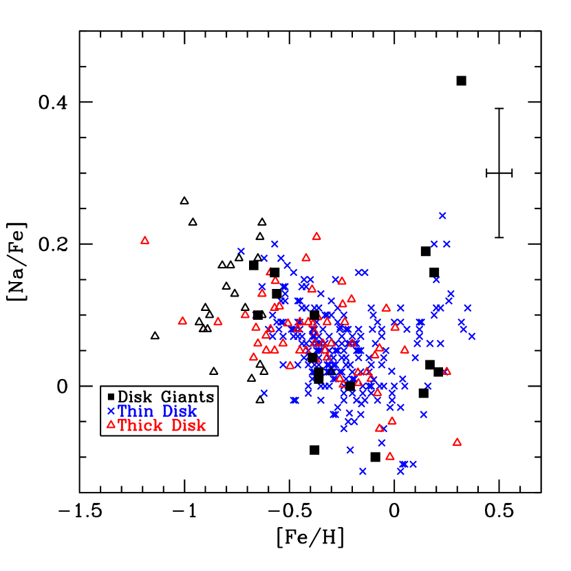
Figure 5.— Similar to Figure 4, but for [Na/Fe]. Again, $\mu$ Leo shows enhanced [Na/Fe], but the rest of the sample shows good agreement with the literature sample.

Figure 6.— Similar to Figure 4, but for [Mg/Fe]. A few of the most metal-rich disk giants show lower [Mg/Fe] ratios as compared to the comparison sample. It is unknown whether this is indicative of the true nature of the stars or the result of some flaw in our analysis. One of the metal-rich disk giants with low [Mg/Fe] is HR4450, which is most likely a binary.

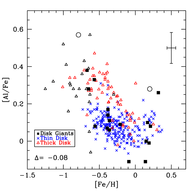
Figure 7.— Similar to Figure 4, but for [Al/Fe]. Our data points have been shifted down by 0.08 dex to adjust for possible zero-point offsets. The shift brings our metal-poor disk giants into better agreement, but it does worsen the fit for two metal-rich stars.

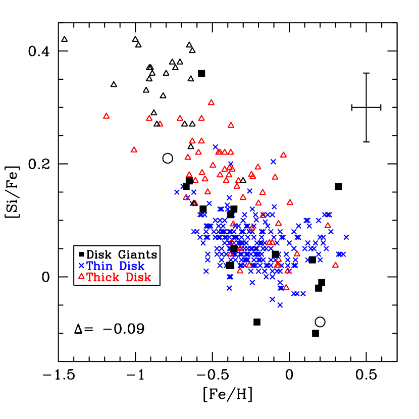
Figure 8.— Similar to Figure 4, but for [Si/Fe]. The metal-rich disk giants show a wide range of values. Like [Al/Fe], the fit to the metal-poor disk giants indicated the the need for a $-0.09$ dex shift in our zero-point to better match the literature data.

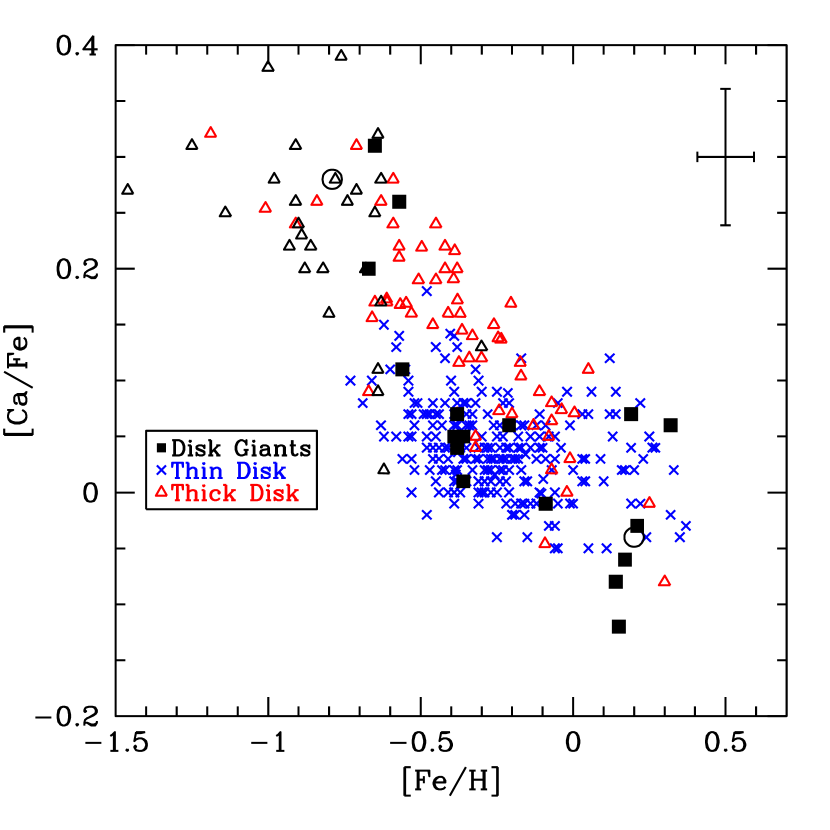
Figure 9.— Similar to Figure 4, but for [Ca/Fe]. A few of the metal-rich disk giants lie lower than similar-metallicity dwarf stars, although one of the abnormally-low disk giants is the likely binary HR4450. The metal-poor dwarfs and giants are in good agreement.

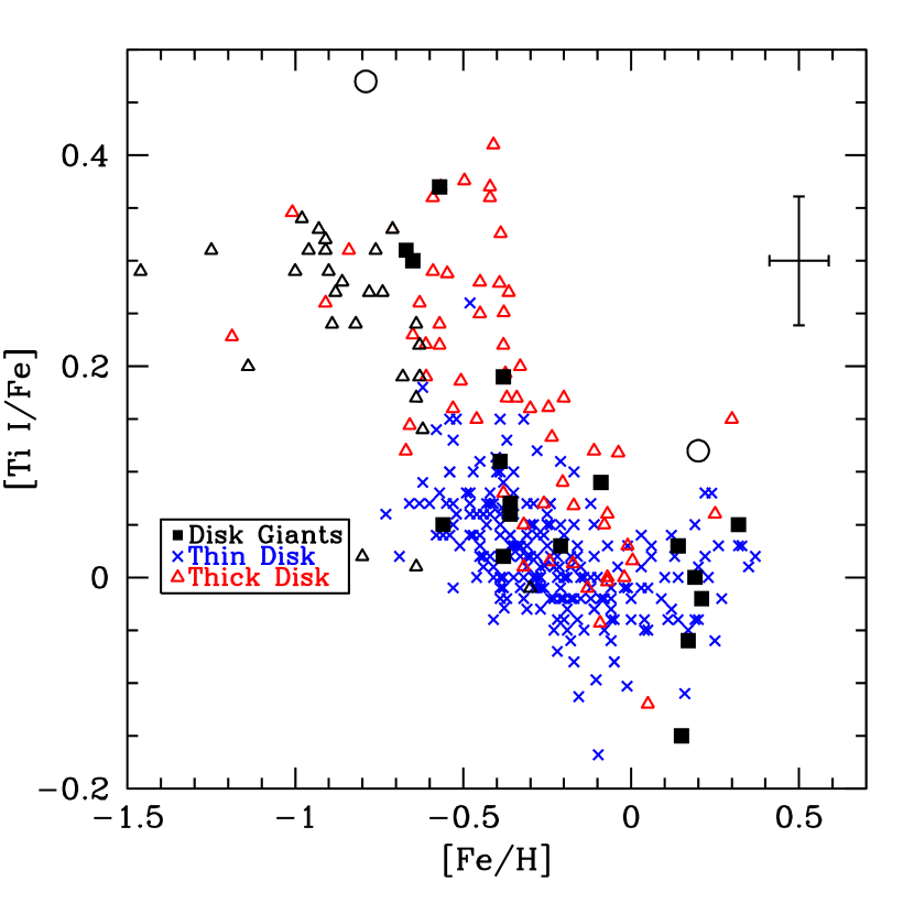
Figure 10.— Similar to Figure 4, but for [Ti/Fe]. Only the Ti I results are used for the disk giants. Again, the agreement between the dwarfs and giants is good for most of the stars.

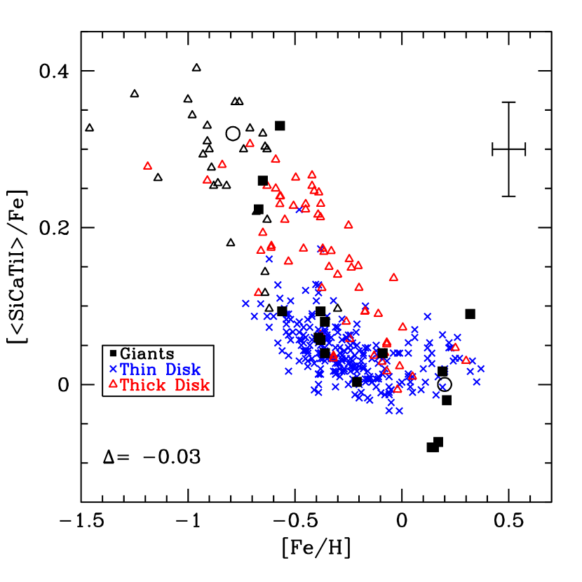
Figure 11.— [$<$SiCaTiI$>$/Fe] for our sample of disk giants (filled squares), compared to the thin disk stars (blue crosses: Reddy et al. 2003; Bensby et al. 2005; Brewer & Carney 2006), and thick disk stars (red triangles: Prochaska et al. 2000; Bensby et al. 2005; Brewer & Carney 2006; black triangles: Fulbright 2000). Due to the $-0.09$ dex shift in [Si/Fe], our data points in this plot have been shifted down by 0.03 dex.

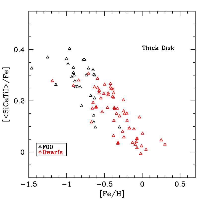
Figure 12.— A comparison of the [$<$SiCaTiI$>$/Fe] for thick disk dwarf stars (red triangles: Prochaska et al. 2000; Bensby et al. 2005; Brewer & Carney 2006) and thick disk giants from (black triangles: Fulbright 2000). The dwarf and giant data fit nicely together, without any detectable shifts.

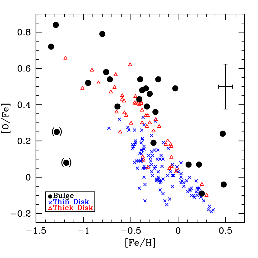
Figure 13.— The distribution of [O/Fe] vs. [Fe/H] for our bulge sample and literature values. The points are the same as in Figure 4–10. For the bulge stars, the [O/Fe] ratio drops with increasing [Fe/H], but the mean value of the distribution stays higher than the disk at the highest metallicity. The two metal-poor bulge stars with low [O/Fe] values are I-264 and IV-203 (both marked by paratheses in this and following plots). The nature of these stars are discussed in Section 9.

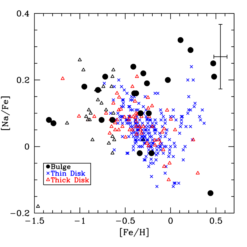
Figure 14.— Same as Figure 13, but for [Na/Fe]. The black open triangles represent thick disk stars from Fulbright (2000) using the populations identifications of Venn et al. (2004). The bulge stars show slightly-rising [Na/Fe] values with increasing [Fe/H], with [Na/Fe] near $+0.25$ for the most metal-rich stars. Two metal-poor bulge stars with high [Na/Fe] are excluded by the scale of this plot: I-264 has [Fe/H] $=-1.18$ and [Na/Fe] $=+0.57$ and IV-203 has [Fe/H] $=-1.28$ and [Na/Fe] $=+0.66$.

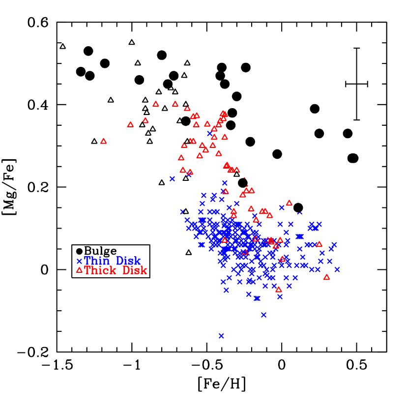
Figure 15.— Same as Figure 13, but for [Mg/Fe]. The bulge stars show enhanced [Mg/Fe] values at all metallicities, which was previously seen by MR94.

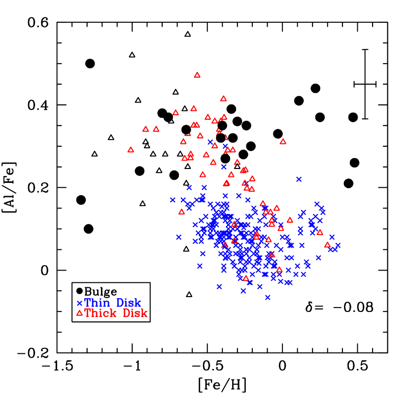
Figure 16.— A comparison of [Al/Fe] versus [Fe/H] in the Galactic bulge (filled circles), with the Galactic thin and thick disks. Like Figure 7, our data points have been shifted by $-0.08$ dex. The two stars affected by proton burning have been omitted. The bulge [Al/Fe] ratio continues to rise with [Fe/H] to at least [Fe/H]$\sim$$+$0.45 dex; whereas the thin and thick disks show declining [Al/Fe] with [Fe/H]. Notice the overlap between the thick disk and bulge around [Fe/H]$\sim$$-$0.6. There is a increase in [Al/Fe] for the bulge from $\sim$$+$0.15 dex near [Fe/H]$\sim$$-$1.3 to $\sim$$+0.40$ in the most metal-rich stars; this most likely reflects the increasing yield of Al with metallicity from Type II supernovae. The thin disk comparisons are with the data of Reddy et al. (2003, R03), Bensby et al. (2005, B05) and Brewer & Carney (2006, BC06), whilst the thick disk data points are taken from Fulbright (2000), Prochaska et al. (2000, P00), B05 and BC06.

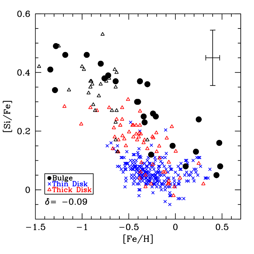
Figure 17.— Same as Figure 13, but for [Si/Fe]. Like Figure 8, our data points have been shifted by $-0.09$ dex.

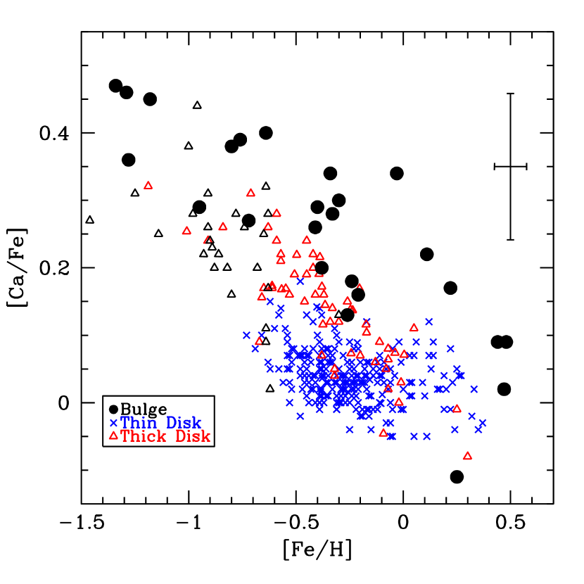
Figure 18.— Same as Figure 13, but for [Ca/Fe].

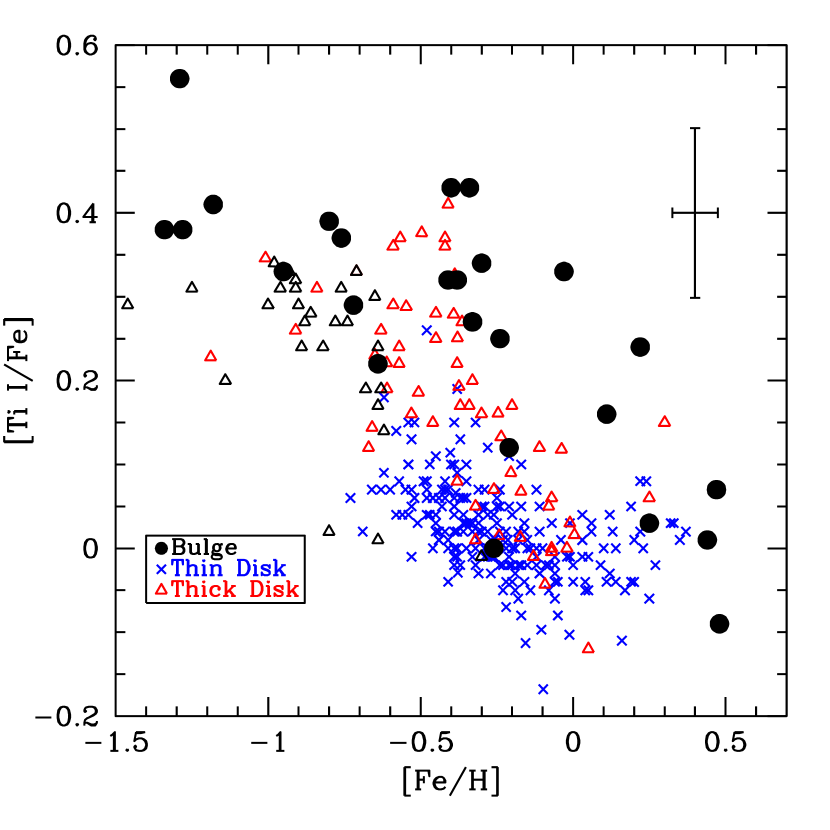
Figure 19.— Same as Figure 13, but for [Ti/Fe]. Only the Ti I results were used for this plot.

Figure 20.— A plot of [Ca/Si] and [Ca/Ti I] for our sample of bulge giants shows no obvious trend with [Fe/H], indicating that Ti and Si both track Ca. We have not applied the $-0.09$ zero-point shift to the Si abundances to the left panel. If applied, the [Ca/Si] ratio in the bulge becomes roughly solar at all metallicities.

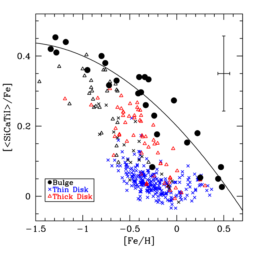
Figure 21.— [$<$SiCaTiI$>$/Fe] for our sample of bulge giants (filled circles) shifted by $-0.03$ dex (filled circles), compared to the thin disk stars (blue crosses: Reddy et al. 2003; Bensby et al. 2005; Brewer & Carney 2006), and thick disk stars (red triangles: Prochaska et al. 2000; Bensby et al. 2005; Brewer & Carney 2006; black triangles: Fulbright 2000). The bulge alpha/Fe ratios are enhanced over the thin disk by $\sim$0.2 dex. The bulge is enhanced relative to the metal-rich thick disk, by varying amounts, with the minimum difference of $\sim$0.1 dex near [Fe/H]=$-$1 dex. The solid line shows a weighted cubic polynomial fit to the bulge data, assuming no error on the [Fe/H] values; the rms scatter of the bulge points about the curve is 0.053 dex.

Figure 22.— [$<$SiCaTiI$>$/Fe] for our sample of bulge giants (filled circles), shifted by $-0.03$ dex, compared to the Galactic halo results of Fulbright (2000, plus signs) using population identifications by Venn et al (2004), and halo stars from Cayrel et al. (2004, filled squares). Note the tighter trend seen in the bulge composition; the most metal-poor bulge stars have [$<$SiCaTiI$>$/Fe] about equal to the highest seen in the halo.

Figure 23.— [O/$<$SiCaTiI$>$] and [Mg/$<$SiCaTiI$>$] for our sample of bulge giants (filled circles). The data are consistent with a linear decline in oxygen, relative to Si, Ca and Ti, over the entire [Fe/H] range; although points above solar [Fe/H] are distinctly lower than the trend at lower metallicity. The two stars whose compositions reflect proton-burning products, with O, Na and Al abundances that do not reflect the primordial composition, have been omitted for clarity. An approximately linear increase in magnesium, relative to Si, Ca and Ti, is evident over the full range of [Fe/H].

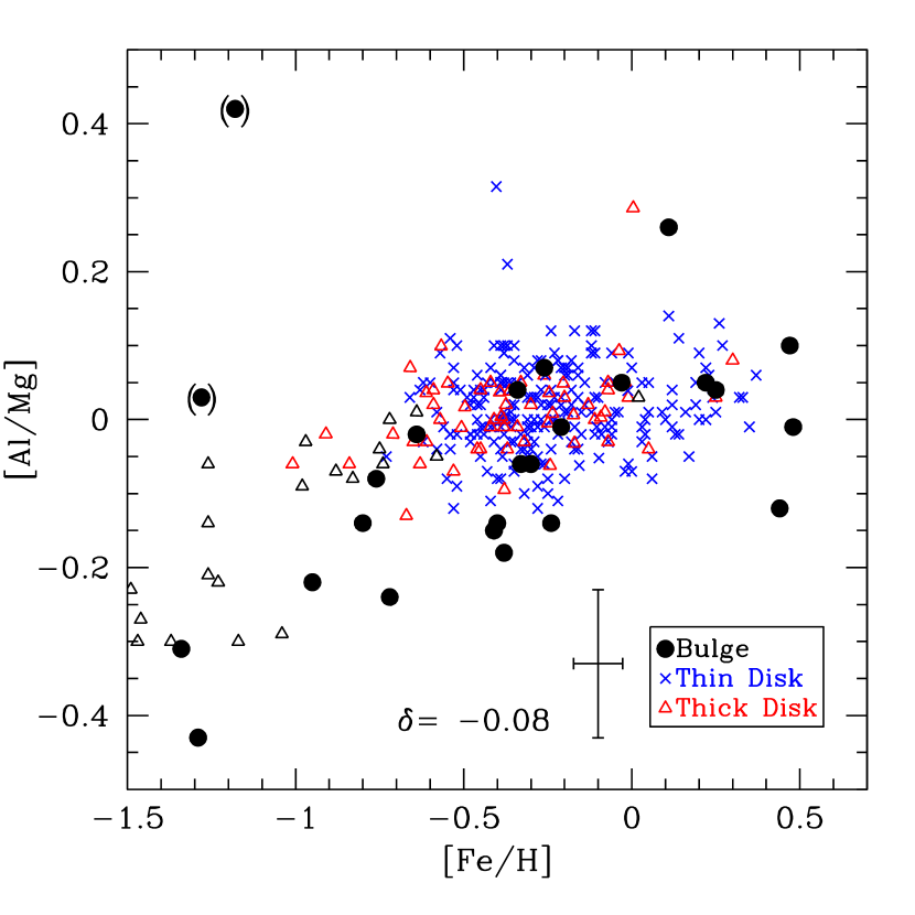
Figure 24.— A comparison showing [Al/Mg] versus [Fe/H] trends in the Galactic bulge (filled circles), thin disk (blue crosses), and thick disk (red triangles). Our data points have been shifted by $-0.08$ dex to account for possible zero-point offsets in the Al results. The trend for the three populations appears identical; thus, our bulge Al abundances corroborate our unusual Mg values. Removing the shift from our Al abundances would not affect this conclusion. Points slightly above, and separated from, the mean trend may be due to enhanced contribution from high mass Type II SNe. The two points in parentheses represent stars we have identified as being affected by envelope proton burning, with Al abundances that do not reflect their primordial compositions.

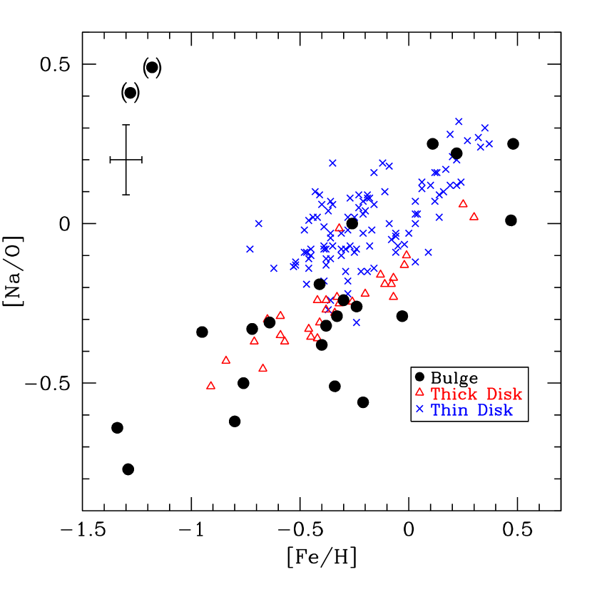
Figure 25.— A comparison showing [Na/O] versus [Fe/H] trends in the Galactic bulge (filled circles), thin disk (blue crosses), and thick disk (red triangles). The thick disk results show scatter significantly smaller than the bulge and thin disk; perhaps suggesting either larger measurement uncertainties in the bulge and thin disk, or more than one source of Na. The two points in parentheses represent stars we have identified as being affected by envelope proton burning, with Na and O abundances that do not reflect their primordial compositions.

Figure 26.— A comparison of the distinctly different [Al/Fe] versus [Fe/H] trends in the Galactic bulge (filled circles), the Galactic thin disk (crosses), and the Sagittarius dwarf spheroidal galaxy (open circles). Our data points have been shifted by $-0.08$ dex. Points in parentheses represent stars we have identified as being affected by envelope proton burning, with O and Al abundances that do not reflect their primordial compositions. Clearly, the evolution of [Al/Fe] with [Fe/H] depends upon the environmental parameters for stellar systems.

Figure 27.— The panels show the anti-correlation of Na and Al to O in the globular clusters M4 and M5 plus the four metal-poor [Fe/H] $<-1$ bulge giants in our survey. Both globular clusters have [Fe/H] values similar to the bulge stars ([Fe/H] $\sim-1.2$). The bulge stars lie very close to the locus defined by M4. Similar-metallicity field stars mostly lie in the regions denoted in the lower right corners by the dotted lines (see, for example, Figures 13, 14 and 16.

References

- Adelberger et al. (2003) Adelberger, K. L., Steidel, C. C., Shapley, A., E. & Pettini, M. 2003, ApJ, 584, 45
- Allende Prieto et al. (2001) Allende Prieto, C., Lambert, D. L. & Asplund, M., 2001, ApJ, 556, L63
- Alonso et al. (1999) Alonso, A., Arribas, S. & Martinez-Roger, C. 1999, A&AS 140, 261
- Arnett (1971) Arnett, W. D. 1971, ApJ, 166, 153
- Baade (1963) Baade, W. 1963, in Evolution of Stars and Galaxies, ed. W. Baade & C. P. Gaposhkin (Cambridge: Harvard Univ. Press), 279
- Ballero et al. (2006) Ballero, S.K., Matteucci, F., Origlia, L., & Rich, R.M. 2006, A&A, submitted.
- Barbuy et al. (2006) Barbuy, B. et al. 2006, 449, 349
- Bensby et al. (2003) Bensby T., Feltzing S. & Lundström I. 2003, A&A, 410, 527
- Bensby et al. (2005) Bensby T., Feltzing S., Lundström I. & Ilyin I. 2005, A&A, 433, 185
- Bihain et al. (2004) Bihain, G., Israelian, G., Rebolo, R., Bonifacio, P., & Molaro, P. 2004, A&A, 423, 777
- Blanco & Blanco (1984) Blanco, V. M. & Blanco, B. M. 1984, PASP, 96, 603
- Brewer & Carney (2006) Brewer, M. M., & Carney, B.W. 2006, AJ, 131, 431
- Brown, Wallerstein & Zucker (1997) Brown, J.A., Wallerstein, G. & Zucker, D. 1997, AJ, 114, 180
- Cannon et al. (1998) Cannon, R. D., Croke, B. F. W., Bell, R. A., Hesser, J. E. & Stathakis, R. A. 1998, MNRAS, 298, 601
- e.g., Carretta et al. (2001) Carretta, E., Cohen, J. G., Gratton, R. G. & Behr, B. B. 2001, AJ, 122, 1469
- Castro et al. (1996) Castro, S., Rich, R. M., McWilliam, A., Ho, L. C., Spinrad, H. & Filippenko, A. V. 1996, AJ, 111, 2439
- Cayrel et al. (2004) Cayrel, R., Depagne, E., Spite, M., Hill, V., Spite, F., et al. 2004, A&A, 416, 1117
- Combes (2001) Combes, F. 2001, in Galaxy Disks and Disk Galaxies, ASP Conf Ser Vol 320, J. Fumes and M. Corsini (eds) San Francisco: ASP p. 213
- Cunha & Smith (2006) Cunha, K. & Smith, V. V. 2006, ApJ, In Press
- Dwek et al. (1995) Dwek, E. et al. 1995, ApJ, 445, 716
- Eggen et al. (1962) Eggen, O. J., Lynden-Bell, D. & Sandage, A. R. 1962, ApJ, 136, 748
- Elmegreen (1999) Elmegreen, B. G. 1999, ApJ, 515, 323
- Ferraras et al. (2003) Ferreras, I., Wyse, R. F. G. & Silk, J. 2003, MNRAS, 345, 1381
- Figer et al. (2004) Figer, D. F., Rich, R. M., Kim, S. S., Morris, M. & Serabyn, E. 2004, ApJ, 601, 319
- Fulbright (2000) Fulbright, J. P. 2000, AJ, 120, 1841 (F00)
- Fulbright (2002) Fulbright, J. P. 2002, AJ, 123, 404
- Fulbright & Johnson (2003) Fulbright, J. P. & Johnson, J. A. 2003, ApJ, 595, 1154
- Fulbright et al. (2006a; hereafter Paper I) Fulbright, J. P., McWilliam, A. & Rich, R. M. 2006, ApJ, 636, 821
- Fulbright et al. (2006b) Fulbright, J. P., Rich, R. M. & McWilliam, A. 2006, in The Metal Rich Universe meeting proceedings, in prep.
- Gratton et al. (2004) Gratton, R. F., Sneden, C. & Carretta, E. 2003, ARA&A, 42, 385
- Gratton & Sneden (1990) Gratton, R. F. & Sneden, C. 1990, A&A, 234, 366
- Griffin (1964) Griffin, R. F. 1964, Obs, 84, 154
- Hinkle et al. (2000) Hinkle, K., Wallace, L., Valenti, J., & Harmer, D., eds. 2000, Visible and Near Infrared Atlas of the Arcturus Spectrum 3727–9300 Å (San Francisco: ASP)
- Immeli et al. (2004) Immeli, A, Samland, M., Gerhard, O., Westera, P. 2004, ApJ 611, 20
- Ivans et al. (1999) Ivans, I. I., Sneden, C., Kraft, R. P., Suntzeff, N. B., Smith, V. V., Langer, G. E. & Fulbright, J. P. 1999, AJ, 118, 1273
- Ivans et al. (2001) Ivans, I. I., Kraft, R. P., Sneden, C., Smith, G. H., Rich, R. M. & Shetrone, M. 2001, AJ, 122, 1438
- Iwamoto et al. (1999) Iwamoto, K., Brachwitz, F., Nomoto, K., Kishimoto, N., Umeda, H., Hix, W.R. & Thielemann, F.-K. 1999, ApJS, 125, 439
- Johnson et. al. (2005) Johnson, C. I., Kraft, R. P., Pilachowski, C. A., Sneden, C., Ivans, I. I. & Benman, G. 2005, PASP, 117, 1308
- Kormendy & Kennicutt (1994) Kormendy, J. & Kennicutt, R. C., Jr. 2004, ARA&A, 42, 603
- Kraft (1994) Kraft, R. P. 1994, PASP, 106, 553
- Kuijken & Rich (2002) Kuijken, K. & Rich, R. M. 2002, 124, 2054
- Kurucz et al. (1984) Kurucz, R.L., Furenlid, I., & Brault, J. 1984, in National Solar Observatory Atlas, vol. 1, Solar Flux Atlas from 296 to 1300nm (Sunspot: NSO)
- Kurucz (1993) Kurucz, R.L. 1993, IAU Commission 43, Ed. E.F.Milone, p.93
- Lambert & Ries (1981) Lambert, D.L., & Ries, L.M. 1981, ApJ, 248, 228
- Luck & Bond (1985) Luck, R.E., Bond, H.E. 1985, ApJ, 292, 559
- Lodders (2003) Lodders, K. 2003, ApJ, 591, 1220
- Mao & Paczynski (2002) Mao, S. & Paczynski, B. 2002, MNRAS, 337, 895
- Matteucci & Brocato (1990) Matteucci, F. & Brocato, E. 1990, ApJ, 365, 539
- Matteucci et al. (1999) Matteucci, F., Romano, D. & Molaro, P.
- Maeder (1980) Maeder, A. 1980, A&A, 90, 311
- Maeder (1991) Maeder, A. 1991, A&A, 242, 93
- Maeder (1992) Maeder, A. 1992, A&A, 264, 105
- McWilliam (1990) McWilliam, A. 1990, ApJS, 74, 1075
- McWilliam & Rich (1994; hereafter MR94) McWilliam, A., & Rich, R.M. 1994, ApJS, 91, 749 (MR94)
- McWilliam et al. (1995) McWilliam, A., Preston, G.W., Sneden, C., & Shectman, S. 1995a, AJ, 109, 2736
- McWilliam et al. (1995) McWilliam, A., Preston, G.W., Sneden, C., & Searle, L. 1995b, AJ, 109, 2757
- McWilliam (1997) McWilliam, A. 1997, ARA&A, 35, 503
- McWilliam & Rich (2004; hereafter MR04) McWilliam, A., & Rich, R.M. 2004, in Origin and Evolution of the Elements, ed. A. McWilliam & M. Rauch, Carnegie Observatories: Pasadena, (http://www.ociw.edu/ociw/symposia/series/symposium4/proceedings.html)
- McWilliam & Smecker-Hane (2005) McWilliam, A., & Smecker-Hane, T.A. 2005, in Cosmic Abundances as Records of Stellar Evolution and Nucleosynthesis in honor of David L. Lambert, ASP Conference Series, Vol. 336, eds. T.G.Barnes & F.N.Bash. San Francisco: Astronomical Society of the Pacific, 2005, p.221
- e.g., Meleńdez et al. (2003) Meneńdez, J. et al. 2003, A&A, 411, 417
- Meynet & Arnould (2000) Meynet, G. & Arnould, M. 2000, A&A, 355, 176
- Meynet & Maeder (2002) Meynet, G. & Maeder, A. 2002, A&A, 390, 561
- Mitchell & Mohler (1965) Mitchell, W. E., Jr. & Mohler, O. C. 1965, ApJ, 141, 1126
- Nissen & Schuster (1997) Nissen, P.E., & Schuster, W.J. 1997, A&A, 326, 751
- Origlia et al. (2005) Origlia, L., Valenti, E., Rich, M. R. & Ferraro, F. R. 2005, MNRAS, 363, 897
- Ortolani et al. (1995) Ortolani, S. et al. 1995, Nature, 377, 701
- Palacios et al. (2005) Palacios A., Arnould, M. & Meynet, G. 2005, A&A, 443, 243
- Pettini et al. (2002) Pettini, M., Rix, S.A., Steidel, C.C., Adelburger, K.L., Hunt, M.P., & Shapley, A.E. 2002, ApJ, 569, 742
- Pfenniger & Norman (1990) Pfenniger, D., & Norman, C.A. 1990, ApJ, 363, 391
- Prochaska et al. (2000) Prochaska, J.X., Naumov, S.O., Carney, B.W., McWilliam, A., & Wolfet, A.M. 2000, ApJ, 120, 2513
- Puzia et al. (2002) Puzia, T. H. 2002, A&A, 395, 45
- Ramiŕez et al. (2000) Ramiŕez, S. V., Stephens, A. W., Frogel, J. A., & DePoy, D. L. 2000, AJ, 120, 833
- Reddy et al. (2003) Reddy, B. E., Tomkin, J., Lambert, D. L. & Allende Prieto, C. 2003, MNRAS, 340, 304
- Reddy et al. (2006) Reddy, B. E., Lambert, D. L. & Allende Prieto, C. 2006, MNRAS, 367, 1329
- Renda et al. (2004) Renda, A., Fenner, Y., Gibson, B. K., Karakas, A. I., Lattanzio, J. C.; Campbell, S., Chieffi, A., Cunha, K. & Smith, V. V. 2004, MNRAS, 354, 575
- Rich (1988) Rich, R. M. 1988, AJ, 95, 828
- Rich & McWilliam (2000; hereafter RM00) Rich, R.M., & McWilliam, A. 2000, SPIE, 4005, 150 (RM00)
- Rich & Origlia (2005) Rich, R. M. & Origlia, L. 2005, ApJ, 634, 1293
- Rich et al. (2006) Rich, R.M., Fulbright, J., McWilliam, A., & Origlia, L. 2006, in Stellar Populations Cozumel meeting ASP conf series, in press
- Ruland et al. (1980) Ruland, F., Holweger, H., Griffin, R., & Biehl, D. 1980, A&AS, 42, 391
- Rutledge et al. (1997) Rutledge, G. A., Hesser, J. E. & Stetson, P. B. 1997, PASP, 109, 907
- Shetrone (1996) Shetrone, M. D. 1996, AJ, 112, 1511
- Shetrone et al. (2003) Shetrone, M. D., Venn, K.A., Tolstoy, E., Primas, F., Hill, V., & Kaufer, A. 2003, AJ, 125, 684
- Smith & Ruck (2000) Smith, G. & Ruck, M. J. 2000, A&A, 356, 570
- Sneden (1973) Sneden, C. 1973, ApJ, 184, 839
- Soto Vicencio et al. (2006) Soto Vicencio, Rich, R. M. & Kuijken, K. 2006, in preparation
- Steenbock (1975) Steenbock, W. 1985, in Cool Stars with Excesses of Heavy Elements, eds. M.Jascheck & P.C. Keenan (Dordrecht: Reidel), 231
- Steidel et al. (1996) Steidel, C. C., Giavalisco, M., Pettini, M., Dickinson, M., & Adelberger, K.L. 1996, ApJ, 462, 17
- Smecker-Hane & McWilliam (2002) Smecker-Hane, T. & McWilliam, A. 2002, astro-ph/0205411
- Sweigart & Mengel (1979) Sweigart, A.V., & Mengel, J.G. 1979, ApJ, 229, 624
- Sumi et al. (2003) Sumi, T. Eyer, L., Wozniak, P.R. 2003, MNRAS, 340, 1346
- Thielemann et al. (1996) Thielemann, F.-K., Nomoto, K. & Hashimoto, M. 1996, ApJ, 460, 408
- Thomas et al. (2003) Thomas, D., Marastron, C. and Bender, R. 2003, MNRAS, 343, 279.
- Timmes et al. (1995) Timmes, F. X., Woosley, S. E. & Weaver, T. A. 1995, ApJS, 98, 617
- Tinsley (1979) Tinsley, B. M 1979, ApJ, 229, 1046
- Venn et al. (2004) Venn, K.A., Irwin, M., Shetrone, M.D., Tout, C.A., Hill, V., & Tolstoy, E. 2004, AJ, 128, 1177
- Vogt et al. (1994) Vogt, S. S., et al. 1994, Proc. SPIE, 2198, 362
- Weaver et al. (1989) Wheeler, J. C., Sneden, C. & Truran, J. W., Jr. 1989, ARA&A, 27, 279
- Whitford (1978) Whitford, A. E. 1978, ApJ, 226, 777
- Woosley & Weaver (1995) Woosley, S.E., & Weaver, T.A. 1995, ApJS, 101, 181 (WW95)
- Worthey et al. (1992) Worthey, G., Faber, S. M. & Gonzalez, J. J. 1992, ApJ, 398, 69
- Wyse & Gilmore (1992) Wyse, R.F.G., & Gilmore, G. 1992, AJ, 104, 144
- Zhang & Liu (2005) Zhang, Y. & Liu, X.-W. 2005, ApJ, 631, 61
- Zhao et al. (1994) Zhao, H., Spergel, D. N. & Rich, R. M. 1994, AJ, 108, 2154
- Zoccali et al. (2003) Zoccali, M., et al. 2003, A&A, 399, 931