The Tully–Fisher relation for S0 galaxies

Abstract

We present a study of the local $B$- and $K_{s}$-band Tully–Fisher Relation (TFR) between absolute magnitude and maximum circular speed in S0 galaxies. To make this study, we have combined kinematic data, including a new high-quality spectral data set from the Fornax Cluster, with homogeneous photometry from the RC3 and 2MASS catalogues, to construct the largest sample of S0 galaxies ever used in a study of the TFR. Independent of environment, S0 galaxies are found to lie systematically below the TFR for nearby spirals in both optical and infrared bands. This offset can be crudely interpreted as arising from the luminosity evolution of spiral galaxies that have faded since ceasing star formation.

However, we also find a large scatter in the TFR. We show that most of this scatter is intrinsic, not due to the observational uncertainties. The presence of such a large scatter means that the population of S0 galaxies cannot have formed exclusively by the above simple fading mechanism after all transforming at a single epoch. To better understand the complexity of the transformation mechanism, we have searched for correlations between the offset from the TFR and other properties of the galaxies such as their structural properties, central velocity dispersions and ages (as estimated from line indices). For the Fornax Cluster data, the offset from the TFR correlates with the estimated age of the stars in the individual galaxies, in the sense and of the magnitude expected if S0 galaxies had passively faded since being converted from spirals. This correlation implies that a significant part of the scatter in the TFR arises from the different times at which galaxies began their transformation.

1 Introduction

The Tully–Fisher relation (TFR; Tully $\&$ Fisher 1977) is one of the most important physically-motivated correlations found in spiral galaxies. The correspondence between luminosity and maximum rotational velocity ($V_{\rm max}$) is usually interpreted as a product of the close relation between the stellar and total masses of galaxies or, in other words, as the presence of a relatively constant mass-to-light ratio in the local spiral galaxy population (e.g. Gavazzi 1993, Zwaan et al. 1995). Such a general property in spirals puts strong constraints on galaxy formation scenarios (e.g. Mao et al. 1998, van den Bosch, 2000) and cosmological models (e.g. Giovanelli et al. 1997, Sakai et al. 2000). Also, the low scatter in the TFR (only $\sim 0.35$ mag in $I$-band, according to Giovanelli et al. 1997, Sakai et al. 2000, Tully & Pierce 2000 and Verheijen 2001) permits us to use this tool as a good distance estimator (e.g. Yasuda et al. 1997).

Attempts to ascertain whether S0 galaxies follow a similar TFR have two main motivations. First, if there is a TFR of S0s, it would prove useful for estimating distances in the nearby universe, particularly in clusters where S0s are very prevalent (Dressler 1980). Second, and more related to the present study, a possible scenario where S0 galaxies are the descendants of evolved spirals at higher redshifts (Dressler 1980, Dressler et al. 1997) could leave traces of this evolution in the observed TFR of S0s. Different mechanisms have been proposed as the channels for such evolution, like small mergers (Schweizer 1986), gas stripping in later types (Gunn & Gott 1972), halo stripping (Bekki et al. 2002) and galaxy harassment (Moore et al. 1998). If this kind of picture is correct, it would be expected that S0s retain some memory of their past as spirals, in particular through their TFR, and perhaps even some clues as to which of the channels they evolved down.

Only a few studies of the TFR for S0 galaxies can be found in the literature. The first effort, made by Dressler & Sandage (1983), found no evidence for the existence of a TFR for S0 galaxies. However, the limited spatial extent of their rotation curves, the inhomogeneous photographic photometry employed and the large uncertainties in the distances to their sample made it almost certain that any correlation between luminosity and rotational velocity would be lost in the observational uncertainties.

Fifteen years later, Neistein et al. (1999) explored the existence of a TFR for S0s in the $I$-band, using a sample of 18 local S0s from the field. Although some evidence for a TFR was uncovered in this study, they also found a large scatter of $0.7$ magnitudes in the relation, suggesting the presence of more heterogeneous evolutionary histories for these galaxies when compared to spirals. Also, a systematic shift $0.5$ magnitudes was found between their galaxies and the relation for local spirals.

In two papers, Hinz et al. (2001, 2003), explored the $I$- and $H$-band TFRs for 22 S0s in the Coma Cluster and 8 S0s in the Virgo Cluster. By using cluster data, they avoided some of the errors that arise from the uncertainty in absolute distances estimation. The analysis of $I$-band data from the Coma Cluster revealed very similar results to the study by Neistein et al. (1999), implying that the larger scatter of the latter could not be attributed to distance errors or the heterogeneous nature of the data. In the $H$-band, an even larger scatter of 1.3 magnitudes was found, but with a smaller offset from the corresponding spiral galaxy TFR of only 0.2 magnitudes. Interestingly, there was no evidence for any systematic difference between the results for the Virgo and Coma Clusters, despite their differences in richness and populations, implying that these factors could not be responsible for the scatter in the TFR. Given the large scatter and small shift in the $H$-band TFR for S0s compared to spirals, it was concluded that these galaxies’ properties are not consistent with what would be expected for spiral galaxies whose star formation had been truncated; instead they suggested that other mechanisms such as minor mergers are responsible for the S0s’ TFR.

By contrast, Mathieu, Merrifield & Kuijken (2002) found in their detailed dynamical modeling of six disk-dominated field S0s that these galaxies obey a tight $I$-band TFR with a scatter of only 0.3 magnitudes, but offset from the spiral galaxy TFR by a massive 1.8 magnitudes. The authors therefore concluded that these objects were consistent with being generated by passively fading spirals that had simply stopped producing stars. This result does not appear to be consistent with the previous studies, although it should be borne in mind that the galaxies in this study were selected to be disk-dominated, so they morphologically resemble spiral galaxies more than those in other work. In addition, their field locations means that they are less likely to have had their evolution complicated by mergers. It is therefore possible that these S0s really are just passively-fading spirals where those in clusters have led more complicated lives.

As can be seen, there is no general consensus as to either the scatter or the shift in the TFR for S0 galaxies when compared to spirals, and so no agreement as to their interpretation. We therefore revisit the TFR of S0 galaxies in this paper, adding our new spectral dataset from the Fornax Cluster to the existing results from literature. In addition to the new homogeneous spectral data set, we can also take advantage of the 2MASS photometry for these galaxies (Jarrett et al. 2003), to obtain consistent infrared magnitudes and structural parameters for all the galaxies. With this more systematic study of S0s, it is to be hoped that we can avoid any past problems that may have arisen due to the heterogeneous nature of the available data, to reveal the underlying physics that dictates the TFR in S0 galaxies.

The remainder of the paper is laid out as follows. In Section 2, we describe the different samples of S0s used in this study, and the data that we have adopted. Section 3 presents the main results and then discusses their implications. Finally in Section 4 our conclusions are summarised.

2 The data

2.1 Kinematics

To build the TFR of local S0 galaxies, we have collated the data on their kinematics from four previous studies. These works are: Neistein et al. (1999), hereafter N99; Hinz et al. (2001, 2003), hereafter H01 and H03, respectively; and Mathieu, Merrifield & Kuijken (2002), hereafter M02. From the sample of N99, we exclude the galaxy NGC 4649 as it has a low degree of rotational support and it presents evidence of interaction with a neighbouring system. From H01, the Sab spiral galaxy IC 4088 was also excluded. To these data, we have added the observations that we have recently obtained using the VLT of S0 galaxies in the Fornax Cluster (Bedregal, Aragón-Salamanca & Merrifield 2006, hereafter Paper I); of the galaxies observed in this cluster, seven are rotationally supported systems, so are suitable for this study. This combined data set provides us with 60 S0 galaxies with measured kinematics, the largest sample yet used in a study of the S0 TFR. The collated kinematic data values for the maximum rotation speed, $V_{\rm max}$ (for all the sample), and the central velocity dispersion, $\sigma_{0}$ (for 51 galaxies of the sample), are listed in Table A1.

2.2 Photometry

In the present study, we have adopted $K_{s}$-band photometry from the Two Micron All Sky Survey (2MASS, Jarrett et al. 2003) and $B$-band photometry from the Third Reference Catalogue of Bright Galaxies (RC3, de Vaucouleurs et al. 1991). Of the complete sample of 60 galaxies, photometry in $K_{s}$-band is available for all objects, while 54 galaxies have photometry in $B$-band.

In order to convert these data to absolute magnitudes, we need distances to all objects in the sample. In the clusters, we adopted distance moduli of 31.35 for members of the Fornax Cluster (Madore et al. 1999), a redshift of 0.0036 for the Virgo Cluster members (Ebeling et al. 1998), and a redshift of 0.0227 for Coma Cluster galaxies (Smith et al. 2004). For the field galaxies from N99, the distance moduli of Tonry et al. (2001) were used. Finally, for the M02 sample, redshifts from the NASA/IPAC Extragalactic Database were used where available. For two of their galaxies (NGC 1611 and NGC 2612), an estimate of the distance was calculated by the authors, using the systemic velocity derived from their spectra. A Hubble constant of $70\,$km s${}^{-1}\,$Mpc^-1 was adopted in converting redshifts into distances. Galactic extinction corrections were calculated using the Schlegel, Finkeiner & Davis (1998) reddening curve description, $A_{b}^{\rm\lambda}=R_{\rm\lambda}E(B-V)$, where $R_{\rm\lambda}$=4.32 and 0.37 for $\lambda=B$ and $K_{s}$, respectively. In the $B$-band, we applied the $k$-correction from Poggianti et al. (1997); no correction was applied for the $K_{s}$-band, as it is negligible. No internal extinction correction was applied to the apparent magnitudes; there is no definitive study on the internal extinction of S0 galaxies, but the apparent lack of dust in these systems suggests that such a correction would be very small. The resulting absolute magnitudes in $K_{s}$ and $B$-bands are listed in Tables A1 and A2, respectively.

In addition to the absolute magnitudes, we derived structural parameters from the spatially-extended photometry available for these galaxies. The data used were the publicly-available “postage stamp” images in the $K_{s}$-band from 2MASS. Bulge-plus-disk models were fitted directly to these images using GIM2D (Simard et al. 2002), with a Sérsic law adopted for the bulge distribution, and an exponential for the disk. In this way, we derived values for the bulge effective radius, $R_{e}$, its Sérsic index, $n$, the disk scalelength, $R_{d}$, the half-light radius, $R_{\rm half}$, the bulge-to-total fraction, $B/T$, and the galaxy inclination $i$. In a few cases, the derived bulge scale length was found to be smaller than the seeing ($\sim 2.5$ arcsec). In those cases, the structural parameters are not well constrained by the observations, so the values were excluded. The structural parameters derived for the remaining 48 galaxies are listed in Table A1.

2.3 Line indices, ages and metallicities

We have full spectral data for 7 Fornax Cluster galaxies from which we can extract Lick indices. A detailed description of the line indices calculation is given in our forthcoming study of the stellar populations of these galaxies (Bedregal et al. 2007, hereafter Paper III). Briefly, we convolved the spectral bins with appropriate gaussians (including galactic and instrumental dispersions) in order to achieve the $3\,\rm\AA$ resolution of Bruzual & Charlot (2003) (hereafter BC03) simple stellar populations models. The indices $H\beta$, $Mgb$, $Fe\lambda 5270$ and $Fe\lambda 5335$ were measured within $R_{e}$/8 (“Central” values), between 0.75 and 1.25 $R_{e}$ (“$1\,R_{e}$” values) and between 1.5 and 2.5 $R_{e}$ (“$2\,R_{e}$” values).The resulting values are presented in Tables A2 and A3.

Central line indices for a handful of objects in our sample can be found in the literature (Fisher et al. 1996, Terlevich et al. 2002, Denicolo et al. 2004) mainly corresponding to field S0s from the N99 subsample. Unfortunately, these datasets mainly include the brightest objects of the sample, so it is difficult to make meaningful comparisons with the fainter galaxies from Fornax. Also, differences between the two samples could arise because of the superior quality of Fornax data, effect which is difficult to quantify. In consequence, we will focus our analysis of the line indices, ages and metallicities on the data from the Fornax Cluster only.

From Fornax galaxies’ indices, one can derive measures of the luminosity-weighted ages and metallicities. To this end, we have used the simple single-age stellar population models of BC03 to translate the measured line indices into estimates of age and metallicity. As a check on the uncertainties inherent in this process, we have repeated the calculations using the $Mgb$ index and the combined indices $\langle Fe\rangle$ (Gorgas, Efstathiou & Aragón-Salamanca 1990) and $[MgFe]^{\prime}$ (González 1993; Thomas, Maraston & Bender 2003) as the metallicity-sensitive index. Solar abundance ratios were assumed for the models. The resulting ages, metallicities and their uncertainties (which include the effects of covariance between the two parameters) are also shown in Tables A2 and A3.

3 Results and Discussion

The basic result of this analysis is presented in the Tully–Fisher plots of rotation velocity versus absolute magnitude shown in Figures 1 and 2 (for the $B$- and $K_{s}$-band respectively). In these plots, the solid line represents the TFR of spirals in local clusters found by Tully & Pierce (2000, hereafter TP00), shifted by $-0.207$ magnitudes in order to be consistent with the adopted Hubble constant of $H_{0}=70\,$km s${}^{-1}\,$Mpc^-1. The long-dashed line in the $B$-band represents the TFR of cluster spirals by Sakai et al. (2000, hereafter Sak00). The difference between these lines give an indication of the remaining systematic uncertainty in the spiral galaxy TFR with which we seek to compare the S0s.

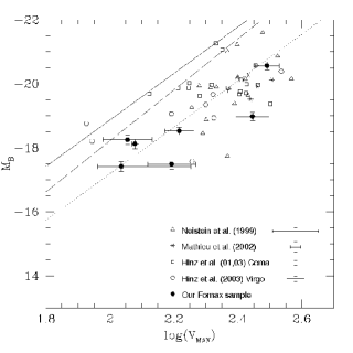
Figure 1: $B$-band Tully–Fisher relation of S0 galaxies. Solid line represents the TFR of spiral galaxies from Tully & Pierce (2000); dashed line represents the spiral TFR by Sakai et al. (2000); dotted line is the best fit to the S0 data-points using the slope from Tully & Pierce (2000). The error bars in the right down corner correspond to the median value for each subsample, while for the Fornax Cluster data we plot the errors for each data-point.

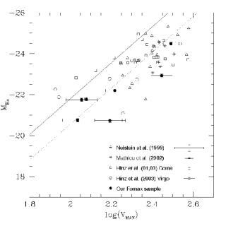
Figure 2: $K_{s}$-band Tully–Fisher relation of S0 galaxies. Solid line represents the TFR of spiral galaxies from Tully & Pierce (2000); dotted line is the best fit to the S0 data-points using the slope from Tully & Pierce (2000).The error bars in the right down corner correspond to the median value for each subsample, while for the Fornax Cluster data we plot the errors for each data-point.

3.1 Shift between the spiral and S0 TFRs

The first point that is immediately clear from Figures 1 and 2 is that, as found by previous authors, whichever spiral galaxy TFR we adopt, the S0s lie systematically below it. It is also interesting to note that this result holds true for the S0 data from all environments, from the poorest field objects to fairly rich clusters, so it is clearly a very general phenomenon. We therefore now seek to quantify and model the possible origins of such an offset.

3.1.1 Observational results

One problem in trying to quantify the offset in the TFR is that the incompleteness in magnitude of the data presented in Figures 1 and 2 will bias a conventional fit. We therefore adopt the approach of Willick (1994), which involves fitting the inverse function,

$$log(V_{\rm max})=a+bM_{\rm\lambda},\mbox{$\hskip 28.45274pt$ where $\lambda$ = $B$ or $K_{s}$},$$ (1)

to minimise this source of bias. The slope $b$ is fixed to match the slope for the spiral galaxy TFR, and $a$ is varied to find the least-squares fit between this function and the data, with each point $i$ weighted by

$$w_{i}=\frac{1}{\sigma_{i}^{2}},$$ (2)

where

$$\sigma_{i}^{2}=\sigma_{\rm log(Vmax),i}^{2}+b^{2}\sigma_{\rm M_{\lambda},i}^{2}+\sigma_{\rm int}^{2},$$ (3)

to account for the uncertainty in the measured maximum velocity, $\sigma_{\rm log(Vmax),i}$, and that in the absolute magnitude, $\sigma_{\rm M_{\lambda},i}$. The quantity $\sigma_{\rm int}$ is set to quantify the intrinsic scatter in the relation such that the reduced $\chi^{2}$ of the fit comes out at unity; this procedure is discussed in more detail in Section 3.2.

Setting $b$ equal to the inverse of the spiral TFR slope determined by TP00, we can determine the zero-point parameter $a$ and hence the offset in magnitudes from the TP00 TFR relations in the $B$- and $K_{s}$-band. The resulting best-fit lines are shown dotted in Figures 1 and 2. The offsets from the TP00 relations are

$$\Delta M_{B,TP00}=-1.7\pm 0.4$$ (4)

and

$$\Delta M_{K_{s},TP00}=-1.2\pm 0.4,$$ (5)

where the quoted error includes the uncertainty in zero point of both the S0 and spiral TFRs. To test the robustness of this result against the uncertainty in the spiral TFR, we repeated the analysis using the Sak00 $B$-band relation to fix the slope and measured the offset from their relation. This analysis resulted in an offset of

$$\Delta M_{B,\rm Sak00}=-1.3\pm 0.1,$$ (6)

within the errors of the previous analysis but somewhat smaller. Sak00 did not publish a $K_{s}$-band TFR, but the parallel nature of the Sak00 and TP00 TFRs in Figure 1 suggest that most of the difference arose from a zero-point shift due to a different distance-scale calibration. We might therefore extrapolate from the Sak00 $B$-band results on the assumption that $\Delta M_{B,TP00}-\Delta M_{K_{s},TP00}\approx\Delta M_{B,\rm Sak00}-\Delta M_{K_{s},\rm Sak00}$, to infer a corresponding $K_{s}$-band offset of

$$\Delta M_{K_{s},\rm Sak00}=-0.8\pm 0.4.$$ (7)

These new estimates for the offset between spiral and S0 TFRs tend to lie toward the upper end of earlier estimates, mainly because of the more recent refinements in the calibration to the spiral galaxy TFR that we have included in this analysis. However, even neglecting these systematic changes, the values obtained here lie within the range of offsets in the TFR suggested by previous studies, implying that this quantity can be fairly reliably determined, particularly with the larger and more homogeneous data set presented here.

3.1.2 Interpretation

The most natural interpretation of the offset between the S0 and spiral TFRs is that it represents a simple fading as a spiral galaxy’s star formation is truncated when it mutates into an S0. One complication in attempting to quantify this scenario is that one needs to know what luminosity the spiral galaxy started at in this evolution. However, observations out to redshifts beyond unity seem to show that there has been essentially no evolution in either the slope or zero-point of the spiral galaxy TFR in optical or infrared wavebands over this period (Vogt et al. 1997, Conselice et al. 2005, Bamford et al. 2006; although see Rix et al. 1997 and Böhm et al. 2004 for alternative views). This lack of evolution means that the starting point for fading spirals is the same spiral galaxy TFR that we see today, and the offset between the nearby galaxy spiral and S0 TFRs does provide an accurate measure of the degree to which the S0 galaxies must have faded if this picture is correct.

To see if this scenario is plausible and to quantify the timescales involved, we have used the BC03 synthesis models to calculate the fading of a stellar population that started with a constant star formation rate of $1\,M_{\odot}$yr^-1 for 5 Gyrs, then stopped. The stellar population was assumed to have solar metallicity and the initial mass function of Chabrier (2003). By matching the decrease in luminosity to the observed shifts between spiral and S0 TFRs, we can determine how long ago the truncation in star formation must have occurred to be consistent with our observations. Using the TP00 offsets in the $B$- and $K_{s}$-bands given in equations 4 and 5, we thus obtain times since truncation of

$$\tau_{\rm B,TP00}^{\rm trunc}=1.6^{+1.2}_{-0.7}\mbox{Gyrs}$$ (8)

and

$$\tau_{\rm K_{s},TP00}^{\rm trunc}=6.2^{+\infty}_{-3.1}\mbox{Gyrs,}$$ (9)

respectively. These values are somewhat inconsistent with each other, but this may just reflect the calibration of the spiral TFR in TP00; if we instead use the values that we infer from the Sak00 calibration (equations 6 and 7), we obtain more consistent timescales since truncation of

$$\tau_{\rm B,Sak00}^{\rm trunc}=0.66^{+0.63}_{-0.30}\mbox{Gyrs}$$ (10)

and

$$\tau_{\rm K_{s},Sak00}^{\rm trunc}=1.1^{+1.6}_{-1.0}\mbox{Gyrs}.$$ (11)

The shorter timescale simply reflects the smaller offset in the TFR that the Sak00 calibration implies. However, this timescale is if anything worryingly short: it would be quite a coincidence if we are living at an epoch so close to the point at which all these galaxies transformed from spirals into S0s.

One possible resolution is that the star formation history in transforming a spiral into an S0 might be somewhat more complex. Indeed, Poggianti et al. (1999) have suggested that cluster galaxies with k+a/a+k spectra observed at intermediate redshifts are the best candidates for S0 progenitors because of their spectro-photometric characteristics and the predominance of disk-dominated morphologies. Since such spectra are usually identified with post-starburst galaxies, it would seem that spiral galaxies may undergo a “last gasp” burst of star formation when they start their transitions into S0s. To investigate this possibility, we added a burst of star formation, amounting to 10% of the total stellar mass, to the above truncated star formation model. Repeating the comparison between the luminosity of this model as predicted by the BC03 population synthesis code and the observed offsets in the TFR resulted in estimates for the time since the burst and truncation of

$$\tau_{\rm B,TP00}^{\rm burst}=2.3^{+1.3}_{-0.8}\mbox{Gyrs},$$ (12)

$$\tau_{\rm K_{s},TP00}^{\rm burst}=7.8^{+\infty}_{-3.7}\mbox{Gyrs}$$ (13)

using the TP00 calibration, and

$$\tau_{\rm B,Sak00}^{\rm burst}=1.1^{+0.7}_{-0.4}\mbox{Gyrs,}$$ (14)

$$\tau_{\rm K_{s},Sak00}^{\rm burst}=1.7^{+1.9}_{-1.1}\mbox{Gyrs}$$ (15)

using the Sak00 values. As might be expected, the inclusion of a starburst increases the age of the stellar population compared to those found in the truncation model. These values are therefore a little more comfortable in terms of the timescales involved, and, at least using the Sak00 calibration, produce fairly consistent results between different wavebands.

However, there is a limit to how far it is worth pursuing these simple models, as it is extremely unlikely that all S0 galaxies will have undergone the same star formation history. Indeed, the large scatter apparent in the points in Figures 1 and 2 indicates a relatively heterogeneous history for these systems: the average evolution may be as described above, but each galaxy has its own story to tell. We therefore now look in more detail at the scatter in the S0 TFR, in an attempt to quantify it and explore its origins.

3.2 The Scatter in TFR of S0 galaxies

3.2.1 Observational results

As outlined in the previous section, we estimate the intrinsic scatter in the TFR, $\sigma_{\rm int}$, during the fitting process by varying its value in the weights of equation 2 until the reduced $\chi^{2}$ of the fit,

$$\chi_{r}^{2}=\frac{1}{n-2}\sum_{i}\Big{(}\frac{\log(V_{\rm max,i})-a-bM_{\rm\lambda,i}}{\sigma_{i}}\Big{)}^{2},$$ (16)

was equal to unity. The inverse slope of the TFR, $b$, was set to the value appropriate to either the TP00 or the Sak00 spiral TFR (the values are so similar that it made no substantial difference to the measured scatter), while the zero-point $a$ was allowed to vary. The presence of variables in both numerator and denominator of equation 16 mean that the fit is no longer linear, but we found that it could be robustly performed by a simple iterative procedure in which at the $j$th iteration the estimate for $\sigma_{\rm int}$ was updated such that

$$\sigma_{\rm int,j}^{2}=\sigma_{\rm int,j-1}^{2}\times\chi_{r}^{2\alpha}.$$ (17)

By setting the convergence parameter $\alpha$ to $2/3$, we found that the iterative solution was well behaved and converged in no more than 15 iterations. For comparison, we also calculated a weighted total scatter using the formula

$$\sigma_{\rm tot}^{2}=\frac{\sum_{i}w_{i}(\log(V_{max,i})-a-bM_{\rm\lambda,i})^{2}}{\sum_{i}w_{i}}.$$ (18)

For the $B$-band TFR of S0s (using TP00 slope), we thus derived

$$\begin{array}[]{rcl}\sigma_{\rm tot,B}&=&0.88\pm 0.06\mbox{ mag},\\ \sigma_{\rm int,B}&=&0.78\pm 0.06\mbox{ mag},\end{array}$$ (19)

while for $K_{s}$-band data (using TP00 slope) we found

$$\begin{array}[]{rcl}\sigma_{\rm tot,K_{s}}&=&0.98\pm 0.06\mbox{ mag},\\ \sigma_{\rm int,K_{s}}&=&0.87\pm 0.06\mbox{ mag}.\end{array}$$ (20)

These values imply that $\approx$ 90$\%$ of the observed scatter in Figures 1 and 2 cannot be explained by the known observational uncertainties in $M_{\rm\lambda}$ and log($V_{\rm max}$). These results seem to be bracketed by previous estimates: H03 report a scatter in the $H$-band TFR of 1.18 magnitudes in the Coma Cluster and 1.33 in the Virgo Cluster, whereas previous $I$-band estimates of scatter have been lower at 0.68 magnitudes (N99) and 0.82 magnitudes (H03). However, these previous studies are not directly comparable to the current estimates, because of their different wavebands and because they did not use the more robust inverse-fitting approach adopted here. In addition, it is not entirely clear whether the previous estimates have been corrected for measurement error, particularly in the uncertain measurement of $\log(V_{\rm max})$.

3.2.2 Interpretation

Perhaps the simplest possible explanation for the large value $\sigma_{\rm int}$ is that the errors in the observed quantities plotted in Figures 1 and 2 have been underestimated, and have been erroneously attributed to the intrinsic scatter. We therefore begin by considering possible additional sources of uncertainty in the data.

The adopted fluxes for the sample galaxies, particularly the infrared 2MASS data, form a uniformly-measured reliable set, so it is unlikely that much of the scatter in the TFR could arise from errors in these data. However, their transformation into absolute magnitudes could introduce some uncertainty. For example, we have not applied any correction to the magnitudes due to the internal extinction of these systems. Although such corrections are believed to be small in the relatively dust-free environment of an S0, they might still be non-negligible. However, if such an effect were distorting the results, we would expect it to have a much stronger effect in the $B$-band than in the $K_{s}$-band; the very similar values for $\sigma_{\rm int}$ derived in both bands imply that extinction is not a significant issue. Similarly, it is possible that unaccounted errors in the adopted distances to the sample galaxies could contribute to the scatter in absolute magnitudes. However, although such an error could offset all the points derived from S0s in a single cluster, it would not increase their scatter. The lack of offsets between the Virgo, Coma and Fornax Cluster data and their similar large scatters in Figures 1 and 2 imply that such errors are not significant.

The measurement of $\log(V_{\rm max})$ is more challenging. The measured Doppler shift in the stellar component is only indirectly related to this quantity. First, since we only measure the line-of-sight component of velocity, a correction must be applied for inclination. However, it is in the nature of identifying S0 galaxies that only those relatively close to edge-on are classified as such (Jorgensen & Franx 1994): as Table A1 confirms, the vast majority of galaxies in the sample are at inclinations close to 90 degrees, so the corrections are relatively small. Second, the stars in S0s do not follow perfectly circular orbits, so the measured rotation velocity will differ from the circular speed by a quantity termed the “asymmetric drift” (Binney & Tremaine 1987). For the Virgo, Coma and Fornax Cluster data, we have adopted the approach of N99 that uses the measured random velocities to correct for the asymmetric drift; although this relatively simple correction may contain systematic uncertainties, it is unlikely to increase the scatter significantly. It is also notable that the new Fornax Cluster kinematic data used here reach to larger radii than the earlier samples. Since the size of the asymmetric drift correction decreases with radius, we would expect any scatter induced by it to be smaller for these larger-radii data, but no differences are discernible. Finally, we note that M02 used a more sophisticated dynamical modeling technique that removed the need for any asymmetric drift correction. Although they claimed a resulting decrease in the scatter in the TFR, the better photometry presented in this paper suggests that this is only marginally the case. Irrespective of the way that $\log(V_{\rm max})$ is derived, there seems to be a sizeable residual scatter in the TFR.

We therefore now consider possible astrophysical origins for the scatter in the TFR. In this context, it is notable that the scatter that we derive, although much larger than that seen in the TFR of nearby spirals ($\sim 0.4$ magnitudes; TP00, Sak00, Verheijen 2001), is similar to the scatter observed in the TFR of galaxies at higher redshift. Bamford et al. (2006) obtained similar values for $\sigma_{\rm int}$ for their sample of high-redshift spirals in the $B$-band, while Conselice et al. (2005) found a similar scatter in their $K$-band TFR of spirals at redshifts between 0.2 and 1.2. This larger scatter in the spiral TFR at higher redshift has been attributed to variations in the star formation rate in these systems due to more frequent interactions with other galaxies, gas clouds and cluster environment, as well as the less relaxed dynamical state of these systems (e.g. Shi et al. 2006, Flores el at. 2006). It is therefore possible that the scatter in the S0 TFR was in some sense imprinted into these systems while they were still “normal” spiral galaxies at higher redshift, and that scatter has remained frozen into their TFR as they have evolved more gently to the present day. Alternatively, the scatter could be a signature of the transformation process itself. For example, if the transition from spiral to S0 began over a range of times, then different galaxies will have faded by different amounts, leading to the observed scatter in the relation. As we have seen in Section 3.1, the mean TFR will shift downward by more than a magnitude on billion-year timescales, so a spread in start times could explain the ultimate scatter. As a further complication, subsequent minor mergers might induce extra late bursts of star formation, or they could kill off the galaxy’s star formation a little sooner, further scattering the relation. In order to try to distinguish between these possibilities, we now investigate whether the offset of individual S0s from the spiral galaxy TFR correlates with any of their other astrophysical properties.

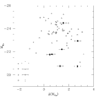
Figure 3: Plot of infrared absolute magnitude, $M_{\rm K_{s}}$, against offset from the TFR, vs $\Delta M_{\rm K_{s}}$. In the lower left corner, the median uncertainties for the N99, M02, H01 and H03 subsamples are shown, while errors for the individual Fornax Cluster data are shown.

3.3 Correlations with other parameters

3.3.1 Structural parameters

In searching for correlations between the offset from the infrared TFR, $\Delta M_{K_{s}}$, and other structural parameters, one concern is that the offset may not be the driving variable. In particular, residual bias in the fitting of the TFR to Figures 1 and 2 could induce a correlation between $\Delta M_{K_{s}}$ and the absolute magnitude of the galaxies, $M_{K_{s}}$. Since it is well know that other properties such as galaxies’ sizes correlate with their magnitudes, then such a bias in the TFR fit would also induce correlations with $\Delta M_{K_{s}}$. In practice, Figure 3 shows that there is only the slightest hint of an anti-correlation between the derived values $\Delta M_{K_{s}}$ and $M_{K_{s}}$, so this potential source of bias has clearly been dealt with reasonably effectively.

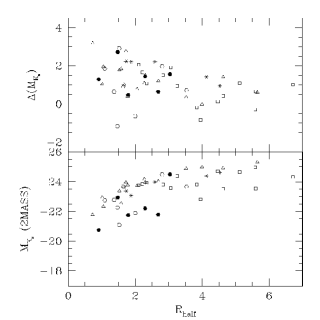
Figure 4: $M_{\rm K_{s}}$ and $\Delta M_{\rm K_{s}}$ versus half-light radius.

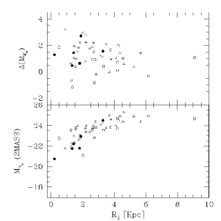
Figure 5: $M_{\rm K_{s}}$ and $\Delta M_{\rm K_{s}}$ versus disk scalelength.

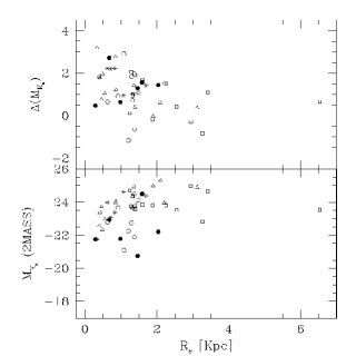
Figure 6: $M_{\rm K_{s}}$ and $\Delta M_{\rm K_{s}}$ versus bulge effective radius.

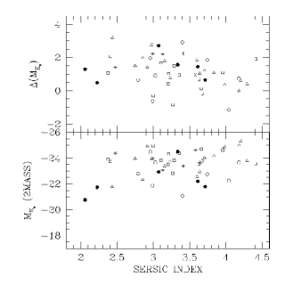
Figure 7: $M_{\rm K_{s}}$ and $\Delta M_{\rm K_{s}}$ versus Sérsic Index of the bulge.

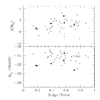
Figure 8: $M_{\rm K_{s}}$ and $\Delta M_{\rm K_{s}}$ versus bulge-to-total luminosity ratio.

Figures 4 – 9 show the correlations between the various structural properties of the S0 galaxies (as presented in Table A1 in the appendices), and their absolute magnitudes and offset from the spiral galaxy TFR in $K_{s}$-band. The symbols used in these figures are the same as in Figures 1 and 2. Some of the resulting correlations are fairly trivial. For example, the absolute magnitude correlates quite well with the size of the galaxy, as characterised by its half-light radius (see Figure 4). It is, however, interesting to note that this correlation is mainly driven by the size of the disks in these systems (see Figure 5), and is almost uncorrelated with the photometric properties of the bulge (see Figures 6 and 7). Similarly, as Figure 8 shows, the magnitudes do not seem to be systematically affected by how much of the total luminosity is in the bulge or disk components. However, we also notice that cluster galaxies are mainly responsible of the scatter in Figures 4 and 6, while field S0s tend to follow tighter trends in both diagram. However, such a difference between cluster and field galaxies could be related to different selection criteria, so any further interpretation would be excessive.

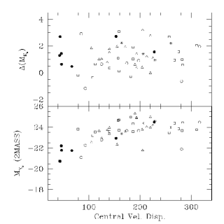
Figure 9: $M_{\rm K_{s}}$ and $\Delta M_{\rm K_{s}}$ versus central velocity dispersion.

The lack of correlation with bulge photometric properties make it intriguing that the absolute magnitude does correlate with the central velocity dispersion, which is primarily a property of the galaxy’s bulge (see Figure 9). Presumably, this correlation is a manifestation of the well-known conspiracy by which rotation curves remain fairly flat across regions dominated by bulge, disk or halo: this conspiracy means that the bulge dispersion will be tightly related to the rotation speed in the disk, and, as we have seen above, disk properties do correlate with total luminosity.

In our attempt to understand the origins of the offset from the spiral galaxy TFR, it is the correlation of parameters with this offset, $\Delta M_{K_{s}}$, that is of more immediate interest. For most plots, however, there are no significant correlations to be seen; where there is some hint of a correlation, it goes in the opposite sense to that seen with $M_{K_{s}}$, suggesting that it may well be the kind of artifact discussed at the beginning of this section.

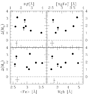
Figure 10: $\Delta M_{\rm B}$ versus $H\beta$, $\langle Fe\rangle$, $[MgFe]^{\prime}$ and $Mgb$ central line indices for our Fornax data. The error bar in the lower left corner of each panel shows the median error. Dots with arrows indicate upper limits in $\Delta M_{\rm B}$.

3.3.2 Spectral parameters

A further hint as to the origins of the scatter in the TFR can be found by considering line index measurements and the infered luminosity-weighted ages from stellar populations synthesis models. For the reasons outlined in Section 2, from this point we focus our analysis on our Fornax sample only.

Giving the homogeneity of the Fornax dataset, we feel confident to use the offset from the $B$-band TFR, $\Delta M_{\rm B}$, for the rest of the analysis. Despite the fact that uncertainties in RC3 $B$-band photometry are larger than in the 2MASS $K_{s}$-band counterpart, the total errors in $\Delta M_{\rm B}$ are dominated by the uncertainties of the TFR from spirals. Also, the $B$-band data is more sensitive to recent changes in the star formation history than the infrared band, being more suitable for this kind of study. In fact, similar results are found if the analysis is performed using $K_{s}$-band data.

Figure 10 shows $\Delta M_{\rm B}$ plotted against different central indices ($H\beta$, $Mgb$) and the combined indices $\langle Fe\rangle$ and $[MgFe]^{\prime}$. The only indication of a trend with the offset from the TFR comes from the $H\beta$ index, where $\Delta M_{\rm B}$ seems to get weaker as $H\beta$ increases, and stronger as $H\beta$ decreases. This correlation is interesting since it is in the sense expected if the degree of fading of S0s is driven by the timescale since the last significant star formation.

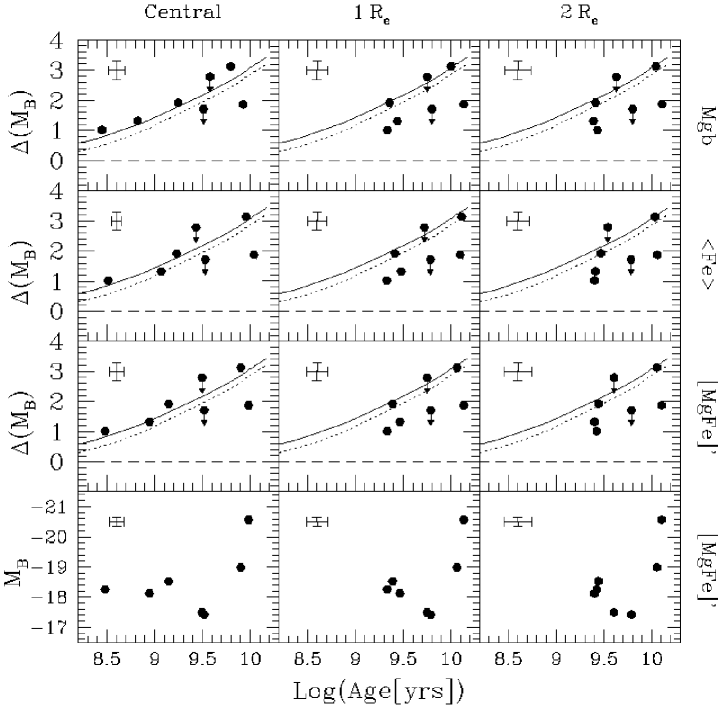
Figure 11: $\Delta M_{\rm B}$ and $M_{\rm B}$ versus ages in the center, at $1\,R_{e}$ and at $2\,R_{e}$ of the bulge, using different metallicity indicators ($Mgb$, $\langle Fe\rangle$ and $[MgFe]^{\prime}$). BC03 predictions of fading vs. age are plotted for the “truncation” (solid line) and “starburst” (dotted line) models described in section 3.1.2. Dashed horizontal lines represent the $B$-band TFR of spirals from Tully & Pierce (2000). The error bar in the upper left corner of each panel shows the median error. Dots with arrows indicate upper limits in $\Delta M_{\rm B}$. For ESO 358$-$G059 (dot with arrow of smaller shift) we re-plot the results at $1\,R_{e}$ in the column corresponding to $2\,R_{e}$.

This possibility can be examined more quantitatively if we use the age we derived from these spectral indices in Section 2. To ascertain whether the resulting ages have being significantly influenced by enhancement of $\alpha$-elements via the well-known age-metallicity degeneracy, we consider the estimates derived using $Mgb$, $\langle Fe\rangle$ and $[MgFe]^{\prime}$ parameters as the metallicity-sensitive index; the results are shown in Figure 11. The first column of this figure confirms the trend indicated by the central line indices alone: the fading of the Fornax Cluster S0s seems to be accompanied by an ageing of their stellar population. Suggestively, the size of the effect is also of the amplitude expected for a passively fading stellar population: as we saw in Section 3.1.2, over $\sim 1.6\,{\rm Gyr}$, we would expect a stellar population to fade by $\sim 1.7$ magnitudes in the $B$-band, just as seen with these data. The predictions from these models are overplotted in all the pertinent panels of Figure 11. The second and third columns of this figure present similar data at $1\,R_{e}$ and $2\,R_{e}$. The correlations are stronger for central values than at larger galactocentric distances: a Spearman ranking correlation coefficient test shows that the correlation between central age and $\Delta M_{\rm B}$ is significant at between the 90% to 97.5% level, while at larger radii the confidence level decreases to a range between 85% to 90% level only. Apart from the obvious increment in age uncertainties with S/N ratio (so with radius), there is another plausible explanation for the apparent radial dependence of the relation. If high redshift spirals simply swith-off their star formation in order to become local S0s, the age versus $\Delta M_{\rm B}$ relation would be sensitive to the relative differences in luminosity-weighted age at the moment the passive fading starts. The importance of these differences will depend, among other factors, on the relative SFRs of the progenitor spirals and their radial SFR profile before truncation. This would introduce additional scatter to the discussed result. However, there is a possible mechanism which would diminish this effect in the inner regions: a central starburst. If a central starburst precedes the truncation of the star formation, the central ages would be “set to zero” just before passive fading starts. In consequence, relative differences in central age are minimised and the age versus $\Delta M_{\rm B}$ relation becomes tighter. A central starburst has been proposed in the past as a possible (even as a necessary) step in the morphological transformation of a spiral into a S0 galaxy (Shioya et al. 2004, Christlein & Zabludoff 2004) and there is observational evidence in favour of this scenario (Poggianti et al. 2001; Mehlert et al. 2000, 2003; Moss & Whittle 2000). The youngest galaxies of our Fornax sample seem to have clear positive gradients in age, in agreement with this hypothesis. However, it will be in Paper III where we will be able to address this issue in detail, when we perform a detailed study of the stellar populations of these systems. Also worthy of note in Figure 11 is the absence of a similar correlation between age and $M_{B}$ at all radii. First, this lack of correlation rules out the possibility that the correlation with $\Delta M_{B}$ could be spuriously driven by a correlation with $M_{B}$, as discussed above. Second and more interestingly, it implies that there is no compelling evidence for the “downsizing” scenario (Gavazzi 1993, Boselli et al. 2001, Scodeggio et al. 2002) in S0s, which would predict that the faintest galaxies should have the youngest stellar populations.
Although suggestive, these results are not yet definitive. The significance level of the age versus $\Delta M_{B}$ relation is not strong enough to totally discard the null hypothesis, and in case of a positive correlation, many questions remain open: does this relation depends on local environment; do all S0s follow this trend or other properties, like luminosity, must be taken into account?. Clearly, what is needed is a larger set of high-quality data across a wide range of luminosities and environments to finally disentangle the life histories of these surprisingly complex objects.

4 Conclusions

This paper presents the largest compilation of data to-date in a study of the Tully–Fisher relation of nearby S0 galaxies in both $B$ and $K_{s}$-bands, using new and archival results for a sample of 60 galaxies in different environments. The principal results of this study are:

• The local TFR of S0 galaxies presents a shift with respect to the local TFR of spirals. Interpreted as a shift in luminosity, it amounts to between $-1.3\pm 0.1$ and $-1.7\pm 0.4$ in the $B$-band and between $-0.8\pm 0.4$ and $-1.2\pm 0.4$ in $K_{s}$-band, with the value depending on the calibration adopted for the spiral galaxy TFR.

• In a scenario where S0 galaxies are the descendants of spirals at higher redshifts which have simply passively faded, these offsets are consistent with a population that has been passively fading for somewhere between 1 and 6 Gyr (again depending on the adopted calibration for the spiral galaxy TFR). If we include a starburst before the truncation of the star formation, the upper end of the possible timescale since transformation increases somewhat. However, the large scatter in the TFR means that such a simple model with a single epoch of formation cannot provide the whole story.

• The total scatter in the TFR of S0s is found to be $0.88\pm 0.06$ mag in the $B$-band and $0.98\pm 0.06$ in the $K_{s}$-band. Our fitting indicates that only $\sim 10\%$ of this scatter can be attributed to the observational errors, with $\sim 90\%$ arising from the intrinsic astrophysical spread in the TFR. Such a scatter could have been “imprinted” by the larger scatter in the spiral galaxy TFR at high redshift, or it could have arisen through the subsequent somewhat stochastic evolution of these systems.

• To try to distinguish between these possibilities, we have looked for correlations between the offset from the TFR and other properties of these systems. Morphologically, a number of S0 properties correlate with their absolute magnitudes, as seen in other galaxies, but none seem to correlate strongly with the offset of this magnitude from the spiral galaxy TFR.

• By investigating line indices, we have been able to establish a reasonably strong correlation between the central ages of the Fornax Cluster galaxies’ stellar populations and their offsets from the TFR. This offset is in the sense and of the magnitude expected for a population of galaxies that transformed from spirals at various times in the past and has been passively fading ever since. A central starburst before the truncation of star formation would explain why the correlation is stronger with central age than at larger galactocentric distances.

The new data from the Fornax Cluster show that we are finally in a position to use observations of nearby S0 galaxies to obtain important archaeological clues as to the mechanisms by which these systems form. However, the relatively small number of S0s in a single cluster will always limit the significance of the resulting measurements. Clearly, we need a still-larger homogeneous dataset of the quality now attainable with telescopes like the VLT of S0 galaxies to finish off the work begun here.

Appendix A Tables

In this appendix we include tables with different parameters for each galaxy of our combined sample.

Table A1 includes a compilation of absolute magnitudes (total $K_{s}$-band from 2MASS) and shifts in magnitude from the $K_{s}$-band TFR of spiral galaxies, log($V_{max}$) and central velocity dispersions. Also, in the same table we present different structural parameters estimated using $K_{s}$-band photometry and GIM2D software (Simard et. al. 2002).

In Table A2 we present absolute magnitudes (total $B$-band from RC3) and shifts in magnitude from the $B$-band TFR of spiral galaxies, central line indices (Lick/IDS system, measured at 3$\AA$ resolution within $R_{e}/8$) and luminosity-weighted ages and metallicities for our sample of 7 S0 galaxies in Fornax cluster. Ages and metallicities were estimated using Bruzual & Charlot (2003) simple stellar population models. Similar data at $1$ and $2\,R_{e}$ of the bulge are presented in Table A3.

Table 1: Tully-Fisher and Structural Parameters of S0 galaxies.

$\#$	Name	$K_{s,tot}$	$M_{\rm K_{s}}$	$\Delta(M_{\rm K_{s}})$	$Log(V_{max})$	$\sigma_{0}$	$B/T$	$R_{\rm e}$	$R_{\rm d}$	$i$	Sérsic	$R_{\rm half}$
		[mag]	[mag]	[mag]	[$\rm km\,s^{-1}$]	[$\rm km\,s^{-1}$]		[Kpc]	[Kpc]	[o]		[Kpc]
(1)	(2)	(3)	(4)	(5)	(6)	(7)	(8)	(9)	(10)	(11)	(12)	(13)
FIELD	(N99)1
1	NGC 0584	7.30 (0.02)	-24.16 (0.10)	1.09 (0.26)	2.40 (0.09)	225 (–)a	$0.75_{\phantom{1}-0.02}^{\phantom{1}+0.06}$	$1.50_{\phantom{1}-0.04}^{\phantom{1}+0.22}$	$3.25_{\phantom{1}-0.34}^{\phantom{1}+0.34}$	$57.5_{\phantom{1}-3.7}^{\phantom{1}+4.4}$	$3.83_{\phantom{1}-0.08}^{\phantom{1}+0.18}$	2.27
2	NGC 0936	6.91 (0.02)	-24.92 (0.15)	1.42 (0.28)	2.52 (0.13)	193 (–)a	$0.38_{\phantom{1}-0.00}^{\phantom{1}+0.00}$	$1.36_{\phantom{1}-0.02}^{\phantom{1}+0.02}$	$4.36_{\phantom{1}-0.02}^{\phantom{1}+0.01}$	$33.9_{\phantom{1}-0.2}^{\phantom{1}+0.4}$	$2.92_{\phantom{1}-0.02}^{\phantom{1}+0.03}$	4.62
3	NGC 1023	6.24 (0.02)	-24.02 (0.16)	1.21 (0.29)	2.40 (0.03)	213 (–)a	$0.48_{\phantom{1}-0.00}^{\phantom{1}+0.00}$	$0.86_{\phantom{1}-0.00}^{\phantom{1}+0.01}$	$3.12_{\phantom{1}-0.02}^{\phantom{1}+0.01}$	$74.3_{\phantom{1}-0.1}^{\phantom{1}+0.1}$	$3.70_{\phantom{1}-0.02}^{\phantom{1}+0.04}$	2.69
4	NGC 1052	7.45 (0.01)	-23.78 (0.22)	0.41 (0.33)	2.28 (0.09)	204 (–)a	$0.73_{\phantom{1}-0.02}^{\phantom{1}+0.01}$	$1.39_{\phantom{1}-0.05}^{\phantom{1}+0.04}$	$1.53_{\phantom{1}-0.05}^{\phantom{1}+0.04}$	$48.2_{\phantom{1}-2.7}^{\phantom{1}+1.5}$	$4.29_{\phantom{1}-0.05}^{\phantom{1}+0.05}$	1.77
5	NGC 2549	8.05 (0.01)	-22.33 (0.23)	1.96 (0.34)	2.29 (0.07)	155 (–)a	$0.58_{\phantom{1}-0.01}^{\phantom{1}+0.01}$	$0.48_{\phantom{1}-0.01}^{\phantom{1}+0.01}$	$1.46_{\phantom{1}-0.01}^{\phantom{1}+0.02}$	$75.7_{\phantom{1}-0.3}^{\phantom{1}+0.2}$	$2.85_{\phantom{1}-0.03}^{\phantom{1}+0.02}$	1.05
6	NGC 2768	7.00 (0.03)	-24.88 (0.18)	0.35 (0.30)	2.40 (0.07)	193 (–)a	$0.52_{\phantom{1}-0.01}^{\phantom{1}+0.00}$	$3.12_{\phantom{1}-0.05}^{\phantom{1}+0.02}$	$5.23_{\phantom{1}-0.04}^{\phantom{1}+0.04}$	$70.6_{\phantom{1}-0.3}^{\phantom{1}+0.3}$	$3.98_{\phantom{1}-0.03}^{\phantom{1}+0.05}$	3.52
7	NGC 2787	7.26 (0.01)	-21.78 (0.34)	3.19 (0.41)	2.37 (0.06)	205 (–)a	$0.54_{\phantom{1}-0.08}^{\phantom{1}+0.07}$	$0.34_{\phantom{1}-0.06}^{\phantom{1}+0.05}$	$0.89_{\phantom{1}-0.07}^{\phantom{1}+0.07}$	$54.1_{\phantom{1}-2.3}^{\phantom{1}+2.4}$	$2.43_{\phantom{1}-0.31}^{\phantom{1}+0.23}$	0.72
8	NGC 3115	5.88 (0.02)	-23.95 (0.11)	2.76 (0.26)	2.57 (0.07)	220 (–)a	$0.59_{\phantom{1}-0.01}^{\phantom{1}+0.00}$	$0.84_{\phantom{1}-0.02}^{\phantom{1}+0.01}$	$2.22_{\phantom{1}-0.00}^{\phantom{1}+0.00}$	$68.2_{\phantom{1}-0.1}^{\phantom{1}+0.1}$	$2.98_{\phantom{1}-0.06}^{\phantom{1}+0.01}$	1.72
9	NGC 3384	6.75 (0.02)	-23.37 (0.15)	1.79 (0.28)	2.39 (0.06)	140 (–)a	$0.51_{\phantom{1}-0.05}^{\phantom{1}+0.04}$	$0.42_{\phantom{1}-0.07}^{\phantom{1}+0.06}$	$2.45_{\phantom{1}-0.20}^{\phantom{1}+0.13}$	$63.7_{\phantom{1}-2.1}^{\phantom{1}+1.7}$	$3.16_{\phantom{1}-0.52}^{\phantom{1}+0.48}$	1.53
10	NGC 3412	7.67 (0.01)	-22.54 (0.12)	1.84 (0.27)	2.30 (0.08)	105 (–)a	$0.43_{\phantom{1}-0.02}^{\phantom{1}+0.01}$	$0.39_{\phantom{1}-0.02}^{\phantom{1}+0.01}$	$1.72_{\phantom{1}-0.07}^{\phantom{1}+0.04}$	$62.4_{\phantom{1}-0.7}^{\phantom{1}+0.8}$	$3.60_{\phantom{1}-0.16}^{\phantom{1}+0.14}$	1.58
11	NGC 3489	7.37 (0.01)	-22.94 (0.15)	1.04 (0.28)	2.26 (0.12)	125 (–)a	$0.66_{\phantom{1}-0.02}^{\phantom{1}+0.01}$	$0.55_{\phantom{1}-0.02}^{\phantom{1}+0.02}$	$1.44_{\phantom{1}-0.04}^{\phantom{1}+0.03}$	$65.8_{\phantom{1}-0.8}^{\phantom{1}+0.6}$	$3.64_{\phantom{1}-0.10}^{\phantom{1}+0.08}$	1.01
12	NGC 4251	7.73 (0.01)	-23.65 (0.18)	1.01 (0.30)	2.33 (0.08)	120 (–)a	$0.77_{\phantom{1}-0.01}^{\phantom{1}+0.01}$	$1.34_{\phantom{1}-0.03}^{\phantom{1}+0.02}$	$1.58_{\phantom{1}-0.04}^{\phantom{1}+0.06}$	$78.1_{\phantom{1}-0.4}^{\phantom{1}+0.5}$	$3.64_{\phantom{1}-0.11}^{\phantom{1}+0.06}$	1.67
13	NGC 4382	6.14 (0.02)	-25.32 (0.14)	0.61 (0.28)	2.48 (0.06)	190 (–)a	$0.37_{\phantom{1}-0.00}^{\phantom{1}+0.00}$	$2.10_{\phantom{1}-0.01}^{\phantom{1}+0.03}$	$4.60_{\phantom{1}-0.01}^{\phantom{1}+0.01}$	$46.5_{\phantom{1}-0.1}^{\phantom{1}+0.1}$	$4.20_{\phantom{1}-0.02}^{\phantom{1}+0.01}$	5.65
14	NGC 4753	6.72 (0.02)	-24.98 (0.15)	-0.02 (0.28)	2.37 (0.04)	220 (–)a	$0.51_{\phantom{1}-0.00}^{\phantom{1}+0.01}$	$1.90_{\phantom{1}-0.01}^{\phantom{1}+0.03}$	$3.69_{\phantom{1}-0.03}^{\phantom{1}+0.03}$	$59.6_{\phantom{1}-0.2}^{\phantom{1}+0.3}$	$4.18_{\phantom{1}-0.02}^{\phantom{1}+0.04}$	4.00
15	NGC 4754	7.41 (0.03)	-23.60 (0.14)	1.93 (0.28)	2.43 (0.07)	171 (–)a	—	—	—	—	—	—
16	NGC 5866	6.87 (0.02)	-23.95 (0.10)	1.50 (0.26)	2.42 (0.04)	140 (–)a	$0.88_{\phantom{1}-0.05}^{\phantom{1}+0.01}$	$2.20_{\phantom{1}-0.28}^{\phantom{1}+0.04}$	$1.66_{\phantom{1}-0.09}^{\phantom{1}+0.22}$	$84.6_{\phantom{1}-1.3}^{\phantom{1}+0.8}$	$2.75_{\phantom{1}-0.05}^{\phantom{1}+0.02}$	2.30
17	NGC 7332	8.01 (0.01)	-23.72 (0.17)	0.77 (0.30)	2.31 (0.03)	136 (–)a	$0.39_{\phantom{1}-0.01}^{\phantom{1}+0.01}$	$0.46_{\phantom{1}-0.02}^{\phantom{1}+0.02}$	$2.16_{\phantom{1}-0.03}^{\phantom{1}+0.04}$	$77.7_{\phantom{1}-0.2}^{\phantom{1}+0.3}$	$3.23_{\phantom{1}-0.04}^{\phantom{1}+0.07}$	2.05

Notes: For all pertinent calculations, $H_{0}=70\,$km s${}^{-1}\,$Mpc${}^{-1}\,$. All structural parameters derived from $K_{s}$-band 2MASS photometry using GIM2D software (Simard et al. 2002). From (3) to (7), $1\,\sigma$ rms errors between “()”; from (8) to (12), $99\%$ confidence intervals are presented; Col (1), number of each galaxy in our combined sample; Col (2), name; Col (3), total apparent magnitude in $K_{s}$-band using 2MASS photometry; Col (4), absolute magnitude in $K_{s}$-band, using redshifts/distance modulus described in main text; Col (5), shift in $K_{s}$-band magnitude from Tully-Fisher relation of spiral galaxies from Tully & Pierce (2000); Col (6), logarithm (base 10) of the Maximum Rotational Velocity as published by the different authors of each subsample; Col (7), central velocity dispersion; Col (8), bulge to total fraction; Col (9), effective radius of the bulge component; Col (10), exponential disk scale length; Col (11), inclination angle; Col (12), Sérsic index; Col (13), half-light radius (computed by numerical integration of the best structural parameters).
(¹) Individual distance modules from Tonry et al. (2001) were used.
References: (^a) Neistein et al. (1999); (^b) Hinz et al. (2001); (^c) Bernardi et al. (2002); (^d) Our own data; (^e) Prugniel & Simien (1995), unpublished measurements from OHP; (^f) di Nella et al. (1995).

$\#$	Name	$K_{s,tot}$	$M_{\rm K_{s}}$	$\Delta(M_{\rm K_{s}})$	$Log(V_{max})$	$\sigma_{0}$	$B/T$	$R_{\rm e}$	$R_{\rm d}$	$i$	Sérsic	$R_{\rm half}$
		[mag]	[mag]	[mag]	[$\rm km\,s^{-1}$]	[$\rm km\,s^{-1}$]		[Kpc]	[Kpc]	[o]		[Kpc]
(1)	(2)	(3)	(4)	(5)	(6)	(7)	(8)	(9)	(10)	(11)	(12)	(13)
COMA2
18	DOI 215	11.12 (0.04)	-23.83 (0.05)	1.58 (0.24)	2.42 (0.05)	275.4 ( – )b	—	—	—	—	—	—
19	IC 3943	11.27 (0.04)	-23.68 (0.05)	1.00 (0.24)	2.33 (0.03)	281.8 ( – )b	—	—	—	—	—	—
20	IC 3990	10.50 (0.03)	-24.44 (0.04)	0.58 (0.24)	2.37 (0.04)	282.9 ( – )b	—	—	—	—	—	—
21	NGC 4787	11.40 (0.06)	-23.55 (0.06)	0.66 (0.25)	2.28 (0.03)	112.2 ( – )b	$0.91_{\phantom{1}-0.07}^{\phantom{1}+0.05}$	$6.53_{\phantom{1}-1.06}^{\phantom{1}+2.13}$	$1.26_{\phantom{1}-0.40}^{\phantom{1}+0.65}$	$64.7_{\phantom{1}-5.1}^{\phantom{1}+5.1}$	$3.62_{\phantom{1}-0.16}^{\phantom{1}+0.24}$	5.60
22	NGC 4892	10.63 (0.03)	-24.32 (0.04)	1.02 (0.24)	2.41 (0.01)	186.1 ( – )b	$0.14_{\phantom{1}-0.03}^{\phantom{1}+0.05}$	$1.33_{\phantom{1}-0.37}^{\phantom{1}+0.65}$	$4.56_{\phantom{1}-0.22}^{\phantom{1}+0.19}$	$77.4_{\phantom{1}-0.8}^{\phantom{1}+0.7}$	$3.21_{\phantom{1}-0.45}^{\phantom{1}+0.09}$	6.71
23	NGC 4931	10.31 (0.02)	-24.64 (0.04)	1.09 (0.24)	2.46 (0.02)	157.3 ( – )b	$0.78_{\phantom{1}-0.16}^{\phantom{1}+0.04}$	$3.41_{\phantom{1}-1.31}^{\phantom{1}+0.29}$	$9.08_{\phantom{1}-2.79}^{\phantom{1}+1.66}$	$47.0_{\phantom{1}-8.6}^{\phantom{1}+13.5}$	$3.96_{\phantom{1}-0.60}^{\phantom{1}+0.24}$	5.12
24	NGC 4934	11.15 (0.04)	-23.80 (0.05)	-0.19 (0.24)	2.21 (0.03)	79.2 ( – )b	$0.35_{\phantom{1}-0.06}^{\phantom{1}+0.05}$	$1.88_{\phantom{1}-0.40}^{\phantom{1}+0.34}$	$2.86_{\phantom{1}-0.14}^{\phantom{1}+0.13}$	$81.7_{\phantom{1}-0.8}^{\phantom{1}+0.8}$	$3.67_{\phantom{1}-0.32}^{\phantom{1}+0.30}$	3.84
25	NGC 4944	10.00 (0.03)	-24.95 (0.04)	-0.30 (0.24)	2.33 (0.02)	182.1 ( – )b	$0.57_{\phantom{1}-0.07}^{\phantom{1}+0.08}$	$2.95_{\phantom{1}-0.40}^{\phantom{1}+0.49}$	$6.17_{\phantom{1}-0.49}^{\phantom{1}+0.38}$	$75.9_{\phantom{1}-1.8}^{\phantom{1}+1.5}$	$3.00_{\phantom{1}-0.06}^{\phantom{1}+0.05}$	5.59
26	NGC 4966	10.25 (0.03)	-24.70 (0.04)	0.12 (0.24)	2.35 (0.04)	159.0 ( – )b	$0.39_{\phantom{1}-0.04}^{\phantom{1}+0.02}$	$1.25_{\phantom{1}-0.23}^{\phantom{1}+0.17}$	$4.20_{\phantom{1}-0.25}^{\phantom{1}+0.15}$	$58.4_{\phantom{1}-1.9}^{\phantom{1}+1.4}$	$3.66_{\phantom{1}-0.18}^{\phantom{1}+0.10}$	4.47
27	ZW 160$-$034	11.76 (0.05)	-23.18 (0.06)	-0.36 (0.25)	2.12 (0.04)	107.2 ( – )b	—	—	—	—	—	—
28	ZW 160$-$083	11.40 (0.05)	-23.55 (0.06)	0.35 (0.25)	2.25 (0.06)	140.2 ( – )b	—	—	—	—	—	—
29	ZW 160$-$101	11.20 (0.04)	-23.75 (0.05)	2.06 (0.24)	2.46 (0.02)	310.6 ( – )b	$0.68_{\phantom{1}-0.04}^{\phantom{1}+0.05}$	$1.29_{\phantom{1}-0.09}^{\phantom{1}+0.15}$	$3.46_{\phantom{1}-0.52}^{\phantom{1}+0.43}$	$80.2_{\phantom{1}-2.2}^{\phantom{1}+1.8}$	$2.41_{\phantom{1}-0.21}^{\phantom{1}+0.26}$	2.11
30	ZW 160$-$107	10.59 (0.03)	-24.36 (0.04)	0.94 (0.24)	2.40 (0.01)	267.2 ( – )b	$0.41_{\phantom{1}-0.02}^{\phantom{1}+0.02}$	$1.33_{\phantom{1}-0.13}^{\phantom{1}+0.12}$	$2.82_{\phantom{1}-0.10}^{\phantom{1}+0.09}$	$81.1_{\phantom{1}-0.6}^{\phantom{1}+0.4}$	$3.35_{\phantom{1}-0.32}^{\phantom{1}+0.19}$	3.26
31	ZW 160$-$109	11.13 (0.05)	-23.82 (0.06)	1.50 (0.25)	2.41 (0.09)	– ( – )	$0.75_{\phantom{1}-0.20}^{\phantom{1}+0.10}$	$2.26_{\phantom{1}-0.80}^{\phantom{1}+0.38}$	$2.67_{\phantom{1}-0.46}^{\phantom{1}+0.35}$	$47.9_{\phantom{1}-10.1}^{\phantom{1}+7.9}$	$3.28_{\phantom{1}-0.19}^{\phantom{1}+0.38}$	2.84
32	ZW 160$-$119	11.38 (0.04)	-23.57 (0.05)	0.96 (0.24)	2.32 (0.04)	– ( – )	—	—	—	—	—	—
33	ZW 160$-$214	11.04 (0.04)	-23.91 (0.05)	1.07 (0.24)	2.37 (0.06)	– ( – )	$0.71_{\phantom{1}-0.08}^{\phantom{1}+0.07}$	$1.49_{\phantom{1}-0.21}^{\phantom{1}+0.19}$	$4.07_{\phantom{1}-0.72}^{\phantom{1}+0.34}$	$72.4_{\phantom{1}-3.9}^{\phantom{1}+3.2}$	$2.38_{\phantom{1}-0.23}^{\phantom{1}+0.28}$	2.34
34	IC 3946	11.12 (0.04)	-23.83 (0.05)	1.66 (0.24)	2.43 (0.03)	– ( – )	$0.79_{\phantom{1}-0.09}^{\phantom{1}+0.08}$	$1.59_{\phantom{1}-0.25}^{\phantom{1}+0.36}$	$3.78_{\phantom{1}-0.72}^{\phantom{1}+0.30}$	$76.9_{\phantom{1}-5.1}^{\phantom{1}+3.8}$	$3.11_{\phantom{1}-0.24}^{\phantom{1}+0.31}$	2.21
35	IC 3955	11.38 (0.05)	-23.57 (0.06)	1.91 (0.25)	2.43 (0.07)	186.0 ( 9.0)c	$0.46_{\phantom{1}-0.13}^{\phantom{1}+0.10}$	$1.40_{\phantom{1}-0.62}^{\phantom{1}+0.48}$	$2.64_{\phantom{1}-0.22}^{\phantom{1}+0.32}$	$61.4_{\phantom{1}-5.2}^{\phantom{1}+4.4}$	$4.41_{\phantom{1}-0.61}^{\phantom{1}+1.04}$	3.07
36	IC 3976	11.50 (0.04)	-23.45 (0.05)	2.69 (0.24)	2.50 (0.04)	257.0 ( 6.0)c	—	—	—	—	—	—
37	IC 4111	12.13 (0.09)	-22.82 (0.10)	-0.84 (0.26)	2.03 (0.04)	– ( – )	$0.57_{\phantom{1}-0.13}^{\phantom{1}+0.10}$	$3.26_{\phantom{1}-0.60}^{\phantom{1}+0.53}$	$2.75_{\phantom{1}-0.40}^{\phantom{1}+0.50}$	$76.2_{\phantom{1}-4.3}^{\phantom{1}+4.4}$	$3.27_{\phantom{1}-0.63}^{\phantom{1}+0.39}$	3.95
38	NGC 4873	11.25 (0.04)	-23.70 (0.06)	3.08 (0.25)	2.57 (0.06)	159.0 (11.0)c	—	—	—	—	—	—
39	UGC 8122	11.45 (0.06)	-23.50 (0.07)	0.42 (0.25)	2.25 (0.15)	– ( – )	$0.34_{\phantom{1}-0.11}^{\phantom{1}+0.11}$	$2.55_{\phantom{1}-0.56}^{\phantom{1}+0.34}$	$3.32_{\phantom{1}-0.41}^{\phantom{1}+0.41}$	$51.5_{\phantom{1}-7.9}^{\phantom{1}+4.6}$	$3.20_{\phantom{1}-0.47}^{\phantom{1}+0.72}$	4.63

(²) Redshift of 0.0227 for Coma cluster assumed (Smith et al. 2004)

$\#$	Name	$K_{s,tot}$	$M_{\rm K_{s}}$	$\Delta(M_{\rm K_{s}})$	$Log(V_{max})$	$\sigma_{0}$	$B/T$	$R_{\rm e}$	$R_{\rm d}$	$i$	Sérsic	$R_{\rm half}$
		[mag]	[mag]	[mag]	[$\rm km\,s^{-1}$]	[$\rm km\,s^{-1}$]		[Kpc]	[Kpc]	[o]		[Kpc]
(1)	(2)	(3)	(4)	(5)	(6)	(7)	(8)	(9)	(10)	(11)	(12)	(13)
FORNAX3
40	NGC 1380	6.87 (0.02)	-24.49 (0.07)	1.56 (0.25)	2.49 (0.04)	227.8 ( 1.8)d	$0.58_{\phantom{1}-0.01}^{\phantom{1}+0.01}$	$1.59_{\phantom{1}-0.03}^{\phantom{1}+0.03}$	$3.28_{\phantom{1}-0.04}^{\phantom{1}+0.09}$	$66.9_{\phantom{1}-0.4}^{\phantom{1}+0.6}$	$3.34_{\phantom{1}-0.03}^{\phantom{1}+0.03}$	3.04
41	NGC 1381	8.42 (0.02)	-22.93 (0.07)	2.72 (0.25)	2.44 (0.05)	153.1 ( 1.8)d	$0.57_{\phantom{1}-0.01}^{\phantom{1}+0.01}$	$0.67_{\phantom{1}-0.01}^{\phantom{1}+0.02}$	$1.88_{\phantom{1}-0.05}^{\phantom{1}+0.07}$	$82.5_{\phantom{1}-0.3}^{\phantom{1}+0.4}$	$3.07_{\phantom{1}-0.10}^{\phantom{1}+0.14}$	1.48
42	NGC 1380A	9.57 (0.04)	-21.78 (0.08)	0.64 (0.25)	2.08 (0.01)	46.8 ( 0.9)d	$0.18_{\phantom{1}-0.03}^{\phantom{1}+0.06}$	$0.98_{\phantom{1}-0.25}^{\phantom{1}+0.32}$	$1.80_{\phantom{1}-0.06}^{\phantom{1}+0.04}$	$78.1_{\phantom{1}-0.8}^{\phantom{1}+0.6}$	$3.71_{\phantom{1}-0.10}^{\phantom{1}+0.07}$	2.69
43	NGC 1375	9.61 (0.03)	-21.75 (0.08)	0.47 (0.25)	2.06 (0.08)	66.8 ( 1.3)d	$0.19_{\phantom{1}-0.02}^{\phantom{1}+0.01}$	$0.29_{\phantom{1}-0.03}^{\phantom{1}+0.02}$	$1.33_{\phantom{1}-0.07}^{\phantom{1}+0.04}$	$67.5_{\phantom{1}-1.2}^{\phantom{1}+0.8}$	$2.22_{\phantom{1}-0.08}^{\phantom{1}+0.07}$	1.79
44	IC 1963	9.15 (0.02)	-22.20 (0.07)	1.44 (0.25)	2.22 (0.04)	46.3 ( 1.4)d	$0.39_{\phantom{1}-0.03}^{\phantom{1}+0.03}$	$2.04_{\phantom{1}-0.12}^{\phantom{1}+0.21}$	$1.42_{\phantom{1}-0.02}^{\phantom{1}+0.03}$	$84.6_{\phantom{1}-0.2}^{\phantom{1}+0.2}$	$3.61_{\phantom{1}-0.09}^{\phantom{1}+0.10}$	2.29
45	ESO 358$-$G006	10.62 (0.05)	-20.73 (0.09)	2.70 (0.26)	2.19 (0.07)	43.9 ( 0.9)d	—	—	—	—	—	—
46	ESO 358$-$G059	10.60 (0.04)	-20.75 (0.08)	1.30 (0.25)	2.04 (0.22)	42.9 ( 1.0)d	$0.72_{\phantom{1}-0.07}^{\phantom{1}+0.04}$	$1.46_{\phantom{1}-0.14}^{\phantom{1}+0.20}$	$0.21_{\phantom{1}-0.02}^{\phantom{1}+0.01}$	$61.9_{\phantom{1}-2.0}^{\phantom{1}+2.0}$	$2.06_{\phantom{1}-0.40}^{\phantom{1}+0.17}$	0.91
VIRGO4
47	NGC 4352	9.87 (0.04)	-21.08 (0.04)	2.91 (0.24)	2.26 (0.03)	85.0 ( 8.0)c	$0.76_{\phantom{1}-0.09}^{\phantom{1}+0.07}$	$1.08_{\phantom{1}-0.17}^{\phantom{1}+0.13}$	$2.02_{\phantom{1}-0.30}^{\phantom{1}+0.23}$	$80.1_{\phantom{1}-5.4}^{\phantom{1}+3.4}$	$3.40_{\phantom{1}-0.20}^{\phantom{1}+0.24}$	1.52
48	NGC 4417	8.17 (0.03)	-22.78 (0.03)	0.65 (0.24)	2.19 (0.05)	125.0 ( 4.0)c	$0.56_{\phantom{1}-0.02}^{\phantom{1}+0.02}$	$0.62_{\phantom{1}-0.02}^{\phantom{1}+0.03}$	$1.82_{\phantom{1}-0.05}^{\phantom{1}+0.04}$	$78.2_{\phantom{1}-0.4}^{\phantom{1}+0.4}$	$2.79_{\phantom{1}-0.06}^{\phantom{1}+0.07}$	1.37
49	NGC 4435	7.30 (0.02)	-23.66 (0.01)	0.72 (0.24)	2.30 (0.03)	174.0 (16.0)c	$0.53_{\phantom{1}-0.04}^{\phantom{1}+0.10}$	$1.32_{\phantom{1}-0.15}^{\phantom{1}+0.19}$	$4.20_{\phantom{1}-0.13}^{\phantom{1}+0.00}$	$15.9_{\phantom{1}-11.1}^{\phantom{1}+33.3}$	$4.18_{\phantom{1}-0.44}^{\phantom{1}+0.17}$	3.53
50	NGC 4442	7.29 (0.02)	-23.66 (0.02)	0.91 (0.24)	2.32 (0.02)	197.0 (15.0)c	$0.67_{\phantom{1}-0.01}^{\phantom{1}+0.02}$	$0.92_{\phantom{1}-0.02}^{\phantom{1}+0.04}$	$2.62_{\phantom{1}-0.05}^{\phantom{1}+0.06}$	$73.5_{\phantom{1}-0.5}^{\phantom{1}+0.8}$	$3.03_{\phantom{1}-0.03}^{\phantom{1}+0.06}$	1.63
51	NGC 4452	9.07 (0.03)	-21.88 (0.03)	-0.63 (0.24)	1.94 (0.02)	281.0 (15.0)e	$0.21_{\phantom{1}-0.07}^{\phantom{1}+0.04}$	$1.37_{\phantom{1}-0.40}^{\phantom{1}+0.24}$	$1.27_{\phantom{1}-0.03}^{\phantom{1}+0.02}$	$85.2_{\phantom{1}-0.3}^{\phantom{1}+0.2}$	$2.99_{\phantom{1}-0.10}^{\phantom{1}+0.11}$	2.00
52	NGC 4474	8.70 (0.02)	-22.26 (0.02)	-1.16 (0.24)	1.93 (0.04)	93.0 ( 7.0)c	$0.79_{\phantom{1}-0.01}^{\phantom{1}+0.02}$	$1.21_{\phantom{1}-0.07}^{\phantom{1}+0.07}$	$1.34_{\phantom{1}-0.05}^{\phantom{1}+0.09}$	$81.2_{\phantom{1}-0.6}^{\phantom{1}+1.0}$	$4.04_{\phantom{1}-0.41}^{\phantom{1}+0.26}$	1.47
53	NGC 4526	6.47 (0.02)	-24.48 (0.02)	1.96 (0.24)	2.54 (0.01)	316.0 ( 7.0)c	$0.61_{\phantom{1}-0.01}^{\phantom{1}+0.01}$	$1.37_{\phantom{1}-0.02}^{\phantom{1}+0.02}$	$4.25_{\phantom{1}-0.02}^{\phantom{1}+0.04}$	$75.9_{\phantom{1}-0.3}^{\phantom{1}+0.3}$	$2.96_{\phantom{1}-0.04}^{\phantom{1}+0.05}$	2.80
54	NGC 4638	8.21 (0.02)	-22.74 (0.02)	1.85 (0.24)	2.32 (0.02)	– ( – )	$0.74_{\phantom{1}-0.03}^{\phantom{1}+0.01}$	$1.29_{\phantom{1}-0.22}^{\phantom{1}+0.08}$	$0.50_{\phantom{1}-0.01}^{\phantom{1}+0.04}$	$79.1_{\phantom{1}-0.5}^{\phantom{1}+0.6}$	$3.74_{\phantom{1}-0.10}^{\phantom{1}+0.15}$	1.09
FIELD	(M02)5
55	NGC 1184	8.12 (0.02)	-24.59 (0.02)	0.95 (0.24)	2.43 (0.03)	229.0 (14.0)f	$0.31_{\phantom{1}-0.01}^{\phantom{1}+0.01}$	$1.07_{\phantom{1}-2.43}^{\phantom{1}+0.07}$	$3.80_{\phantom{1}-0.05}^{\phantom{1}+0.06}$	$80.8_{\phantom{1}-0.2}^{\phantom{1}+0.2}$	$3.58_{\phantom{1}-0.05}^{\phantom{1}+0.07}$	4.53
56	NGC 1611	9.41 (0.01)	-24.53 (0.01)	1.01 (0.24)	2.43 (0.02)	– ( – )	—	—	—	—	—	—
57	NGC 2612	8.78 (0.02)	-23.06 (0.02)	2.20 (0.24)	2.40 (0.02)	– ( – )	$0.44_{\phantom{1}-0.01}^{\phantom{1}+0.01}$	$0.71_{\phantom{1}-2.40}^{\phantom{1}+0.02}$	$1.83_{\phantom{1}-0.06}^{\phantom{1}+0.07}$	$75.0_{\phantom{1}-0.6}^{\phantom{1}+0.8}$	$3.13_{\phantom{1}-0.06}^{\phantom{1}+0.04}$	1.88
58	NGC 3986	8.98 (0.02)	-24.37 (0.02)	1.41 (0.24)	2.46 (0.01)	206.0 (22.0)f	$0.53_{\phantom{1}-0.01}^{\phantom{1}+0.02}$	$1.70_{\phantom{1}-2.46}^{\phantom{1}+0.09}$	$5.67_{\phantom{1}-0.11}^{\phantom{1}+0.15}$	$84.0_{\phantom{1}-0.2}^{\phantom{1}+0.3}$	$2.48_{\phantom{1}-0.06}^{\phantom{1}+0.09}$	4.13
59	NGC 4179	7.92 (0.02)	-23.36 (0.04)	2.24 (0.24)	2.44 (0.01)	164.0 (15.0)c	$0.59_{\phantom{1}-0.01}^{\phantom{1}+0.01}$	$0.83_{\phantom{1}-2.44}^{\phantom{1}+0.02}$	$2.20_{\phantom{1}-0.04}^{\phantom{1}+0.05}$	$80.5_{\phantom{1}-0.2}^{\phantom{1}+0.3}$	$3.41_{\phantom{1}-0.07}^{\phantom{1}+0.06}$	1.73
60	NGC 5308	8.36 (0.03)	-23.97 (0.05)	2.22 (0.24)	2.51 (0.02)	260.0 (12.0)f	$0.39_{\phantom{1}-0.01}^{\phantom{1}+0.04}$	$0.62_{\phantom{1}-2.51}^{\phantom{1}+0.11}$	$2.68_{\phantom{1}-0.05}^{\phantom{1}+0.12}$	$81.6_{\phantom{1}-0.2}^{\phantom{1}+0.5}$	$2.99_{\phantom{1}-0.06}^{\phantom{1}+0.04}$	2.59

(³) Distance modulus of 31.35 mag for Fornax cluster assumed (Madore et al. 1999). (⁴) Individual redshifts were used from RC3. (⁵) Individual redshidts were used from NASA/IPAC Extragalactic Database (NED); for NGC 1611 and NGC 2612, redshifts were estimated from spectra by M02.

Table 2: Central Line Indices, Ages, Metallicities and $\Delta(M_{\rm B})$ of S0 galaxies in Fornax.

Name	$M_{\rm B}$	$\Delta(M_{\rm B})$	$H\beta$	$Mgb$	$\langle Fe\rangle$	$[MgFe]^{\prime}$	$Age_{Mgb}$	$[Fe/H]_{Mgb}$	$Age_{\langle Fe\rangle}$	$[Fe/H]_{\langle Fe\rangle}$	$Age_{[MgFe]^{\prime}}$	$[Fe/H]_{[MgFe]^{\prime}}$
	[mag]	[mag]	[Å]	[Å]	[Å]	[Å]	[Gyrs]	[dex]	[Gyrs]	[dex]	[Gyrs]	[dex]
(1)	(2)	(3)	(4)	(5)	(6)	(7)	(8)	(9)	(10)	(11)	(12)	(13)
CENTRAL
NGC 1380	-20.57 (0.12)	1.87 (0.27)	1.48 (0.04)	4.92 (0.04)	3.54 (0.03)	4.15 (0.05)	$8.4_{\phantom{1}-0.9}^{\phantom{1}+1.0}$	$0.70_{\phantom{1}-0.06}^{\phantom{1}+0.07}$	$10.9_{\phantom{1}-1.3}^{\phantom{1}+1.4}$	$0.37_{\phantom{1}-0.04}^{\phantom{1}+0.04}$	$9.6_{\phantom{1}-1.4}^{\phantom{1}+1.5}$	$0.49_{\phantom{1}-0.06}^{\phantom{1}+0.06}$
NGC 1381	-18.98 (0.12)	3.13 (0.27)	1.66 (0.04)	4.43 (0.04)	3.10 (0.03)	3.72 (0.05)	$6.2_{\phantom{1}-1.0}^{\phantom{1}+1.1}$	$0.56_{\phantom{1}-0.08}^{\phantom{1}+0.08}$	$9.0_{\phantom{1}-0.9}^{\phantom{1}+1.1}$	$0.16_{\phantom{1}-0.04}^{\phantom{1}+0.04}$	$7.9_{\phantom{1}-0.8}^{\phantom{1}+1.0}$	$0.32_{\phantom{1}-0.06}^{\phantom{1}+0.06}$
NGC 1380A	-18.12 (0.15)	1.32 (0.28)	2.91 (0.08)	3.34 (0.08)	2.99 (0.07)	3.18 (0.09)	$0.7_{\phantom{1}-0.1}^{\phantom{1}+0.2}$	$1.35_{\phantom{1}-0.19}^{\phantom{1}+0.20}$	$1.2_{\phantom{1}-0.1}^{\phantom{1}+0.1}$	$0.65_{\phantom{1}-0.06}^{\phantom{1}+0.06}$	$0.9_{\phantom{1}-0.2}^{\phantom{1}+0.2}$	$0.96_{\phantom{1}-0.13}^{\phantom{1}+0.13}$
NGC 1375	-18.25 (0.15)	1.02 (0.28)	3.90 (0.09)	2.44 (0.08)	3.07 (0.06)	2.72 (0.09)	$0.3_{\phantom{1}-0.1}^{\phantom{1}+0.1}$	$1.46_{\phantom{1}-0.20}^{\phantom{1}+0.21}$	$0.3_{\phantom{1}-0.05}^{\phantom{1}+0.05}$	$1.00_{\phantom{1}-0.05}^{\phantom{1}+0.05}$	$0.3_{\phantom{1}-0.06}^{\phantom{1}+0.1}$	$1.24_{\phantom{1}-0.13}^{\phantom{1}+0.14}$
IC 1963	-18.53 (0.12)	1.92 (0.27)	2.45 (0.08)	3.76 (0.07)	3.32 (0.06)	3.55 (0.08)	$1.8_{\phantom{1}-0.04}^{\phantom{1}+0.1}$	$1.09_{\phantom{1}-0.14}^{\phantom{1}+0.14}$	$1.7_{\phantom{1}-0.2}^{\phantom{1}+0.2}$	$0.69_{\phantom{1}-0.05}^{\phantom{1}+0.05}$	$1.4_{\phantom{1}-0.2}^{\phantom{1}+0.2}$	$0.92_{\phantom{1}-0.11}^{\phantom{1}+0.11}$
ESO 358$-$G006	-17.49 (0.16)	2.78 (0.29)	2.35 (0.15)	2.52 (0.14)	2.62 (0.12)	2.60 (0.16)	$3.8_{\phantom{1}-1.6}^{\phantom{1}+2.1}$	$-0.25_{\phantom{1}-0.16}^{\phantom{1}+0.18}$	$2.7_{\phantom{1}-0.5}^{\phantom{1}+1.0}$	$0.10_{\phantom{1}-0.11}^{\phantom{1}+0.12}$	$3.1_{\phantom{1}-0.8}^{\phantom{1}+1.8}$	$-0.07_{\phantom{1}-0.17}^{\phantom{1}+0.18}$
ESO 358$-$G059	-17.41 (0.15)	1.71 (0.28)	2.26 (0.07)	3.03 (0.06)	2.57 (0.05)	2.82 (0.07)	$3.2_{\phantom{1}-0.5}^{\phantom{1}+0.8}$	$0.07_{\phantom{1}-0.09}^{\phantom{1}+0.10}$	$3.4_{\phantom{1}-0.5}^{\phantom{1}+0.6}$	$0.02_{\phantom{1}-0.05}^{\phantom{1}+0.05}$	$3.3_{\phantom{1}-0.5}^{\phantom{1}+0.7}$	$0.05_{\phantom{1}-0.08}^{\phantom{1}+0.08}$

Notes: From (2) to (7), $1\,\sigma$ rms errors between “()”; from (8) to (13), $99\%$ confidence intervals are presented. Col (1), name; Col (2), absolute total $B$-band magnitude from RC3 assuming distance modulus of 31.35 mag (Madore et al. 1999) for Fornax cluster; Col (3), shift in $B$-band magnitude from Tully-Fisher relation of spiral galaxies from Tully & Pierce (2000); Col (4), $H\beta$ index; Col (5), $Mgb$ index; Col (6), $\langle Fe\rangle$ combined index (Gorgas, Efstathiou & Aragón-Salamanca 1990); Col (7), $[MgFe]^{\prime}$ combined index (González 1993; Thomas, Maraston & Bender 2003); Col (8) (9), age and metallicity, estimated using Bruzual & Charlot (2003) simple stellar population models and $Mgb$ as metallicity indicator; Col (10) (11), age and metallicity, estimated using $\langle Fe\rangle$ as metallicity indicator; Col (12) (13), age and metallicity, estimated using $[MgFe]^{\prime}$ as metallicity indicator.

Table 3: Line Indices, Ages and Metallicities at $1$ and $2\,R_{e}$ of S0 galaxies in Fornax.

Name	$H\beta$	$Mgb$	$\langle Fe\rangle$	$[MgFe]^{\prime}$	$Age_{Mgb}$	$[Fe/H]_{Mgb}$	$Age_{\langle Fe\rangle}$	$[Fe/H]_{\langle Fe\rangle}$	$Age_{[MgFe]^{\prime}}$	$[Fe/H]_{[MgFe]^{\prime}}$
	[Å]	[Å]	[Å]	[Å]	[Gyrs]	[dex]	[Gyrs]	[dex]	[Gyrs]	[dex]
(1)	(2)	(3)	(4)	(5)	(6)	(7)	(8)	(9)	(10)	(11)
At $1\,R_{e}$
NGC 1380	1.61 (0.08)	3.62 (0.07)	2.86 (0.06)	3.21 (0.08)	$13.6_{\phantom{1}-3.0}^{\phantom{1}+4.7}$	$-0.13_{\phantom{1}-0.08}^{\phantom{1}+0.09}$	$12.4_{\phantom{1}-2.4}^{\phantom{1}+3.3}$	$-0.06_{\phantom{1}-0.07}^{\phantom{1}+0.07}$	$13.5_{\phantom{1}-2.9}^{\phantom{1}+4.6}$	$-0.14_{\phantom{1}-0.09}^{\phantom{1}+0.09}$
NGC 1381	1.61 (0.08)	3.98 (0.07)	2.82 (0.06)	3.36 (0.09)	$10.0_{\phantom{1}-2.1}^{\phantom{1}+3.0}$	$0.15_{\phantom{1}-0.10}^{\phantom{1}+0.11}$	$12.9_{\phantom{1}-2.7}^{\phantom{1}+4.4}$	$-0.11_{\phantom{1}-0.08}^{\phantom{1}+0.07}$	$11.5_{\phantom{1}-2.5}^{\phantom{1}+3.6}$	$0.00_{\phantom{1}-0.10}^{\phantom{1}+0.10}$
NGC 1380A	2.26 (0.11)	3.24 (0.10)	2.72 (0.08)	2.98 (0.12)	$2.7_{\phantom{1}-0.5}^{\phantom{1}+1.0}$	$0.26_{\phantom{1}-0.16}^{\phantom{1}+0.17}$	$3.0_{\phantom{1}-0.5}^{\phantom{1}+0.9}$	$0.14_{\phantom{1}-0.08}^{\phantom{1}+0.08}$	$2.9_{\phantom{1}-0.6}^{\phantom{1}+1.0}$	$0.19_{\phantom{1}-0.13}^{\phantom{1}+0.14}$
NGC 1375	2.50 (0.15)	2.94 (0.14)	2.75 (0.12)	2.86 (0.16)	$2.2_{\phantom{1}-0.2}^{\phantom{1}+0.6}$	$0.26_{\phantom{1}-0.20}^{\phantom{1}+0.22}$	$2.1_{\phantom{1}-0.1}^{\phantom{1}+0.4}$	$0.28_{\phantom{1}-0.12}^{\phantom{1}+0.13}$	$2.1_{\phantom{1}-0.1}^{\phantom{1}+0.5}$	$0.27_{\phantom{1}-0.19}^{\phantom{1}+0.20}$
IC 1963	2.18 (0.08)	3.74 (0.08)	3.19 (0.06)	3.45 (0.08)	$2.3_{\phantom{1}-0.3}^{\phantom{1}+0.5}$	$0.66_{\phantom{1}-0.14}^{\phantom{1}+0.15}$	$2.6_{\phantom{1}-0.3}^{\phantom{1}+0.4}$	$0.47_{\phantom{1}-0.06}^{\phantom{1}+0.06}$	$2.4_{\phantom{1}-0.3}^{\phantom{1}+0.5}$	$0.55_{\phantom{1}-0.11}^{\phantom{1}+0.11}$
ESO 358$-$G006	2.15 (0.15)	2.77 (0.14)	2.40 (0.12)	2.57 (0.16)	$5.6_{\phantom{1}-1.5}^{\phantom{1}+2.3}$	$-0.24_{\phantom{1}-0.15}^{\phantom{1}+0.16}$	$5.3_{\phantom{1}-1.3}^{\phantom{1}+1.9}$	$-0.15_{\phantom{1}-0.12}^{\phantom{1}+0.12}$	$5.6_{\phantom{1}-1.4}^{\phantom{1}+2.2}$	$-0.24_{\phantom{1}-0.16}^{\phantom{1}+0.17}$
ESO 358$-$G059	2.08 (0.16)	2.82 (0.14)	2.38 (0.12)	2.64 (0.17)	$6.3_{\phantom{1}-1.8}^{\phantom{1}+2.9}$	$-0.26_{\phantom{1}-0.16}^{\phantom{1}+0.17}$	$6.1_{\phantom{1}-1.6}^{\phantom{1}+2.5}$	$-0.21_{\phantom{1}-0.13}^{\phantom{1}+0.13}$	$6.1_{\phantom{1}-1.7}^{\phantom{1}+2.7}$	$-0.22_{\phantom{1}-0.16}^{\phantom{1}+0.18}$
At $2\,R_{e}$
NGC 1380	1.65 (0.10)	3.49 (0.10)	2.83 (0.08)	3.12 (0.11)	$12.8_{\phantom{1}-3.5}^{\phantom{1}+6.6}$	$-0.18_{\phantom{1}-0.11}^{\phantom{1}+0.12}$	$11.4_{\phantom{1}-2.5}^{\phantom{1}+3.0}$	$-0.07_{\phantom{1}-0.09}^{\phantom{1}+0.09}$	$12.6_{\phantom{1}-3.4}^{\phantom{1}+6.4}$	$-0.17_{\phantom{1}-0.12}^{\phantom{1}+0.12}$
NGC 1381	1.71 (0.08)	3.44 (0.08)	2.70 (0.06)	3.04 (0.09)	$11.0_{\phantom{1}-2.2}^{\phantom{1}+2.5}$	$-0.15_{\phantom{1}-0.09}^{\phantom{1}+0.10}$	$10.8_{\phantom{1}-2.1}^{\phantom{1}+3.4}$	$-0.15_{\phantom{1}-0.08}^{\phantom{1}+0.07}$	$11.3_{\phantom{1}-2.4}^{\phantom{1}+4.0}$	$-0.19_{\phantom{1}-0.10}^{\phantom{1}+0.10}$
NGC 1380A	2.34 (0.09)	3.28 (0.09)	2.91 (0.07)	3.10 (0.10)	$2.4_{\phantom{1}-0.4}^{\phantom{1}+0.5}$	$0.40_{\phantom{1}-0.15}^{\phantom{1}+0.16}$	$2.6_{\phantom{1}-0.3}^{\phantom{1}+0.3}$	$0.35_{\phantom{1}-0.07}^{\phantom{1}+0.07}$	$2.5_{\phantom{1}-0.4}^{\phantom{1}+0.4}$	$0.36_{\phantom{1}-0.12}^{\phantom{1}+0.12}$
NGC 1375	2.39 (0.16)	2.82 (0.14)	2.63 (0.12)	2.72 (0.16)	$2.7_{\phantom{1}-0.6}^{\phantom{1}+1.6}$	$0.04_{\phantom{1}-0.20}^{\phantom{1}+0.21}$	$2.5_{\phantom{1}-0.4}^{\phantom{1}+0.9}$	$0.13_{\phantom{1}-0.12}^{\phantom{1}+0.12}$	$2.6_{\phantom{1}-0.5}^{\phantom{1}+1.3}$	$0.06_{\phantom{1}-0.18}^{\phantom{1}+0.19}$
IC 1963	2.14 (0.16)	3.66 (0.14)	3.07 (0.12)	3.36 (0.16)	$2.6_{\phantom{1}-0.7}^{\phantom{1}+1.7}$	$0.53_{\phantom{1}-0.27}^{\phantom{1}+0.28}$	$2.9_{\phantom{1}-0.6}^{\phantom{1}+1.3}$	$0.37_{\phantom{1}-0.11}^{\phantom{1}+0.12}$	$2.8_{\phantom{1}-0.6}^{\phantom{1}+1.6}$	$0.44_{\phantom{1}-0.20}^{\phantom{1}+0.22}$
ESO 358$-$G006	2.30 (0.15)	2.57 (0.14)	2.42 (0.12)	2.49 (0.16)	$4.3_{\phantom{1}-1.8}^{\phantom{1}+2.1}$	$-0.25_{\phantom{1}-0.15}^{\phantom{1}+0.18}$	$3.5_{\phantom{1}-0.9}^{\phantom{1}+1.8}$	$-0.08_{\phantom{1}-0.11}^{\phantom{1}+0.11}$	$4.0_{\phantom{1}-1.6}^{\phantom{1}+2.0}$	$-0.20_{\phantom{1}-0.16}^{\phantom{1}+0.17}$
ESO 358$-$G0591	— (—)	— (—)	— (—)	— (—)	—	—	—	—	—	—

Notes: From (2) to (5), $1\,\sigma$ rms errors between “()”; from (6) to (11), $99\%$ confidence intervals are presented. Col (1), name; Col (2), $H\beta$ index; Col (3), $Mgb$ index; Col (4), $\langle Fe\rangle$ combined index (Gorgas, Efstathiou & Aragón-Salamanca 1990); Col (5), $[MgFe]^{\prime}$ combined index (González 1993; Thomas, Maraston & Bender 2003); Col (6) (7), age and metallicity, estimated using Bruzual & Charlot (2003) simple stellar population models and $Mgb$ as metallicity indicator; Col (8) (9), age and metallicity, estimated using $\langle Fe\rangle$ as metallicity indicator; Col (10) (11), age and metallicity, estimated using $[MgFe]^{\prime}$ as metallicity indicator.
(¹) For ESO 358$-$G059 no data is available at $2\,R_{e}$ of the bulge. In consequence, for this particular galaxy, we re-plot in Figure 11 the results at $1\,R_{e}$ in the column corresponding to $2\,R_{e}$.

References

- (1) Bamford S. P., Aragón-Salamanca A., Milvang-Jensen B., 2006, MNRAS, 366, 308B
- (2) Bedregal A.G., Aragón-Salamanca A., Merrifield M.R., 2006, Accepted in MNRAS (astro-ph/0607433, Paper I)
- (3) Bedregal A.G., Aragón-Salamanca A., Cardiel N., Merrifield M.R., 2007, in prep., (Paper III)
- (4) Bekki K., Shioya Y., Couch W.J, 2002, ApJ, 577, 651
- (5) Bernardi M., Alonso M.V., da Costa L.N., Willmer C.N.A., Wegner G., Pellegrini P.S., Rité C., Maia M.A.G., 2002, AJ, 123, 2990B
- (6) Binney J., Tremaine S., 1987, “Galactic Dynamics”, Princeton Series in Astrophysics
- (7) Böhm A., et al., 2004, A&A, 420, 97
- (8) Boselli A., Gavazzi G., Scodeggio, M., 2001, AJ, 121, 753
- (9) Bruzual G, Charlot S., 2003, MNRAS, 244, 1000B
- (10) Bureau M.& Chung A., 2006, MNRAS, 366, 182B
- (11) Chabrier G., 2003, PASP, 115, 763
- (12) Conselice C. J., Bundy K., Ellis R. S., Brichmann J., Vogt N. P., Phillips A. C., 2005, ApJ, 628, 160
- (13) Christlein D., Zabludoff A.I., 2004, ApJ, 616, 192
- (14) Denicoló G., Terlevich R., Terlevich E., Forbes D.A., Terlevich A., Carrasco L., 2005, MNRAS, 356, 1440D
- (15) De Vaucouleurs G., De Vaucouleurs A., Corwin JR. H.G., Buta R.J. Paturel G., Fouque P., 1991, Third Reference Catalog of Bright Galaxies.
- (16) Di Nella H., Garcia A.M., Garnier R., Paturel G., 1995, A&AS, 113, 151D
- Dressler (1980) Dressler A., 1980, ApJ, 236, 351
- (18) Dressler A., Sangade A., 1983, ApJ, 265, 664
- Dressler et al. (1997) Dressler A., et al., 1997, ApJ, 490, 577
- (20) Ebeling H., Edge A.C., Bohringer H., Allen S.W., Crawford C.S., Fabian A.C., Voges W., Huchra J.P., 1998, MNRAS, 301, 881E
- (21) Fisher D., Franx M., Illingworth G., 1996, ApJ, 459, 110F
- (22) Flores H., Hammer F., Puech M. Amram P., Balkowski C., 2006, submitted to A&A, astro-ph/0603563
- Gavazzi (1993) Gavazzi G., 1993, ApJ, 419, 469
- (24) Giovanelli R., Haynes M.P., da Costa L.N., Freudling W., Salzer J.J., Wegner G., 1997, ApJ, 477L, 1G
- (25) González J.J., 1993, PhD Thesis, University of California, Santa Cruz
- (26) Gorgas J., Efstathiou G., Aragón-Salamanca A., 1990, MNRAS, 245, 217
- (27) Gunn J.E., Gott J.R.I., 1972, ApJ, 176, 1
- (28) Hinz J.L., Rix H.-W., Bernstein G.M., 2001, AJ, 121, 683
- (29) Hinz J.L., Rieke G.H., Caldwell N., 2003, AJ, 126, 2622
- (30) Jarret T.H., Chester T., Cutri R., Schneider S.E., Huchra J.P., 2003, AJ, 125, 525J
- (31) Jorgensen I., Franx M., 1994, ApJ, 433, 553
- (32) Madore B.F., Freedman W.L., Silbermann N., et al., 1999, ApJ, 515, 29
- Mao et al. (1998) Mao S., Mo H. J., White S.D.M., 1998, MNRAS, 297, L71
- (34) Mathieu A., Merrifield M., Kuijken K., 2002, MNRAS, 330, 251
- (35) Mehlert D., Saglia R.P., Bender R., Wegner G., 2000, A&AS, 141, 449
- (36) Mehlert D., Thomas D., Saglia R.P., Bender R., Wegner G., 2003, A&A, 407, 423
- Moore et al. (1998) Moore B., Lake G., Katz N., 1998, ApJ, 495, 139
- (38) Neistein E., Maoz D., Rix H.-W., Tonry J.L., 1999, AJ, 117, 2666
- (39) Poggianti B. M., 1997, A&AS, 122, 399P
- (40) Poggianti B. M., Smail I., Dressler A., Couch W. J., Barger A. J., Butcher H., Ellis R. S., Oemler A., 1999, ApJ, 518, 576
- (41) Poggianti B., Bridges T.J., Carter D. et al. 2001, ApJ 563, 118
- (42) Prugniel Ph., Simien F., 1995, ASPC, 86, 151P
- (43) Rix H-W, Guhathakurta P., Colless M., Ing K., 1997, MNRAS, 285, 779R
- (44) Sakai S., Mould J.R., Hughes S.M.G., et al., 2000, ApJ, 529, 698
- (45) Schlegel D.J., Finkbeiner D.P., Davis M., 1998, ApJ, 500, 525S
- (46) Schweizer F., 1986, Sci, 231, 227S
- (47) Scodeggio M., Gavazzi G., Franzetti P., Boselli A., Zibetti S., Pierini D., 2002, A&A, 384, 812
- (48) Shioya Y., Bekki K., Couch W.J., 2004, ApJ, 601, 654
- (49) Shi Y., Rieke G.H., Papovich C., Pérez-González P.G., Le Floch E., 2006, Accepted in ApJ (astro-ph/0603453)
- Simard (2002) Simard L., Willmer C.N.A., Vogt N.P. et al., 2002, ApJS, 142, 1S
- (51) Smith R.J., Hudson M.J., Nelan J.E., Moore A.W., Quinney S.J., Wegner G.A., Lucey J.R., Davies R.L., Malecki J.J., Schade D., Suntzeff N.B., 2004, AJ, 128, 1558S
- (52) Terlevich A.I., Forbes D.A., 2002, MNRAS, 330, 547
- (53) Thomas D., Maraston C., Bender R., 2003, MNRAS, 339, 897
- (54) Tonry J.L., Dressler A., Blakeslee J.P., et al., 2001, ApJ, 546, 681T
- (55) Trager S.C., Faber S.M., Worthey G., González J.J., 2000a, AJ, 119, 1645
- (56) Trager S.C., Faber S.M., Worthey G., González J.J., 2000b, AJ, 120, 165
- (57) Tully R.B., Fisher J.R., 1977, A&A, 54, 661T
- (58) Tully R.B., Pierce M.J., 2000, ApJ, 533, 744
- (59) Van den Bosch F.C., 2000, ApJ, 530, 177V
- (60) Verheijen M.A.W., 2001, ApJ, 563, 694
- (61) Vogt N.P., et al., 1997, ApJ, 479, L121
- (62) Willick J.A., 1994, ApJS, 92, 1
- (63) Yasuda N., Fukugita M., Okamura S., 1997, ApJS, 108, 417Y
- (64) Zwaan M.A., van der Hulst J.M., De Blok W.J.G., McGaygh S.S., 1995, MNRAS, 273L, 35Z