The Lidar System of the
Pierre Auger Observatory

Abstract

The Pierre Auger Observatory in Malargüe, Argentina, is designed to study the origin of ultrahigh energy cosmic rays with energies above $10^{18}$ eV. The energy calibration of the detector is based on a system of four air fluorescence detectors. To obtain reliable calorimetric information from the fluorescence stations, the atmospheric conditions at the experiment’s site need to be monitored continuously during operation. One of the components of the observatory’s atmospheric monitoring system is a set of four elastic backscatter lidar stations, one station at each of the fluorescence detector sites. This paper describes the design, current status, standard operation procedure, and performance of the lidar system of the Pierre Auger Observatory.

, , , , , , , , , , , , , , , , , , , , , , , , , , , , , and

1 Introduction

The Pierre Auger Observatory in Malargüe, Argentina, the world’s largest facility to detect ultrahigh energy cosmic rays with energies above $10^{18}$ eV, is currently nearing completion. Data collection started in January 2004, and the observatory has already accumulated an ultrahigh energy cosmic ray data set of unprecedented size.

Due to their extremely low flux, primary cosmic rays at ultrahigh energies cannot be observed directly. Rather, they enter the atmosphere and interact with air molecules, inducing a cascade of secondary particles, called an extensive air shower. The properties of the primary particle (energy, arrival direction, and chemical composition) have to be deduced from indirect measurements of the extensive air shower.

Two detector types have traditionally been used to measure air showers: surface detectors, which detect the particles of the air shower cascade that reach the ground; and air fluorescence detectors, which make use of the fact that the particles in the air shower excite air molecules, causing UV fluorescence. Observing this UV light from air showers with photomultiplier cameras allows us to image the air shower development and obtain a nearly calorimetric energy estimate of the shower. For both detector types, the atmosphere acts as the calorimeter and provides the large detector volume needed to measure the small cosmic ray flux at the highest energies.

The Pierre Auger Observatory is a hybrid detector which combines a large surface detector (SD) array of area $3000\,\mathrm{km}^{2}$ and a system of four fluorescence telescopes (FD) at the same site. While the SD provides the well-defined aperture and the $100\,\%$ duty cycle needed to achieve high statistics, the FD provides, for a subset of showers, the calorimetric information needed to calibrate the SD.

For the calibration to be meaningful, the properties of the calorimeter, i.e. the atmosphere, must be well-known. Particulates in the atmosphere, Cherenkov radiation and the weather need to be factored into this calibration. Fluorescence light from air showers is affected by the absorption and scattering on molecules and aerosols, and, in addition, some fraction of the Cherenkov radiation from the relativistic particles in the air shower is scattered into the detector. This Cherenkov light cannot be separated from the fluorescence light, and so the contamination by Cherenkov light needs to be modeled and subtracted to give an accurate energy estimate for the cosmic ray shower. Moreover, the light transmission properties of the atmosphere are not constant over the large detector volume of the Pierre Auger Observatory, and equally important, they are not constant in time. Changing weather conditions inevitably mean changing transmission properties. Consequently, the properties of the atmosphere need to be monitored continuously.

The Pierre Auger Observatory has an extensive program to monitor the atmosphere within the FD aperture and measure atmospheric attenuation and scattering properties in the 300 to 400 nm sensitivity range of the FDs. A summary of the atmospheric monitoring system can be found in [1]. Within this system, a central role is played by a system of four elastic backscatter lidar (light detection and ranging) stations, one at each fluorescence site. system is currently under construction, with three out of four stations operating. At each lidar station, a high-repetition UV laser sends short laser light pulses into the atmosphere in the direction of interest. The backscattered signal is detected as a function of time by photomultiplier tubes at the foci of parabolic mirrors. Both the laser and the mirrors are mounted on a steering frame that allows the lidar to cover the full azimuth and elevation of the sky.

During each hour of FD data taking, the four lidars perform a routine scan of the sky over each FD. The data provide information about the height and coverage of clouds as well as their depth and opacity, and the local aerosol scattering and absorption properties of the atmosphere. In addition to this routine operation, the lidar system is used for real time monitoring of the atmospheric homogeneity between the FDs and selected cosmic ray events. For example, if a high energy “hybrid” event is observed with the SD and one or more FDs, the routine scan is interrupted and, within 2 to 4 minutes of the event detection, the lidar scans the atmosphere in the vicinity of the air shower reported by the FD. This procedure is called ”shoot-the-shower” (StS), and allows for a rejection of events where the light profile from the track is distorted by clouds or other aerosol non-uniformities that are not characterized well by the average hourly aerosol measurements. Both light reflection and opacity can distort the light profile.

This paper describes the design, standard operation procedure, and performance of the lidar system of the Pierre Auger Observatory. It is organized as follows. After a brief description of the SD and FD detectors (Section 2), we give a summary of the relevant atmospheric parameters (Section 3). Section 4 describes the current lidar hardware. In Section 5, the daily operating procedure is summarized, including a description of the routine scan and the shoot-the-shower operation. First results of the analysis of atmospheric parameters like cloud height and extinction are summarized in Section 6. A section on inelastic Raman lidar measurements and a summary conclude the paper.

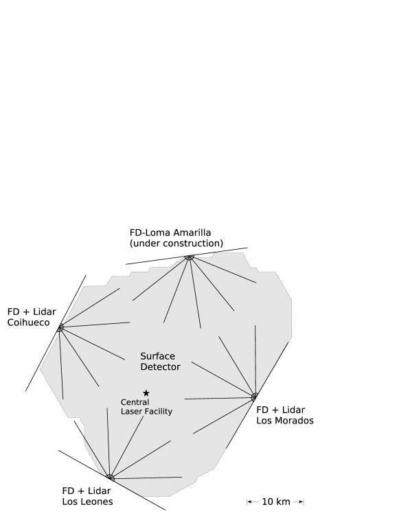
Figure 1: Schematic layout of the Pierre Auger Observatory.

2 The Pierre Auger Observatory

In its final stage, the surface detector array of the Pierre Auger Observatory will comprise 1600 water Cherenkov detector tanks, deployed over an area of $3000\,\mathrm{km}^{2}$ on a triangular grid with 1500 m grid spacing. Each of these cylindrical plastic tanks is 1.5 m tall with a $10\,\mathrm{m}^{2}$ base, and filled with 12,000 liters of purified water within a Tyvek liner. Three $9^{\prime\prime}$ photomultiplier tubes in the tanks measure the Cherenkov light produced by the particles of the extensive air shower cascade traversing the tank water.

The SD measures the particle density as a function of distance to the shower core, defined as the location where the primary particle would have hit the ground had it not showered in the atmosphere. The SD array therefore measures the lateral profile of the shower at ground level. The SD operates with a nearly $100\,\%$ duty cycle.

For a fraction of the showers, the SD measurement is complemented by a measurement of the longitudinal profile of the shower in the atmosphere. This information is provided by four fluorescence detectors. Unlike Cherenkov light, which is strongly forward-peaked, fluorescence light is emitted isotropically. The fluorescence signal from the air shower is small compared to other light sources, but during dark, moonless nights, about $10\,\%$ of the total year, the fluorescence light can be distinguished from the night sky background.

The FD comprises four detector stations overlooking the SD from the periphery (Fig. 1). At present, the sites at Los Leones, Coihueco, and Los Morados are completed and fully operational, while the fourth site at Loma Amarilla is under construction. Each site contains six bays, and each bay encloses a UV telescope comprised of a spherical light-collecting mirror, a photomultiplier camera in the focal surface, and a UV transmitting filter in the aperture. The mirrors have a radius of curvature of 3.4 m and an area of about $3.5\times 3.5\,\mathrm{m}^{2}$. The camera consists of 440 photomultipliers with a hexagonal bialkaline photocathode, arranged in a $20\times 22$ array. Each camera has a field of view of $30.0^{\circ}$ in azimuth and $28.6^{\circ}$ in elevation, covering an elevation angle range from $1.6^{\circ}$ to $30.2^{\circ}$ above horizon. To reduce optical aberrations, the FD telescopes use Schmidt optics with a circular diaphragm of diameter 2.2 m placed at the center of curvature of the mirror. Coma aberrations are minimized by use of a refractive corrector ring at the telescope aperture.

The FD measures the amount of fluorescence light as a function of slant depth in the atmosphere. This is then converted to the longitudinal profile of the shower, i.e. the number of charged particles as a function of slant depth. The integral under the longitudinal profile is related to the electromagnetic energy of the shower, which can be converted to the total energy of the primary particle. This method of energy determination is nearly calorimetric and mostly independent of the assumed particle interaction model.

The observatory started operation in hybrid mode in January 2004. First physics results, among them a first energy spectrum, were published based on data taken between January 2004 and May 2005 (see [2] for a summary and further references). The strength of the observatory is its ability to calibrate the SD using FD-SD hybrid events to find an empirical relationship between the energy determined by the FD and the particle density on the ground measured by the SD. Detailed knowledge of the atmosphere is a crucial requirement to make this energy calibration work, as the accuracy of the energy calibration depends on an accurate measurement of the molecular atmosphere and the atmosphere’s aerosol content.

3 Atmospheric Parameters

The FD observes fluorescence light produced along the trajectory of the air shower in the atmosphere. The fluorescence signal is roughly proportional to the number of particles in the shower cascade and therefore to the energy of the primary cosmic ray particle. The fluorescence light traverses a path $l$ from the point of origin to the detector, and the detected light intensity $P_{d}$ is weakened due to scattering and absorption on molecules or aerosols in the atmosphere. It is related to the light intensity at the place of its production, $P_{0}$, by

$$P_{d}=P_{0}\exp\left[-\int_{0}^{l}\alpha(r)r\right]\mathrm{d}r=P_{0}\exp\left[-\tau(l)\right]\hskip 10.0pt,$$ (1)

where $\alpha(r)$ is the volume extinction coefficient, and $\tau(l)$ is the optical depth to the shower point at distance $l$. To obtain $\tau(l)$, $\alpha$ is integrated along the fluorescence light path between the detector and a given point on the shower.

For atmospheric fluorescence measurements, we need to account for two scattering processes: Rayleigh scattering from atmospheric molecules and scattering from low-altitude aerosols. Both molecules and aerosols in the atmosphere predominantly scatter, rather than absorb, UV photons. Some absorption does occur due to the presence of ozone in the atmosphere and because the single scatter albedo of the aerosols is typically slightly less than unity, but these effects are small. In general, fluorescence photons that are scattered by the atmosphere do not contribute to the reconstructed fluorescence light signal, although a small multiple scattering correction can be made for those that do [3]. In this paper we will use the term “attenuation” when photons are scattered in such a way that they do not contribute to the light signal recorded at an FD or lidar.

The attenuation can then be described in terms of optical depths $\tau_{mol}$ for the molecular component and $\tau_{aer}$ for the aerosols. Neglecting multiple scattering, the transmission of light through a vertical column of atmosphere can be expressed as

$$P_{d}=P_{0}\exp\left[-\tau_{mol}(l)-\tau_{aer}(l)\right]\hskip 10.0pt.$$ (2)

The parameters $\tau_{mol}$ and $\tau_{aer}$ need to be measured to relate the measured light intensity $P_{d}$ to $P_{0}$ and thus the shower energy.

While absorption and scattering processes of the molecular atmosphere are well understood [4], the influence of the aerosol component is not. In principle, if one assumes that the aerosols are spherical with a known or assumed size distribution, then the light scattering can be described analytically by Mie scattering theory [5, 6, 7]. In practice, however, aerosols vary in size and shape, and the aerosol content changes on short time scales as wind lifts up dust, weather fronts pass through, or rain removes dust from the atmosphere.

The aerosol optical depth $\tau_{aer}$ therefore needs to be monitored on at least an hourly basis during each night of FD observation over the entire detection volume, which for the Pierre Auger Observatory corresponds to a ground area of $3000\,\mathrm{km}^{2}$ up to a height of about 15 km, the limit of the detector aperture.

At each FD, the local lidars provide the aerosol scattering coefficient, $\alpha_{aer}$, as a function of height $h$. The value of $\alpha_{aer}(h)$ determines the amount of Cherenkov light scattered from the extensive air showers. The integral of $\alpha_{aer}$ from the FD height to $h$ gives the vertical aerosol optical depth, $\tau_{aer}(h)$, which determines the transmission loss of light from each segment of the cosmic ray track to the FD. A method to obtain $\tau_{aer}$ from lidar scans is described in detail in [8]. In addition, the lidars provide the height and location of clouds and the optical depth inside the lowest cloud. This analysis is described in Section 6.

There is some overlap between the primary tasks of the lidars and a separate device for atmospheric monitoring at the Pierre Auger Observatory, the so-called Central Laser Facility (CLF). The CLF is situated in the center of the SD array. From the CLF, a pulsed UV laser beam is directed into the sky, providing a test beam which can be observed by the FD. The design and performance of the CLF is described in more detail in [9].

Choosing a one-hour time bin for the characterization of the atmosphere is to some extent an arbitrary decision and a compromise, given that the operation of lasers at the site interferes with the FD measurement and causes detector deadtime (see Section 5.2). Measurements of atmospheric parameters over the first years of data taking indicate that parameters do not change on much shorter time scales. However, this assumption needs to be tested with more data. Crucial for this test will be data from the shoot-the-shower mode of lidar operation, taken within minutes of selected cosmic ray events, which can be compared to the hourly measurement.

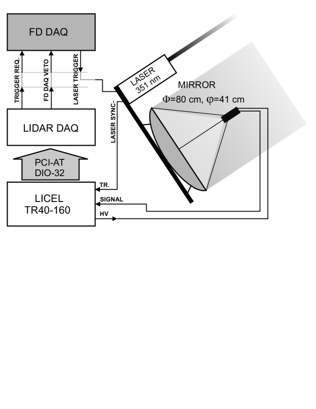
Figure 2: Schematic diagram of the Pierre Auger Observatory lidar system. Each lidar telescope uses a set of three $\varPhi=80\,\mathrm{cm}$ diameter parabolic mirrors with a focal length of $\varphi=41\,\mathrm{cm}$.

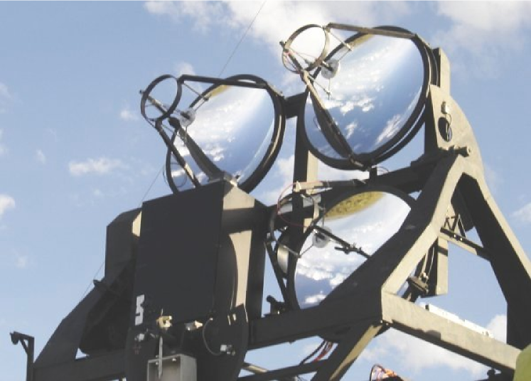
Figure 3: The Los Leones lidar system. Pictured are the 3 mirrors and the box which houses the high frequency laser. The laser shoots from the box in the direction of the field of view of the mirrors.

4 Lidar Hardware and Data Acquisition

As of March 2006, three of the four lidar stations of the Pierre Auger Observatory have been fully operational. The first lidar was installed at the Los Leones site in March 2002 and started data taking soon after, mainly to test the impact on FD operations and define optimal running conditions. The lidar at the Coihueco site began operation in March 2005, and the lidar at the Los Morados site started operation in March 2006. The fourth FD at Loma Amarilla is currently under construction and is expected to be completed by December 2006, with the corresponding lidar station to be operational at the same time. A schematic diagram of a lidar station is shown in Fig. 2. Fig. 3 shows a photograph of the Los Leones lidar setup.

4.1 Mount

Each lidar station has at its core a fully steerable alt-azimuth frame built originally for the EAS-TOP experiment [10]. Two DC servomotors steer the frame axes with a maximum speed of $2^{\circ}/\mathrm{s}$. The absolute pointing direction is known to $0.2^{\circ}$ accuracy.

The frame is mounted on a $20^{\prime}$ shipping container and is protected from the weather by a fully retractable motorized cover during periods when the lidar is not operating. Frame-steering and cover movements are controlled by an MC-204 motion controller from Control Techniques, which allows the system to be operated both locally at the site and remotely via Ethernet.

4.2 Laser

Each mount is equipped with a UV laser source and mirrors for the detection of the backscattered light. The choice of a laser for the lidar system is dictated by the following requirements: the wavelength of the laser has to roughly match the dominant wavelength of air fluorescence photons; the laser power should be low to minimize interference with the FD; and the repetition rate should be high to reduce data collection time. To meet these requirements, the lidars are operated with diode pumped solid state lasers of type DC30-351 manufactured by Photonics Industries. This laser generates the third harmonic of Nd:YLF at 351 nm and is operated at a repetition rate of 333 Hz and a per-pulse energy of roughly $100\,\mathrm{\mu J}$. The laser wavelength of 351 nm is at the center of the nitrogen fluorescence line spectrum, which extends from about 300 nm to 400 nm, with three main spectral lines at 337 nm, 357 nm and 391 nm [11].

4.3 Mirrors

For the collection of the backscattered light, each lidar telescope uses a set of three $\varPhi=80\,\mathrm{cm}$ diameter parabolic mirrors with a focal length of $\varphi=41\,\mathrm{cm}$ (see Fig. 2). The mirrors were produced using BK7 glass coated with aluminum, and the reflective surface is protected with $\mathrm{SiO}_{2}$ coating to ensure the necessary surface rigidness as well as good UV transmittance. The average spot size at the focus is $3\,\mathrm{mm}$ FWHM. Each of the mirrors is mechanically supported by a Kevlar frame which is in turn fixed to the telescope frame using a three point system. This allows fine adjustment of the field of view direction to ensure collinearity of the mirrors and the laser beam.

4.4 Photomultiplier and Digitization

A Hamamatsu R7400U series photomultiplier is used for backscatter light detection. Each mirror has its own photomultiplier, so each lidar telescope comprises three independent mirror/photomultiplier systems. The photomultiplier reaches a gain of $2\times 10^{6}$ at the maximum operation voltage of $1000\,\mathrm{V}$. To facilitate the light collection from the mirror, the whole active $8\,\mathrm{mm}$-diameter photomultiplier window is used.

Background is suppressed by the means of a broadband UG-1 filter with $60\%$ transmittance at $353\,\mathrm{nm}$ and FWHM of $50\,\mathrm{nm}$. The use of far more selective interference filters is unfortunately not possible because the extreme speed $f/0.5$ ($\varphi/\varPhi\simeq 0.5$) of the mirrors leads to a large spread of possible incident angles. As interference filters are very sensitive to the light impact angle, light has to hit the filter almost orthogonally, or else the transmitted wavelength can shift considerably. However, one must bear in mind that the lidar is constructed to operate during FD data taking, which is only possible on moonless nights. A simple absorption filter is therefore sufficient for effective background suppression.

Due to our specific design requirements, a rather long (12 m) signal cable between the photomultipliers and digitizers has to be used. To minimize the signal dispersion as well as RF interference, UVF-303 series military standard cables are used.

The signals are digitized using a Licel TR40-160 three-channel transient recorder. For analog detection the signal is amplified and digitized by a 12 bit 40 MHz A/D converter with 16 k trace length (current mode). At the same time a fast 250 MHz discriminator detects single photon events above a selected threshold voltage (photon counting mode). A combination of current and photon counting measurement is used in the subsequent analysis to increase the dynamic range of the whole system. The Licel recorder is operated using a PC-Linux system through a National Instruments digital input-output card (PCI-DIO-32HS) with the Comedi interface within the ROOT framework.

4.5 Trigger

The lidar is connected to the FD data acquisition (FD DAQ) system by means of three optical fibers. Whenever the lidar system wants to start a measurement, a trigger request is issued to the FD DAQ. In response, a logic pulse of frequency $333\,\mathrm{Hz}$ is generated by the FD GPS clock and transmitted to the laser, which fires a single laser pulse for every trigger. The frequency of $333\,\mathrm{Hz}$ corresponds to the maximum acquisition rate of the digitizer for the given memory depth ($16\,\mathrm{k}$) and sample rate ($40\,\mathrm{MHz}$). The lidar DAQ is triggered by the laser synchronization signal generated at every successful laser shot. Whenever the lidar direction of measurement comes close or into the FD field of view, a veto signal which prevents FD data acquisition can be generated.

The lidar DAQ software is organized in several layers to allow remote or unattended operation as well as integration into the central Auger DAQ system. A run-control program sends the hardware settings and run parameters to the DAQ program through a communication server. The DAQ program controls the Licel and photomultiplier settings (tube gain via high voltage level, photon scaler discriminator level), triggering system, telescope steering and cover operation. Through the DAQ program, the user also controls the shooting directions and the number of laser shots per shooting angle. Current and photon counting traces are summed for 1000 laser shots in the Licel, stored in a ROOT file and sent to the online analysis framework for monitoring.

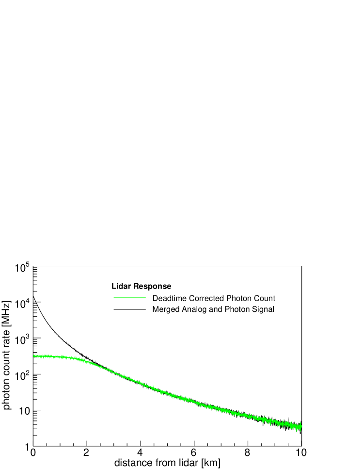
Figure 4: Signals from both current and photon counting mode. The figure shows the backscatter signal up to 10 km distance from the lidar. As long as the photon counting trace is saturated, only the current mode trace is used. When saturation becomes negligible the signal in current mode is fused with the one in photon counting mode.

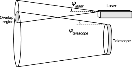
Figure 5: A diagram showing the overlap that occurs in our lidar system, where the laser beam is emitted parallel and outside the field of view of the telescope.

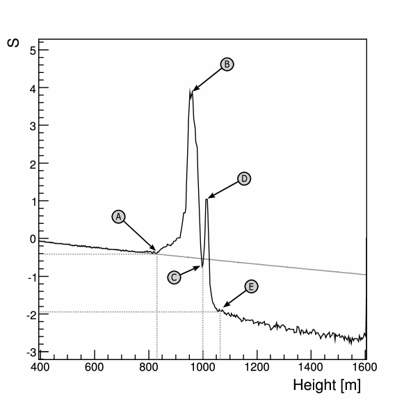
Figure 6: The normalized and range-corrected lidar return $S(h)$. Clouds are seen as strong scattering regions. The first cloud starts at $A$ and shows the maximum peak at $B$. In this example, a second cloud starts at $C$, shows a peak at $D$ and ends at $E$. The grey curve is a simulated lidar response for a purely molecular atmosphere.

4.6 Signal Treatment

As mentioned above, the Licel module records backscattered light measurements in current mode and photon counting mode. Current mode maximizes the near-field spatial resolution, but it is suitable only for the first few kilometers where the signal is sufficiently high. As the signal decreases as the square of the distance, photon counting is required in order to obtain information about the atmosphere at large distances. On the other hand, the photon counting saturates in the near-field due to limitations of the Licel. At distances less than 5 km from the lidar station, the light level causes a rate greater than 10 MHz and the deadtime starts to be an issue ($\geq 5\,\%)$. However, the combination of current and photon counting mode covers the full dynamic range of the return signal from near the detector out to a distance of 25 km. Fig. 4 shows an example for a signal in current and photon counting mode.

In order to combine the current and photon counting signals, the ratio of the two signals is calculated. A range in which this ratio is almost constant is identified, usually when the photon count rate is under 10 MHz, and signals are merged in that region. In the first kilometers this condition is not met due to the fact that the photon counting mode saturates for high photon rates (see Fig. 4). Typically, the optimal merging region is 5-10 km from the detector, where both the current and photon counting signals are valid.

The derived signal can be parameterized by the so-called lidar equation:

$$P(r)=P_{0}\frac{ct_{0}}{2}\beta(r)\frac{A}{r^{2}}e^{-2\tau(r)}=P_{0}\frac{ct_{0}}{2}\beta(r)\frac{A}{r^{2}}e^{-2\int_{0}^{r}\alpha(r^{\prime})dr^{\prime}}\hskip 10.0pt,$$ (3)

where $P(r)$ is the signal received at time $t$ from photons scattered at a distance $r$ from the lidar, $P_{0}$ is the transmitted laser power, $t_{0}$ is the laser pulse duration, $\beta(r)$ is the backscattering coefficient, $\tau(r)$ is the optical depth, $\alpha(r)$ is the extinction coefficient, and $A$ is the effective receiving area of the detector. $A$ is proportional to the overlap of the telescope field of view with the laser beam (shown in Fig. 5). Over the range of distances where the laser beam and mirror viewing field only partially overlap, it is possible to experimentally determine an overlap function from horizontal scans [12]. However, since we restrict our analysis to a range starting at $r_{0}=750$ m, where the overlap is complete, we do not apply an overlap correction.

The far limit $r_{f}$ of our range is defined as the distance at which the signal is negligible as compared to the background, typically 25 km. In the region from $r_{0}$ to $r_{f}$, it is convenient to express the return signal as a function of height $h$ in terms of a range-corrected and normalized auxiliary function, $S(h)$:

$$S(h)=\ln\frac{P(h)h^{2}}{P(h_{n})h_{n}^{2}}=\ln{\frac{\beta(h)}{\beta(h_{n})}}-2\tau(h;h_{n})\sec(\theta)\hskip 10.0pt.$$ (4)

In this equation, $P(h)$ is the signal at height $h$, $\tau(h;h_{n})$ is the optical depth calculated in the range $[h_{n},h]$, and $\theta$ is the lidar inclination angle from the zenith. The normalization height $h_{n}$ is a fixed height to normalize $P$, chosen such that at $h_{n}$, the entire signal is in the field of view of the mirrors.

Clouds are visible as strong localized scattering sources. Fig. 6 shows an example of $S(h)$ in the presence of a cloud layer starting at a height of about 830 m. Also shown is the simulated lidar response for a purely molecular atmosphere. The figure illustrates that it is possible to resolve several layers of clouds. A second cloud layer can be seen at an altitude of about 1000 m. The cloud finding algorithm applied in this analysis is described in detail in Section 6.1.

5 Operation

5.1 Current Status

The lidar stations were designed to be operated remotely from the observatory’s central campus in Malargüe. There, a computer is used to centralize the operation and issue all the startup commands to the three existing lidar stations and also to monitor the quality of the data being collected.

The remote operation of systems with this level of complexity presents a number of challenges. In order to achieve a safe handling of the telescopes, various software routines and hardware devices have been installed to monitor the performance and status of lidar operations. These monitoring subsystems include programs used to collect weather related information (mainly rain and wind speed data). The presence of ambient light and the status of the power supply are monitored as well. In the occurrence of an external event such as rain that could jeopardize the lidar equipment, these subsystems assume control of the station by parking the telescope and closing the cover.

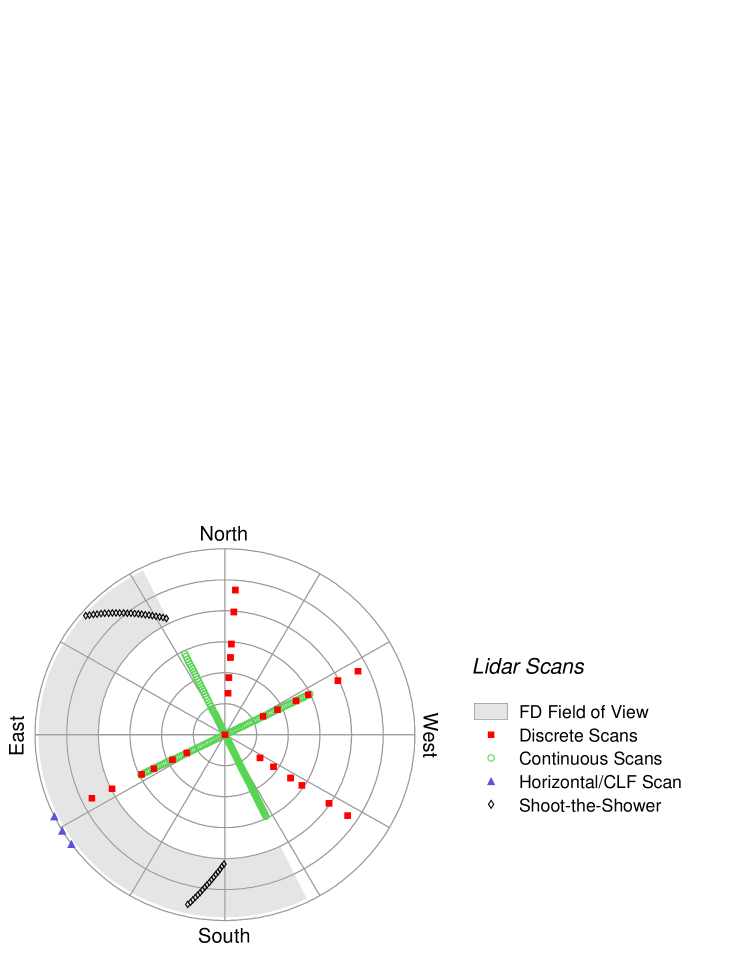
Figure 7: A typical night of lidar shooting activities at Coihueco, shown in an azimuthal equatorial projection of the sky. Depicted are the coordinates for the lidar automatic shooting strategy, which comprises: discrete sweeps for atmospheric parameter estimation; continuous sweeps for cloud detection; horizontal shots toward the Central Laser Facility (CLF) for calibration; and shoot-the-shower scans to probe the tracks of important showers viewed by the fluorescence detector (FD). The Coihueco FD field of view is shown in gray.

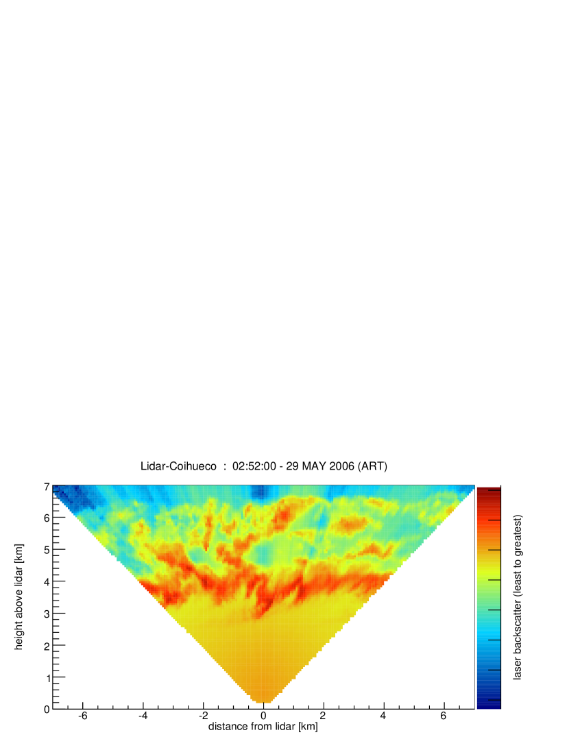
Figure 8: Result of a typical continuous lidar scan. Shown is the intensity of backscattered light as a function of height and horizontal distance to the lidar station at (0,0). A cloud layer around 3.5 km height is clearly visible in this scan.

5.2 Typical Operation

Lidar operation starts at astronomical twilight. After the telescope cover is opened, an initialization procedure is executed to calibrate the incremental encoders used to determine the telescope position.

A webcam located in the interior of the telescope cover is used to confirm visually that these tasks are executed correctly. In this way, before starting a run, the operator has information about the status of the telescope in real time and about the weather conditions at each site through the information being sent to the lidar web site.

Following initialization, the system enters an operational mode called AutoScan. In AutoScan mode, the telescope performs a cycle of steering scripts unless otherwise interrupted until the end of the night. When the laser is fired, the telescope position is determined by the coordinates contained in these scripts. There are four main steering strategies: three making up the AutoScan pattern and a fourth, shoot-the-shower, that periodically interrupts the AutoScan. These strategies are discussed below, and Fig. 7 shows, in an azimuthal equatorial projection of the sky, the firing pattern for a typical night of lidar activities at Coihueco.

• Continuous scans: In this scan, the telescope is moved between two extreme positions with a fixed angular speed while the laser is fired. The telescope sweeps the sky along two orthogonal paths with fixed azimuthal angle, one of which is along the central FD azimuth ($90^{\circ}$). Along both paths, the maximum zenith angle is $45^{\circ}$. The continuous sweeps are constrained to take 10 minutes per path from start to finish. Along each path, the lidar performs on the order of 100 measurements with 1000 shots per measurement. The purpose of these scans is to provide useful data for simple cloud detection techniques (see Section 6.1 for details) and to probe the atmosphere for horizontal homogeneity. An example of the data produced by this kind of scan is shown in Fig. 8.

• Discrete scans: In this scan, the telescope is positioned at a set of particular coordinates to accumulate larger statistics at a few locations. As indicated in Fig. 7, these measurements are performed at 6 discrete zenith angles for 4 different azimuth angles, and directly overhead (zenith angle $0^{\circ}$). To accumulate large statistics, 12 measurements are performed at each location. Each measurement consists of 1000 laser shots run at 333 Hz. The combined duration of the two discrete sweeps is about 30 minutes. The data obtained in this mode are useful to determine the vertical distribution of aerosols in the atmosphere.

• Horizontal and CLF shots: In this mode, the laser fires horizontally in 3 different directions towards the location of the CLF. Three measurements with 1000 shots per measurement are performed. The data collected in this scanning mode are used to detect low-lying aerosols and also to determine the horizontal attenuation between the CLF and the FD telescopes for comparison with measurements made by other atmospheric monitoring systems. The total duration is about 3 minutes.

• Shoot-the-Shower (StS): This rapid response mode is used to measure the atmospheric attenuation in the line of sight between the FD telescopes and a detected cosmic ray shower. This scanning mode suspends any of the previously mentioned sweeps. It will be described in further detail in section 5.2.

A complete scanning cycle, excluding StS, takes about 60 minutes to complete. All scans are therefore performed on an hourly basis. The maximum length of a lidar running night depends on the length of astronomical twilight and varies over the course of the year from less than five hours during the summer to almost fourteen hours during the winter.

As shown in Fig. 7, some shooting positions are very close to or inside the field of view of the FD telescopes. In order to prevent the detection of a large number of spurious FD events generated by the lidar shooting activity, buffer zones have been delimited around the FD fields of view. Every time the laser is fired inside this buffer zone, the FD DAQ is inhibited in order to avoid any interference. This is accomplished by sending a veto signal from the lidar to the FD when the laser is ready to fire. The total FD deadtime introduced by all lidar operations is less than $2\,\%$.

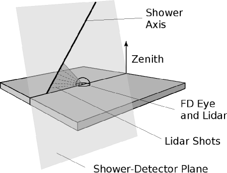
Figure 9: The geometry of shoot-the-shower (StS). The lidar station at a fluorescence detector site initiates shots in the shower-detector plane within the zenith field of view of the FDs (approximately $\it 0^{\circ}$ to $\it 30^{\circ}$ in elevation). Up to 60 pointing directions, with 1000 laser shots per pointing, are allowed per StS.

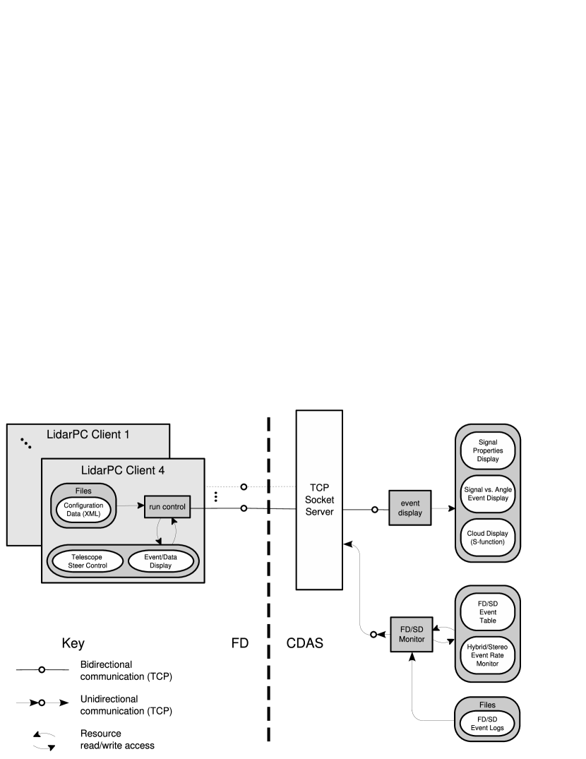
Figure 10: Communication between the Pierre Auger Observatory central data acquisition system (CDAS) and the independent lidar stations running in each FD subnetwork. A data monitoring client in CDAS checks for hybrid and stereo events; via TCP, it sends StS requests to the LidarPCs, where the lidar run control program executes shoot-the-shower.

5.3 Shoot-the-Shower

A primary design requirement of the lidar system is that it probe the atmosphere along the tracks of cosmic rays observed by the FDs. This function, called shoot-the-shower (StS), exists to recognize unusual and highly localized atmospheric conditions in the vicinity of individual air showers of high interest. Conditions that can affect FD observations at different times of the year include the presence of low and fast clouds, and low-level aerosols due to fog, dust, or land fires.

The basic operation of StS is depicted in Fig. 9. The axis of a cosmic ray air shower, when projected onto the field of view of an observing air fluorescence detector, defines a plane called the shower-detector plane, or SDP. When a lidar station shoots the shower, it performs a series of laser shots within this plane, determining the atmospheric transmission between the shower segment and the FD. For a given shower, up to 60 pointing directions with 1000 laser shots per pointing are allowed, all within the FD field of view.

To operate effectively, the lidar must shoot showers of importance with a minimum of delay after each shower occurs and with minimum disruption to the normal operation of the FD. The showers of primary interest for StS are hybrid events involving the FDs and the SD, since these set the energy scale of the observatory. FD stereo events, which are of high energy and typically at large distances from the FDs, are also good StS candidates.

Physics events are made available to the lidar by picking off the SD and FD data stream sent continuously to the observatory’s central data acquisition system (CDAS), located on the central campus. A program running in CDAS monitors incoming data, checks for hybrid and stereo events, and calculates StS trajectories. StS requests are sent to the lidar station data acquisition and control PCs (LidarPCs), which initiate the laser shots.

Communication between the lidar stations and CDAS, shown schematically in Fig. 10, occurs over the network links between the central campus and the four FD subnetworks. Each LidarPC listens on an open TCP port for StS requests from the FD/SD monitor running in CDAS. As the lidar shoots, it returns basic diagnostic information, such as shooting directions and PMT signal peaks, back to CDAS for display. A TCP socket server operating in CDAS manages the bidirectional flow of data packets between the central campus and the lidar stations.

Lidars receiving StS requests from CDAS automatically stop the default shooting operation (AutoScan), move to the FD field of view, initiate the StS, and then resume the AutoScan when StS is complete. If the lidar receives an StS request while shooting another shower, the request is pushed into a queue for later processing.

To minimize the FD dead-time introduced by StS, the lidar software cuts on the number of SD tanks participating in the event, which is a rough measure of the primary cosmic ray energy. This cut reduces the number of requests to several per FD site per night. A further reduction in the rate is achieved by rejecting events caused by known artificial light sources in the detector, such as other lidar stations and the CLF. In addition, the intensity of the high-repetition laser means that the lidar must carefully avoid incidents of cross fire into other unvetoed FDs during StS. Therefore, angular windows in azimuth and in zenith are defined around each FD; the lidar is forbidden from entering these windows during StS.

The operation of StS in the field of view of the photomultiplier cameras raises the issue of possible long term effects on the phototubes themselves. Although FD data acquisition is inhibited during StS, the photomultipliers continue to operate at high voltage during their exposure to powerful nearby laser shots. However, since the shooting rate is one to two shots per FD per night, the effect of the StS is not significant in comparison to other strong and persistent light sources. These sources include the typical night sky background with its large number of bright stars, and heavy lightning activity during the summer months. In addition, a comparison of tube noise directly before and after StS events shows no significant effect of the shooting activity on the tube noise.

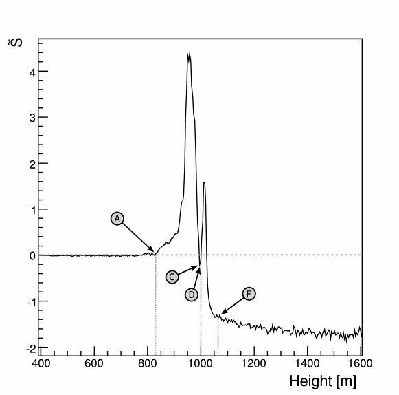
Figure 11: The normalized and range-corrected lidar return $S(h)$ after subtraction of a simulated return that assumes a purely molecular atmosphere.

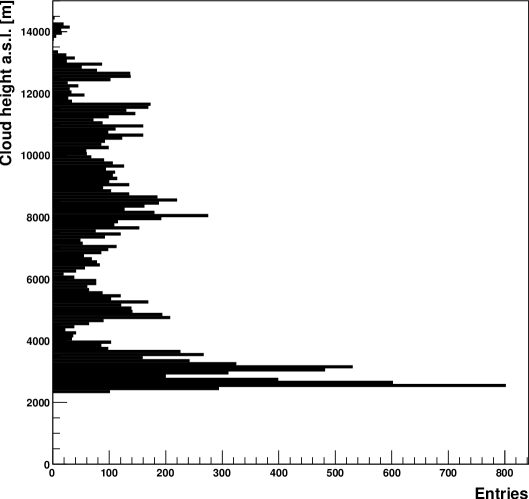
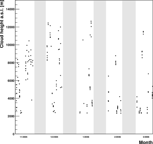
Figure 12: Distribution of the height above sea level (a.s.l.) of the lowest cloud layer (upper plot), and height of the lowest cloud layer as a function of time (lower plot) for data taken between 24 October 2005 and 7 March 2006 with the Coihueco lidar. The grey areas in the lower plot indicate the periods when the moon is too bright for FD data taking. The plots have 1 entry for each hour when a cloud was detected.

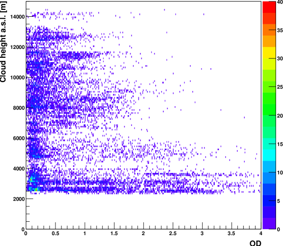
Figure 13: Height above sea level (a.s.l.) of the lowest cloud layer versus vertical aerorosal optical depth inside the lowest cloud layer observed by the Coihueco lidar between 24 October 2005 and 7 March 2006.

6 Analysis

In standard operation mode, the two goals of the lidar system are (1) to provide hourly measurements of vertical aerosol optical depth and backscatter coefficient as a function of height at each FD site, and (2) to provide hourly information on cloud coverage, cloud height, and the optical depth of cloud layers. The analysis of lidar scans to extract the vertical aerosol optical depth is discussed in detail in [8]. Here, we will describe the analysis of cloud coverage and optical depths of cloud layers. These measurements are particularly important for the accurate estimation of the FD detection aperture. While they do not affect the SD aperture, clouds within the fields of view of the FDs distort the light profile of showers and can compromise the energy calibration.

6.1 Cloud Detection

As described in Section 4.6, clouds are detected as strong localized scattering sources, and the timing of the backscattered light gives the distance from the cloud to the lidar. The return signal is expressed in terms of the $S$ function (Eq. 4).

To automatically detect clouds, it is useful to calculate a new function $\tilde{S}(h)$ by subtracting the $S$ function for a simulated purely molecular atmosphere from the measured $S$ function:

$$\tilde{S}(h) = S-S_{mol}$$ (5)

$$= S-\ln{\left[\frac{\beta_{mol}(h)}{\beta_{mol}(h_{n})}\right]}+2\tau_{mol}(h;h_{n})\sec(\theta)$$

$$= \ln{\left[\frac{\beta(h)}{\beta(h_{n})}\frac{\beta_{mol}(h_{n})}{\beta_{mol}(h)}\right]}-2\tau_{aer}(h;h_{n})\sec(\theta)\hskip 10.0pt,$$

where $h_{n}$ is the normalization height (as in Eq. 4), $\beta(h)$ is the backscattering coefficient, $\tau(h;h_{n})$ is the optical depth calculated in the range $[h_{n},h]$, and $\theta$ is the lidar inclination angle from the zenith.

The properties of the molecular atmosphere at the Pierre Auger Observatory site are very well-known thanks to an extensive balloon-launching program which has produced a detailed database including temperature, pressure, and density profiles over the site [13]. Data from these balloon flights, typically performed every 5 days, are used to create monthly models of the molecular atmosphere at the Malargüe site. In the lidar analysis we use these monthly models for the calculation of $\tilde{S}(h)$. By using the monthly models, seasonal variations in the molecular atmosphere are accounted for, but day-to-day variations, which can be substantial [14], are not. These short term variations do not affect the cloud finding algorithm, and their effect on the calculation of the optical depth of the cloud layer is negligible. As shown in Fig. 11, $\tilde{S}(h)$ is approximately constant before the cloud, and has a non-zero slope inside the cloud. We apply a second-derivative method [15] to identify cloud candidates and obtain the cloud thickness.

In cases where several cloud layers are present, the influence of partial overlaps between cloud layers causes an inaccurate estimation of the optical depth of the first cloud. For this reason, very near clouds separated by less than 10 m are treated as a single cloud layer, and the optical depth is calculated only for the combination of the layers.

In order to reduce the possibility of a spurious cloud detection, we take advantage of the fact that each lidar has three individual mirrors and photomultipliers, so the same signal is detected independently several times. To discriminate against noise, we require a cloud to be detected in multiple mirrors. Signals from different mirrors of the same lidar are therefore compared before a cloud is stored and a cloud detection is reported.

6.2 Optical Depth of the Cloud Layer

The application of the cloud detection algorithm to lidar scans can provide a variety of useful data. Collecting all the scans during an hour, the lowest layer of clouds is identified and the proportional sky coverage is calculated. Fig. 12 shows the distribution of the height of the lowest detected cloud layer (upper plot) and the height of the lowest layer as a function of time (lower plot) for data taken between 24 October 2005 and 7 March 2006 with the Coihueco lidar. Typical cloud layers can be identified, in particular a recurrent cloud layer between 2000 m and 3000 m above sea level.

Once the lowest clouds have been identified, their effect on the light propagation is estimated. The turbidity of a layer of thickness $H$ can be described by a transmission factor

$$T(H)=e^{-\tau(H;0)}\hskip 10.0pt,$$ (6)

where $\tau(H;0)$ is the total optical depth.

Consider, for instance, a cloud at a height $h_{A}$ that ends at a height $h_{F}$. From a lidar scan, the auxiliary function $S(h)$, given by Eq. 4, is obtained, and $\tilde{S}(h)$ is calculated by using Eq. 5. The difference between the values assumed by $\tilde{S}(h)$ in $h_{A}$ and $h_{F}$ is:

$$\Delta\tilde{S}(h_{F};h_{A})=\ln{\left[\frac{\beta(h_{F})}{\beta_{mol}(h_{F})}\frac{\beta_{mol}(h_{A})}{\beta(h_{A})}\right]}-2\tau_{aer}(h_{F};h_{A})\sec{\theta}\hskip 10.0pt,$$ (7)

where $\tau_{aer}(h_{F};h_{A})$ is due to scattering and absorption of the light by the cloud.

At heights greater than 2 km above ground level a quasi-molecular atmosphere can be assumed in the proximity of clouds. Therefore, $\beta\simeq\beta_{mol}$ at $h_{A}$ and $h_{F}$, and Eq. 7 becomes:

$$\Delta\tilde{S}(h_{F};h_{A})\simeq-2\tau_{aer}(h_{F};h_{A})\sec{\theta}\hskip 10.0pt.$$ (8)

In this way, the cloud optical depth can be estimated directly from the signal:

$$\tau_{aer}(h_{F};h_{A})\simeq-\frac{1}{2}\Delta\tilde{S}(h_{F};h_{A})\cos(\theta).$$ (9)

Using this information, the mean optical depth inside the lowest cloud layer is calculated for every hour of FD data taking. As an example of the capability of the lidar system to detect and characterize clouds, Fig. 13 shows the height of the lowest cloud layer versus the optical depth inside the lowest cloud layer observed with the Coihueco lidar between 24 October 2005 and 7 March 2006. The plot indicates that low altitude clouds tend to cover a wider range of optical depths than clouds at higher altitude.

The atmospheric monitoring facilities of the Pierre Auger Observatory also include customized infrared cloud cameras at each FD site [1]. These cameras scan the entire sky every 15 minutes. The pictures are processed and used to fill a database with information on the cloud coverage. To first order, the images from the cloud camera provide a crude cross-check of the efficiency of the lidar cloud finding algorithm. In practice, the two cloud analyses are complementary, with the lidar providing the height and optical properties of cloud layers and the cloud cameras providing a complete two-dimensional image of the cloud coverage.

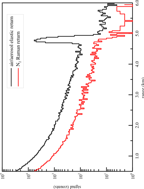
Figure 14: Comparison of the lidar returns in the elastic and nitrogen channels. A cloud layer at about 4.8 km height appears as an attenuation in the nitrogen channel, but as an increase in the signal in the elastic channel due to the enhanced backscattering.

7 Inelastic Raman Lidar

7.1 Principle of Operation

In addition to operating the elastic backscatter lidars, the Pierre Auger collaboration is currently also evaluating the usefulness of a Raman lidar operated in conjunction with the elastic lidar at Los Leones.

The Raman technique is based on inelastic Raman scattering, a secondary component of molecular scattering in the atmosphere. The inelastic component is suppressed compared to elastic Rayleigh scattering since the Raman scattering cross section is about three orders of magnitude smaller than the corresponding Rayleigh cross section. In Raman scattering, the scattered photon suffers a frequency shift that is characteristic of the stationary energy states of the irradiated molecule. With Raman spectroscopy, it is therefore possible to identify and quantify traces of molecules in a gas mixture.

Raman lidars operate on the same principle as elastic lidars, except that Raman lidars feature a spectrometer-type receiver to discriminate the lidar returns according to wavelength. Our receiver has 3 channels to detect the light intensity at various wavelengths. One channel collects the elastic lidar return, while the others correspond to the atmospheric oxygen and nitrogen Raman lidar backscatter, at about 375 nm and 387 nm, respectively.

The Raman lidar technique overcomes a major weakness of the elastic lidar measurements, in which the aerosol scattering contribution is present both in the transmission and backscattering components. Extracting the aerosol attenuation from elastic lidar data therefore requires some assumptions regarding aerosol optical properties, mainly the relationship between aerosol backscatter and extinction. For the Raman lidar, the aerosol scattering contribution is only present in the transmission, so the only assumption to be made is the wavelength dependence of the aerosol transmission coefficient. If the Raman lidar returns are measured for several wavelengths simultaneously, for example for molecular nitrogen and oxygen, even the wavelength dependence can in principle be retrieved without any assumptions. In addition, if the elastic signal at the laser wavelength is measured simultaneously, a comparison between the elastic Rayleigh and inelastic Raman return can be used to give an independent estimate of the aerosol content as a function of height.

A practical disadvantage of the Raman lidar technique is the small Raman molecular cross section. As a consequence, the laser source has to be operated at high power and care has to be taken not to disturb the FD operation. Currently, Raman lidar runs at the Pierre Auger Observatory are only performed right before and after the regular FD operation.

7.2 Raman Lidar Hardware and Data Acquisition

The Raman lidar system consists of a Nd:YAG laser (ULTRA CFR) manufactured by Big Sky Laser Technologies, Inc. The emitted pulses at 355 nm have a line width of $<3\,\mathrm{cm}^{-1}$, a pulse energy of about 10 mJ at a repetition rate of 20 Hz, and a pulse duration of about 6 ns. The full angle divergence is less than 1 mrad. The emitted laser pulses are directed in the atmosphere (zenith direction) with a $2^{\prime\prime}$ steering mirror, which has a pointing sensitivity of about 0.1 mrad.

The Raman lidar has to meet a few general requirements. It must be capable of sampling a range of altitudes from the ground to 7000 m, be optimized to detect weak Raman backscattering from atmospheric nitrogen and oxygen, and efficiently suppress background light and cross-talk between the different channels.

These conditions impose restrictions on the choice of the receiving optics, and on the design of the dichroic beam splitters and interference filters to be used in the wavelength discriminating detectors. They also impose the use of notch filters providing an additional suppression of the strong elastically backscattered light in the Raman channels.

In the setup of the Raman lidar system, the backscattered light is collected by a zenith pointing telescope (50 cm diameter parabolic mirror, focal length 150 cm) through a 10 m long multi mode optical fiber coupled to the telescope with an aspherical lens. The fiber transports the return light to the 3-channels beam separator: a combination of beam splitters, interference filters, notch filters, and neutral density filters.

After passing the final stage of the beam separator unit, the light is collected by Hamamatsu R1332 photomultipliers. The voltage pulses at the output of the photomultipliers are amplified by a fast pre-amplifier (EG&G Ortec, model 535). A discriminator (CAEN N224) reduces the dark counts and forms 30 ns wide NIM pulses. These pulses are detected by a PXI-5620 digitizer (National Instruments, maximum sampling rate 64 Msample/s) usually in a 0.200 ms time window (30 km range). The number of pulses in each of 1000 time windows (200 ns wide, corresponding to a distance resolution of 30 m) are counted, stored and displayed in a personal computer, after summing over a number of laser shots. The maximum counting rate is kept below 10 MHz so that pulse pile-up effects are negligible. The data production is presently quite small: 576 kByte for 40 minutes of data taking.

Fig. 14 shows the typical returns in the elastic and nitrogen/Raman channels. Note that the presence of a cloud layer at about 4.8 km height appears as an attenuation in the Raman lidar return, since, as described above, the aerosol scattering is only present in the transmission. In the elastic lidar signal, on the other hand, the cloud appears as an increase in the signal due to the enhanced backscattering.

The Raman lidar is remotely operated, sharing some services with the elastic lidar already operating at Los Leones. Currently, the main goal of the Raman lidar is to measure the vertical aerosol optical depth. Since the Raman measurements have to be taken outside FD operations, the measurement obtained with this technique is not directly usable for the analysis of FD data. However, it can be used to cross-check and validate the estimates of the aerosol content made by the subsequent elastic lidar operation.

8 Conclusions and Outlook

Since March 2006, three of the four lidar stations are routinely operated each night of FD data taking by a designated lidar shift taker at the central campus. The fourth site is currently under construction and will start data taking in 2007. The three operating lidars perform continuous and discrete scans of the local atmosphere, and the data are analyzed for cloud coverage, cloud height, and the optical depth of cloud layers. An analysis of the aerosol scattering and absorption parameters will be added in the near future.

As the part of the lidar program that has the largest potential to interfere with the FD operation, the shoot-the-shower program is still in a testing phase. Algorithms to maximize the efficiency of StS are currently under development. This includes the implementation of software to filter background events that can erroneously trigger the StS, such as lightning.

As a possible future extension of the elastic backscatter lidar program, an inelastic Raman lidar is operated at the beginning of each data taking night.

Another future upgrade currently under consideration is the installation of new mirrors with a larger focal length to reduce the speed of the lidar optics. The large field of view of the current system implies that the background rate is high and the laser beam enters the field of view of the mirrors very early. To lower the amount of background light and overcome saturation at short range, a segmented mirror with a 1 m diameter and 1.1 m focal length is currently under development.

References

- [1] R. Cester (for the Pierre Auger Collaboration), Atmospheric Monitoring at the Pierre Auger Observatory, in Proc. Int. Cosmic Ray Conference, Pune, India (2005).
- [2] P. Mantsch (for the Pierre Auger Collaboration), The Pierre Auger Observatory Status and Progress, in Proc. Int. Cosmic Ray Conference, Pune, India (2005) (astro-ph/0604114).
- [3] M.D. Roberts, J. Phys. G: Nucl. Part. Phys 31 (2005) 1291.
- [4] A. Bucholtz, Appl. Opt. 34 (1995) 2765.
- [5] G. Mie, Ann. Phys. 25 (1908) 377.
- [6] H.C. van de Hulst, “Light Scattering by Small Particles,” Wiley, New York (1957).
- [7] E.J. McCartney, “Optics of the Atmosphere: Scattering by Molecules and Particles,” Wiley, New York (1976).
- [8] A. Filipčič, M. Horvat, D. Veberič, D. Zavrtanik, and M. Zavrtanik, Astropart. Phys. 18 (2003) 501.
- [9] B. Fick et al., Journal of Instrumentation 1 (2006) P11003.
- [10] M. Aglietta et al., Nuovo Cimento 16 (1993) 813.
- [11] F. Kakimoto et al., Nucl. Instr. Meth. A 372 (1996) 527.
- [12] Y. Sasano, H. Shimizu, N. Takeuchi, and M. Okuda, Appl. Opt. 18 (1979) 3908.
- [13] J. Blümer et al. (for the Pierre Auger Collaboration), Atmospheric Profiles at the Southern Pierre Auger Observatory and their Relevance to Air Shower Measurement, in Proc. Int. Cosmic Ray Conference, Pune, India (2005).
- [14] B. Wilczyńska et al., Variability of Atmospheric Depth Profiles, in Proc. Int. Cosmic Ray Conference, Pune, India (2005).
- [15] A. Tonachini, PhD thesis, University of Torino, in preparation.