Unstable modes of non-axisymmetric gaseous discs

Abstract

We present a perturbation theory for studying the instabilities of non-axisymmetric gaseous discs. We perturb the dynamical equations of self-gravitating fluids in the vicinity of a non-axisymmetric equilibrium, and expand the perturbed physical quantities in terms of a complete basis set and a small non-axisymmetry parameter $\epsilon$. We then derive a linear eigenvalue problem in matrix form, and determine the pattern speed, growth rate and mode shapes of the first three unstable modes. In non-axisymmetric discs the amplitude and phase angle of travelling waves are functions of both the radius $R$ and the azimuthal angle $\phi$. This is due to the interaction of different wave components in the response spectrum. We demonstrate that wave interaction in unstable discs with small initial asymmetries, can develop dense clumps during the phase of exponential growth. Local clumps, which occur on the major spiral arms, can constitute seeds of gas giant planets in accretion discs.

1 Introduction

Unstable density waves inside self-gravitating gaseous media play an important role in structuring of spiral galaxies and accretion discs. Prior works in the literature deal with the instability of differentially rotating discs, which are initially circular. Aoki et al. (1979) carried out a global analysis of spiral modes in the soft-centred, gaseous Kuzmin (1956) disc using Hunter’s (1963) device. Lemos et al. (1991) studied the unstable axisymmetric modes of the more puzzling scale-free discs and solved the dispersion relation to determine the sufficient conditions for ring formation and for the existence of breathing modes. Recently Goodman & Evans (1999, hereafter GE) constructed the normal modes of the scale-free Mestel (1963) disc in the Cowling approximation. For self-gravitating modes they computed the ratio of growth rate to pattern speed by solving a recurrence relation in the Mellin-transform space. Density waves in the presence of an external potential field, like that of a massive central object, have also been extensively studied using semi-analytical and finite difference techniques (e.g., Papaloizou & Lin 1989; Savonije & Heemskerk 1990; Papaloizou & Savonije 1991).

The assumption of axisymmetry of the equilibrium (or initial) state, however, imposes significant simplifications on the solution of dynamical equations. In fact, unstable modes of circular discs are decoupled because the only $\phi$-dependent term, $\exp({\rm i}m\phi)$ (${\rm i}=\sqrt{-1}$), is factored out of the linearized Poisson and hydrodynamic equations. Here $\phi$ is the azimuthal angle and $m$ is the wave number. Such a factorization is impossible if the unperturbed state is non-axisymmetric. Azimuthal modes of perturbed non-axisymmetric discs can interact with the Fourier components of the equilibrium state and result in more complex patterns.

In this paper we attempt to formulate the instability problem of non-axisymmetric discs based on a perturbation theory, and present a mechanism for the generation of dense clumps through wave interaction in linear regime. That occurs when a non-axisymmetric disc is destabilized. We apply our formulation to the simple discs of Jalali & Abolghasemi (2002, hereafter JA), which reduce to Mestel’s disc in axisymmetric limit. We have chosen JA models as our unperturbed state because of two reasons. Firstly, closed form (exact) expressions are available for physical quantities like the potential–density pair, pressure, sound speed and velocity components. Secondly, both the potential and the surface density have a single Fourier component. This minimizes the number of interacting terms in our subsequent analysis.

We review steady-state, non-axisymmetric, scale-free discs of JA in section 2 and introduce a cutout function that helps us handle the singularity at the centre. We present a first-order perturbation theory for non-axisymmetric gaseous discs in section 3, where we also introduce a basis set by which we expand the perturbed physical quantities. We then derive an eigenvalue problem for determining the normal modes of non-axisymmetric discs and discuss on the algorithms used for solving the resulting eigensystem. In sections 4 and 5, we study the unstable modes of circular and non-axisymmetric discs for the fundamental wave numbers $m=0$, 1 and 2, and discuss on the results and their physical implications in section 6.

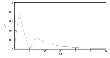
Figure 1: The region under the solid line is the allowable zone in the parameter space of a bisymmetric disc with $n=2$.

2 Non-axisymmetric gaseous discs in equilibrium

There are few papers in the literature that address non-axisymmetric equilibria of gaseous discs (Syer & Tremaine 1996; Galli et al. 2001; JA). In this section we briefly review one of exact non-axisymmetric models of JA whose surface density consists of a simple harmonic function of the azimuthal angle.

2.1 Basic derivations

We define $(R,\phi)$ as the usual polar coordinates and assume a self-gravitating, inviscid, compressible fluid in a steady two dimensional state so that the surface density distribution and its self-consistent potential are scale-free as

$$\Sigma\left(R,\phi\right) = \Sigma_{s}\frac{R_{0}}{R}f(\phi),$$ (1)

$$\Phi\left(R,\phi\right) = v_{0}^{2}\left[\ln\frac{R}{R_{0}}+\frac{1}{2}g\left(\phi\right)\right],~{}~{}v_{0}^{2}=2\pi G\Sigma_{s}R_{0}.$$ (2)

Here $G$ is the constant of gravitation, and $R_{0}$ and $\Sigma_{s}$ are the normalizing constants of the length and surface density, respectively. Our discs are non-axisymmetric because $\Sigma$ and $\Phi$ depend on the azimuthal angle $\phi$. Due to the continuity of physical quantities in the azimuthal direction, the functions $f(\phi)$ and $g(\phi)$ are $2\pi$-periodic in $\phi$. For the sake of simplicity, we work with non-axisymmetric discs of the form

$$f\left(\phi\right)=1+\epsilon\cos n\phi,$$ (3)

where $0\leq\epsilon<1$. The $\phi$-dependent part of the potential reads

$$g\left(\phi\right)=-\frac{2}{n}\epsilon\cos n\phi.$$ (4)

For $\epsilon=0$, our discs reduce to the isothermal, gaseous Mestel disc. Let us respectively define $c_{0}$, $V_{c}$ and $M$=$V_{c}/c_{0}$ as the sound speed, velocity of circular orbits and Mach number in Mestel’s disc. The components of the velocity field associated with (1) and (2) are obtained after solving the hydrodynamic equations as (JA)

$$v_{\phi}(\phi)\!\!\! = \!\!\!\frac{V_{c}}{1+\epsilon\cos n\phi},$$ (5)

$$v_{R}(\phi)\!\!\! = \!\!\!-\epsilon\frac{1+M^{2}}{2M^{2}}V_{c}\left(\frac{2\sin n\phi}{1+n}-\frac{\epsilon\sin 2n\phi}{4n^{2}-1}\right).$$ (6)

The sound speed $c(\phi)$ and the pressure distribution $P(\phi)$ are then given by

$$c(\phi)\!\!\!\! = \!\!\!\!c_{0}\sqrt{{(1+M^{2})A(\phi)-2M^{2}\over 2\left(1+\epsilon\cos n\phi\right)^{2}}},$$ (7)

$$P(\phi)\!\!\!\! = \!\!\!\!c^{2}\Sigma,$$ (8)

$$A(\phi)\!\!\!\! = \!\!\!\!2\left(1+\epsilon\cos n\phi\right)\left(1+\frac{\epsilon\cos n\phi}{1+n}+\frac{n\epsilon^{2}\cos 2n\phi}{4n^{2}-1}\right).$$ (9)

$c$ reduces to $c_{0}$ in the limit of $\epsilon=0$. From (2) and (8), and equation (2) in JA, one can verify that $v_{0}^{2}$=$V_{c}^{2}+c_{0}^{2}$. Sound waves are determinate if the pressure is positive, i.e., $c^{2}>0$. A necessary and sufficient condition for the positiveness of $P$ is

$$0<\frac{2M^{2}}{1+M^{2}}<A_{\rm min}.$$ (10)

Here $A_{\rm min}$ is the minimum of $A(\phi)$ over the interval $0\leq\phi\leq 2\pi$. Inequality (10) restricts model parameters. JA models allow for transonic flows because the sound speed depends on $\phi$ and it varies along a given streamline. In principle, transition from subsonic to supersonic speeds can take place smoothly but the reverse phenomenon is impossible without a shock wave. To avoid shock waves, we follow JA and exclude transonic flows from our calculations and investigate supersonic and subsonic discs.

In this paper we choose a bisymmetric equilibrium with $n=2$. The allowable region of the parameter space $(M,\epsilon)$ is determined based on two requirements. Firstly the square of the sound speed must be positive. Secondly, transonic flows are excluded. Fig. 1 shows the admissible zone of the parameter space. Note that for $\epsilon>0$ the Mach number is a function of the azimuthal angle:

$$\textbf{M}(M,\epsilon,\phi)={\sqrt{v_{R}^{2}+v_{\phi}^{2}}\over c(\phi)}.$$ (11)

In the limit of circular discs ($\epsilon=0$) we obtain $\textbf{M}=M$ as expected.

2.2 Active surface density

We are studying scale-free gaseous discs whose surface density and potential diverge near the center according to (1) and (2). The linear stability problem of scale-free discs is ill-posed unless one decides on the way that inward traveling waves are reflected off the cusp. Several methods have been devised to tackle this problem. For scale-free stellar discs Zang (1976) (see also Evans & Read 1998a,b) used an inner cutout, which carves out the density function and deactivates the central region of the stellar system. In this way, stars with high orbital frequencies do not participate in perturbations. For the gaseous Mestel disc GE used a hard internal boundary that fixes the phase with which waves are reflected from the centre. In this paper we apply Evans & Read’s (1998a) method to our cuspy gaseous discs of §2.1 and deactivate some parts of the disc mass by the cutout function

$$H(R)={R^{N_{\rm in}}\over\left[R^{N_{\rm in}}+(\alpha R_{0})^{N_{\rm in}}\right]}{R_{0}^{N_{\rm out}}\over\left[(\gamma R)^{N_{\rm out}}+R_{0}^{N_{\rm out}}\right]}.$$ (12)

We then analyze the perturbations of the active density

$$\Sigma_{\rm act}(R)=\Sigma(R)H(R).$$ (13)

Here $R_{\rm in}=\alpha R_{0}$ and $R_{\rm out}=R_{0}/\gamma$ are the inner and outer cutout radii, respectively. Since the cutout is not applied to the potential, the immobile mass will resemble a rigid bulge/halo component that does not participate in the disc dynamics, but it contributes to the force field. Instability properties are not sensitive to the choice of $R_{\rm out}$. We apply the outer cutout for computational convenience and use a large $R_{\rm out}$ far beyond the region that instabilities occur. The nature of functions by which we will expand perturbed fields, constrains the feasible values of $N_{\rm in}$ and $N_{\rm out}$. We have used $N_{\rm in}$= $N_{\rm out}=2$ throughout this paper.

3 Perturbation theory of non-axisymmetric discs

We define $\textbf{u}=\left(u_{1},u_{2},u_{3}\right)^{T}\equiv(\Sigma,v_{R},v_{\phi})^{T}$ and consider the first order Eulerian perturbations of physical quantities as

u $$\rightarrow \textbf{u}_{0}(R,\phi)+\textbf{u}_{1}(R,\phi,t),$$

$$\Phi \rightarrow \Phi_{0}(R,\phi)+\Phi_{1}(R,\phi,t),$$ (14)

$$P \rightarrow c^{2}(\phi)\Sigma_{0}(R,\phi)+c^{2}(\phi)\Sigma_{1}(R,\phi,t).$$

The superscript $T$ denotes transpose and the subscripts 0 and 1 refer to the equilibrium and perturbed states, respectively. We assume that the perturbed quantities, $\delta_{1}$$\equiv$$\left(\Phi_{1},\Sigma_{1},v_{R1},v_{\phi 1}\right)^{T}$, are composed of a discrete set of normal modes, each of the form

$$\delta_{1,m}(R,\phi,t,\epsilon)\!\! = \!\!e^{-{\rm i}\omega_{m}t}\delta^{(m)}_{1}(R,\phi,\epsilon),$$ (15)

$$\omega_{m}\!\! = \!\!\Omega_{m}+{\rm i}s_{m},~{}~{}{\rm i}=\sqrt{-1},$$ (16)

where $\omega_{m}$, $\Omega_{m}$ and $s_{m}$ are respectively the eigenfrequency, pattern speed and growth rate of the $m$th mode. It is remarked that the real part of $\delta_{1,m}$ gives the physical solution.

We use the equilibrium fields of §2 and substitute from (14) into the continuity and momentum equations of self-gravitating fluids [equations (1E-3) and (6-20) in Binney & Tremaine 1987]. After collecting the first-order terms in perturbed variables, we obtain

$${\bf L}\cdot\textbf{u}_{1}=-\left(0,\partial_{R}\Phi_{1},R^{-1}\partial_{\phi}\Phi_{1}\right)^{T},$$ (17)

with $\partial_{\mu}=\partial/\partial\mu$. The elements of the linear operator ${\bf L}=[L_{ij}]$, ($i,j=1,2,3$), have been given in Appendix A. $\Phi_{1}$ and $\Sigma_{1}$ should also satisfy Poisson’s integral

$$\Phi_{1}=-G\int\int{\Sigma_{1}R^{\prime}{\rm d}R^{\prime}{\rm d}\phi^{\prime}\over\sqrt{R^{2}+R^{\prime 2}-2RR^{\prime}\cos(\phi-\phi^{\prime})}}.$$ (18)

Modes of non-axisymmetric discs bifurcate from those of circular discs once we let $\epsilon$ grow from zero. Therefore, we seek for a perturbation solution for $\delta_{1,m}$ in terms of the non-axisymmetry parameter $\epsilon$. Moreover, continuity of physical quantities in the azimuthal direction implies the periodicity conditions

$$\textbf{u}_{0}(R,\phi+2\pi)\!\!\! = \!\!\!\textbf{u}_{0}(R,\phi),$$ (19)

$$\delta^{(m)}_{1}(R,\phi+2\pi,\epsilon)\!\!\! = \!\!\!\delta^{(m)}_{1}(R,\phi,\epsilon).$$ (20)

These requirements suggest to represent $\textbf{u}_{0}$ by the Fourier series

$$\textbf{u}_{0}(R,\phi)=\sum_{p=-\infty}^{+\infty}\epsilon^{|p|}e^{{\rm i}np\phi}\textbf{u}_{0,p}(R),$$ (21)

and propose the Ansatz

$$\delta^{(m)}_{1}(R,\phi,\epsilon)=\sum_{l=-\infty}^{+\infty}\epsilon^{|l|}e^{{\rm i}(m+nl)\phi}\hat{\delta}^{(m+nl)}_{1}(R).$$ (22)

Using equations (21) and (22) and substituting from (15) in (17), we obtain the determining equation of the $m$th mode as

$$- \!\!\!\!\!\left({{\rm i}\omega_{m}R_{0}\over c_{0}}\right)\hat{\textbf{u}}^{(m+nl)}_{1}\!\!+\!\!\sum_{p=-\infty}^{+\infty}\epsilon^{|p|}{\bf D}_{p}\cdot\hat{\textbf{u}}^{(m+nl-np)}_{1}$$

$$= -{R_{0}\over c_{0}}\left(0,\partial_{R}\hat{\Phi}^{(m+nl)}_{1},{\rm i}(m+nl)R^{-1}\hat{\Phi}^{(m+nl)}_{1}\right)^{T},$$

$$\qquad\qquad\qquad l=0,\pm 1,\pm 2,\ldots,$$

which is a system of linear ordinary differential equations with respect to $R$. Here ${\bf D}_{p}$s are linear differential operators (they are square matrices of dimension $3\times 3$) whose elements have been given in Appendix B for $0\leq|p|\leq 3$. The second term on the left side of (3) shows that how different azimuthal waves interact. The interacting terms rapidly decay proportional to $\epsilon^{|p|}$ for $\epsilon\ll 1$. In the axisymmetric limit $(\epsilon=0)$, equation (15) reduces to

$$\delta_{1,m}(R,\phi,t)=e^{-{\rm i}\omega_{m}t}e^{{\rm i}m\phi}\hat{\delta}^{(m)}_{1}(R),$$ (24)

so that $\omega_{m}$ is associated with a single azimuthal wave component. Modal decomposition of this kind is impossible for initially non-axisymmetric discs, for the equilibrium fields include the powers of $e^{\pm{\rm i}n\phi}$ that cause wave interaction.

3.1 Choice of basis functions

One way for solving (18) and (3) is through expanding $\hat{\delta}^{(k)}_{1}(R)$ [see equation (22)] in terms of some basis, preferably biorthogonal, functions. Clutton-Brock (1972) found such a set, which was then recalculated by Aoki & Iye (1978) in terms of associated Legendre functions. We follow them and expand the functions $\hat{\delta}^{(k)}_{1}(R)$ as

$$\hat{\Phi}^{(k)}_{1}(R)\!\!\! = \!\!\!-2\pi G\Sigma_{s}R_{C}\left(\frac{1-\xi}{2}\right)^{\frac{1}{2}}\sum_{j=|k|}^{\infty}{\hat{a}^{k}_{j}\over 2j+1}\hat{P}^{|k|}_{j}(\xi),$$ (25)

$$\hat{\textbf{u}}^{(k)}_{1}(R)\!\!\! = \!\!\!\sum_{j=|k|}^{\infty}\hat{P}^{|k|}_{j}(\xi)\textbf{W}\cdot\hat{\textbf{X}},$$ (26)

where $\hat{\textbf{X}}$=$(\hat{a}^{k}_{j},\hat{b}^{k}_{j},\hat{c}^{k}_{j})^{T}$ is a to-be-determined vector of complex coefficients and

W $$= \!\!\!{\rm diag}\left[\Sigma_{s}w_{1}(\xi),{\rm i}c_{0}w_{2}(\xi),c_{0}w_{2}(\xi)\right],$$ (27)

$$\xi\!\!\! = \!\!\!{R^{2}-R_{C}^{2}\over R^{2}+R_{C}^{2}},~{}w_{1}=\left(1-\xi\over 2\right)^{\frac{3}{2}},~{}w_{2}=\left(1-\xi\over 1+\xi\right)^{\frac{1}{2}}.$$

$\hat{P}^{|k|}_{j}\left(\xi\right)$ are the normalized associated Legendre functions defined by

$$\hat{P}^{|k|}_{j}\left(\xi\right)=\left[\frac{(j-|k|)!\ (2j+1)}{2(j+|k|)!}\right]^{\frac{1}{2}}P^{|k|}_{j}\left(\xi\right).$$ (28)

We set the scale length of Clutton-Brock functions, $R_{C}$, to the normalizing length of (1) and (2). i.e., $R_{C}=R_{0}$. The criterion in choosing the weight function $w_{2}(\xi)$ was the convergence of proceeding definite integrals that constitute the coefficients of the matrix A in (29). If $k\neq 0$, the functions $\hat{P}^{|k|}_{j}(\xi)$ give the factor $[(1+\xi)/2]^{|k|/2}$. Therefore, the expansions used for velocity components are not singular at the origin (when $\xi\rightarrow-1$). For $k=0$, the perturbed velocity components become singular for $\xi=-1$. Nonetheless, the energy and angular momentum are not singular there and the continuity equation is satisfied.

     

     

     

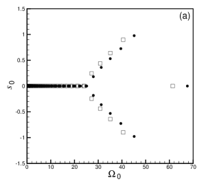
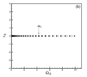
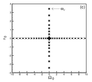
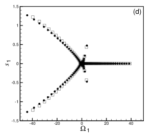
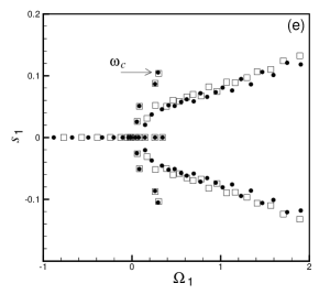
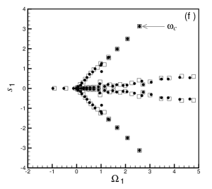
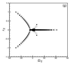
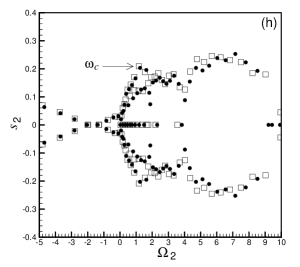
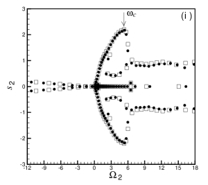
Figure 2: Eigenvalue spectra of circular discs for $\alpha=0.5$. Squares and filled circles correspond to $J$=50 and $J$=55, respectively. The converged fundamental eigenfrequency has been shown by $\omega_{c}$. Top, middle and bottom rows correspond to $m=0$, 1 and 2, respectively. Left, middle and right columns are associated with $M$=0.7, 2.5 and 5, respectively.

     

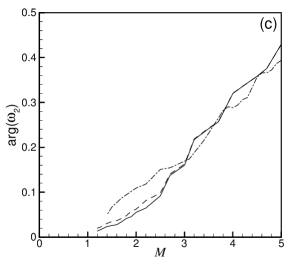
Figure 3: Variation of the fundamental eigenvalue of circular discs versus $M$. Solid, dashed and dotted lines correspond to $\alpha$=0.03, 0.1 and 0.5, respectively. (a) The growth rate $s_{0}$ of the $m=0$ mode. For this mode we have $\Omega_{0}=0$. (b) The variation of ${\rm arg}(\omega_{1})$ versus $M$. The argument of $\omega_{1}$ abruptly drops to zero at a critical $M$. This critical value tends to 1 as $\alpha$ is decreased. (c) Same as Panel b but for $m=2$. The argument of $\omega_{2}$ monotonically tends to zero by decreasing $M$.

3.2 Matrix formulation

We now substitute from (25) and (26) into (3), left-multiply both sides of the resulting equation by $-{\rm i}\hat{P}^{|k|}_{j}\textbf{W}^{-1}$ ($k=0,1,2,\cdots$), and integrate over $0\leq R<\infty$. Using the orthogonality of the associated Legendre functions, we obtain a system of linear equations for the coefficients $\hat{a}^{k}_{j}$, $\hat{b}^{k}_{j}$ and $\hat{c}^{k}_{j}$ as

$$\!\!\!\textbf{A}\cdot\textbf{X}=\frac{\omega_{m}R_{0}}{c_{0}}\textbf{X},$$ (29)

$$\!\!\!\textbf{X}^{T}=\left(\ldots,\textbf{a}_{m+n},\textbf{b}_{m+n},\textbf{c}_{m+n},\textbf{a}_{m},\textbf{b}_{m},\textbf{c}_{m},\textbf{a}_{m-n},\ldots\right),$$

$$\!\!\!\textbf{a}_{r}=\left(\hat{a}^{r}_{|r|},\hat{a}^{r}_{|r|+1},\hat{a}^{r}_{|r|+2},\ldots\right),$$

$$\!\!\!\textbf{b}_{r}=\left(\hat{b}^{r}_{|r|},\hat{b}^{r}_{|r|+1},\hat{b}^{r}_{|r|+2},\ldots\right),$$

$$\!\!\!\textbf{c}_{r}=\left(\hat{c}^{r}_{|r|},\hat{c}^{r}_{|r|+1},\hat{c}^{r}_{|r|+2},\ldots\right).$$

It is seen that $\omega_{m}R_{0}/c_{0}$ is an eigenvalue of A and X is its corresponding eigenvector. We find that the elements of A are linear combinations of the following definite integrals

$$I_{ij}^{rs}(\nu)\!\!\!\!\! = \!\!\!\!\!\int_{-1}^{1}\!\!\hat{P}^{|r|}_{i}\left(\xi\right)\left(\frac{1-\xi}{2}\right)^{\nu}\hat{P}^{|s|}_{j}\left(\xi\right)d\xi,$$

$$J_{ij}^{rs}(\nu)\!\!\!\!\! = \!\!\!\!\!\int_{-1}^{1}\!\!\hat{P}^{|r|}_{i}\left(\xi\right)\left(\frac{1+\xi}{2}\right)^{-\frac{1}{2}}\left(\frac{1-\xi}{2}\right)^{\nu}\hat{P}^{|s|}_{j}\left(\xi\right)d\xi,$$

$$K_{ij}^{rs}(\nu)\!\!\!\!\! = \!\!\!\!\!\int_{-1}^{1}\!\!\hat{P}^{|r|}_{i}\left(\xi\right)\left(\frac{1+\xi}{2}\right)^{-\frac{1}{2}}\left(\frac{1-\xi}{2}\right)^{\nu}$$

$$\!\!\!\!\times\left\{\left(\frac{1-\xi}{2}\right)+\gamma^{2}\left(\frac{1+\xi}{2}\right)\right\}^{-1}$$

$$\!\!\!\times\left\{\alpha^{2}\left(\frac{1-\xi}{2}\right)+\left(\frac{1+\xi}{2}\right)\right\}^{-1}\hat{P}^{|s|}_{j}\left(\xi\right)d\xi,$$

$$L_{ij}^{rs}(\nu)\!\!\!\!\! = \!\!\!\!\!\int_{-1}^{1}\!\!\hat{P}^{|r|}_{i}\left(\xi\right)\left(\frac{1+\xi}{2}\right)^{-\frac{1}{2}}\left(\frac{1-\xi}{2}\right)^{\nu}$$ (30)

$$\!\!\!\!\times\left\{\left(\frac{1-\xi}{2}\right)+\gamma^{2}\left(\frac{1+\xi}{2}\right)\right\}^{-2}$$

$$\!\!\!\times\left\{\alpha^{2}\left(\frac{1-\xi}{2}\right)+\left(\frac{1+\xi}{2}\right)\right\}^{-2}\hat{P}^{|s|}_{j}\left(\xi\right)d\xi,$$

where $r$ and $s$ are integer numbers of the form $m+np^{\prime}$ and $m+np^{\prime\prime}$, respectively. The integrals in (30) are evaluated using Gaussian quadratures. We transform A to Hessenberg form and obtain its corresponding QR transform (Press et al. 1997). We then compute the eigenvalues and eigenvectors of the linear system (29). Consequently, the surface density of the $m$th mode is determined from (22) and (26) as

$$\Sigma_{1,m}(R,\phi,t,\epsilon)\!\!\!\!\! = \!\!\!\!\!e^{s_{m}t}\!\!A_{m}(R,\phi,\epsilon)$$ (31)

$$\!\!\!\!\!\times\cos[m\phi\!-\!\Omega_{m}t\!+\!\Theta_{m}(R,\phi,\epsilon)],$$

$$A_{m}(R,\phi,\epsilon)\!\!\!\!\! = \!\!\!\!\!\sqrt{\Sigma^{(m)}_{1}(R,\phi,\epsilon)\bar{\Sigma}^{(m)}_{1}(R,\phi,\epsilon)},$$ (32)

$$\Theta_{m}(R,\phi,\epsilon)\!\!\!\!\! = \!\!\!\!\!\arctan\left[-{\rm i}{\Sigma^{(m)}_{1}-\bar{\Sigma}^{(m)}_{1}\over\Sigma^{(m)}_{1}+\bar{\Sigma}^{(m)}_{1}}\right]-m\phi,$$ (33)

where a bar denotes complex conjugate. One can expand $A_{m}$ and $\Theta_{m}$ in the Taylor series of $\epsilon$ as

$$Y_{m}(R,\phi,\epsilon)=Y_{m,0}(R)+\sum_{l=1}^{+\infty}\epsilon^{l}Y_{m,l}(R,\phi),~{}~{}Y\equiv(A,\Theta),$$ (34)

so that $Y_{m,l}$ are $2\pi$-periodic in $\phi$. The leading zeroth order terms of (34), $Y_{m,0}(R)$, determine the overall shape of the perturbed density, which is usually an $m$-fold trailing spiral. The higher-order terms ($l>0$) lead to density fluctuations along the major spiral arm(s).

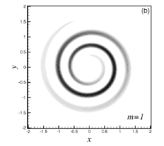
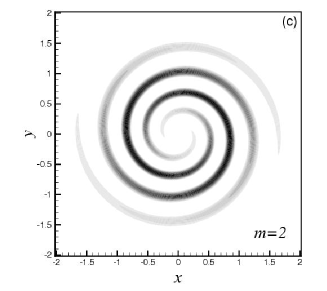
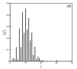
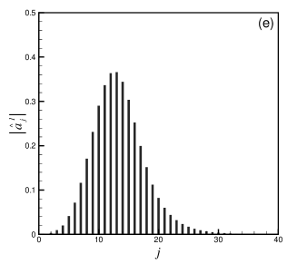
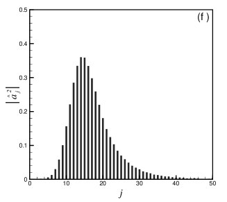
Figure 4: Top row: unstable modes of a circular disc with $\alpha=0.5$ and $M=5$. The corresponding absolute values of $\hat{a}^{m}_{j}$ ($m=0,1,2$) have been plotted versus $j$ below each mode shape. The corotation radius is $R_{\rm CR}=0.972$ and $R_{\rm CR}=0.943$ for $m=1$ and 2, respectively.

Both A and X are infinite dimensional. However, the non-axisymmetry parameter $\epsilon$ is small and its powers, which serve as the coefficients of interacting terms, fall off rapidly. Therefore, it is reasonable to truncate the series of the interacting modes in (3) at some $|l-p|=L$. We also truncate the series in (25) and (26) at $j_{\rm max}=J$. We begin with $L=1$ and $J=20$, and increase them until we acquire a relative accuracy of 1% in computing $\omega_{m}$.

In the axisymmetric limit, A becomes a block diagonal matrix and we obtain the following eigenvalue problem for the $m$th mode

$$\!\!\!\textbf{B}(m)\cdot\textbf{Z}=\frac{\omega_{m}R_{0}}{c_{0}}\textbf{Z},$$ (35)

$$\!\!\!\textbf{Z}^{T}=\left(\hat{a}^{m}_{1},\ldots,\hat{a}^{m}_{J},\hat{b}^{m}_{1},\ldots,\hat{b}^{m}_{J},\hat{c}^{m}_{1},\ldots,\hat{c}^{m}_{J}\right),$$

with $\textbf{B}(m)$ being a single $3J\times 3J$ block of A. The perturbed surface density corresponding to (35) becomes

$$\Sigma_{1,m}(R,\phi,t)=e^{s_{m}t}A_{m,0}(R)\cos\left[m\phi\!-\!\Omega_{m}t\!+\!\Theta_{m,0}(R)\right].$$ (36)

The matrix B has $3J$ eigenvalues, which lie on several branches in the complex $(\Omega_{m},s_{m})$-plane. However, eigenvalues of most branches diverge as $J$ is increased. They are virtual roots of the determinantal equation

$$\left|\textbf{B}(m)-\frac{\omega_{m}R_{0}}{c_{0}}\cdot\textbf{I}\right|=0,$$ (37)

with I being the unit matrix. Physical eigenvalues of unstable discs (if they exist) belong to a convergent complex branch. The convergent eigenvalue with the largest growth rate corresponds to the fundamental eigenmode.

The ideal scale-free limit will be attained if we let both $\alpha$ and $\gamma$ tend to zero. Our calculations show that the stability/instability properties do not change substantially by decreasing $\gamma$. The choice of $\gamma=0.05$ gives accurate and robust results in most cases. So we need to play with $\alpha$. Since the scale length of Clutton-Brock functions is fixed, by decreasing $\alpha$ we require too many terms in the expansion of $\hat{\delta}^{(k)}_{1}(R)$ to get the series converged. The smallest value of $\alpha$ that we could approach, while assuring computational accuracy, was $\alpha=0.03$.

4 Modes of circular discs

To this end, we study instabilities of cutout Mestel discs, which are obtained from the models of §2 by setting $\epsilon=0$. Calculation of unstable modes of circular discs is straightforward because the equilibrium fields do not depend on the azimuthal angle $\phi$. We set $m=0$, 1 and 2 in (35) and calculate $\omega_{m}$ over the interval $0\leq M\leq 5$. This covers all subsonic (hot) and a wide range of supersonic (cold) discs. We calculate the normal modes for $\alpha$=0.5, 0.1 and 0.03, which respectively require $J=50$, 100 and 200 for a computational accuracy of 1%.

Top row in Fig. 2 shows the eigenfrequency spectrum of the $m=0$ mode for $M$=0.7, 2.5, 5 and $\alpha=0.5$. Most eigenfrequencies of the model with $M$=0.7 are real (Fig. 2a). There are a few divergent complex eigenfrequencies whose magnitudes are increased by increasing $J$. The complex eigenfrequencies completely disappear for $1.8\mathrel{\hbox to0.0pt{\lower 3.2pt\hbox{$\sim$}\hss}\raise 1.2pt\hbox{$<$}}M\mathrel{\hbox to0.0pt{\lower 3.2pt\hbox{$\sim$}\hss}\raise 1.2pt\hbox{$<$}}2.7$ (Fig. 2b). A convergent complex branch occurs for $M>2.7$ whose eigenfrequencies correspond to non-rotating unstable ring modes with $\Omega_{m}=0$ (Fig. 2c). The fundamental eigenfrequency, denoted by $\omega_{c}$, is located at the end of the complex branch of the spectrum. Fig. 3a shows the variation of the fundamental growth rate with respect to $M$ and $\alpha$. It is seen that for $M>3$ our results do not vary that much as we change $\alpha$. The upper limit of $M$ in stable discs is $M_{\rm cr}=2.7$ for $\alpha=0.5$ and $M_{\rm cr}=2.43$ for $\alpha=0.03$. Our results for $M_{\rm cr}$ can be compared with the critical $v/\sigma$ computed from equation (6.2) of Lemos et al. (1991). Their $v$ and $\sigma$ for the $\beta=0$ models are our $V_{c}$ and $c_{0}$, respectively. By keeping the minus sign before the square root in equation (6.2) of Lemos et al. (1991) (this is to guarantee ring formation), and setting $L=1$, $\beta=0$ and $\gamma=1$, one finds $v/\sigma=2.414$. The difference between this critical number and $M_{\rm cr}=2.43$ of our $\alpha=0.03$ model is only 0.66%, which validates the accuracy of our matrix formulation based on the expansions introduced in equations (25) and (26). We note that the choice of $\alpha=0.03$ is quite enough for understanding the behavior in the scale-free limit. We have also found that unstable breathing modes do exist in subsonic discs with $\alpha=0.5$ if $M<0.56$. For $\alpha=0.03$ we find $M<0.87$, which coincides with the upper limit of $v/\sigma$ calculated in Lemos et al. (1991) for the existence of breathing modes.

The eigenfrequency spectra of the $m=1,2$ modes have three branches in the complex $(\Omega_{m},s_{m})$-plane. Subsonic discs have no convergent unstable (complex) branch. They are stable under $m=1,2$ excitations (Figs 2d and g). A continuum of convergent real eigenfrequencies exists on the $\Omega_{m}$-axis, which survives for almost all $M$, although it may be shrunk to a small interval of positive pattern speeds. Aoki et al. (1979) have encountered similar eigenfrequencies in studying the gaseous Kuzmin disc. Convergent real eigenfrequencies correspond to pure oscillatory waves. Here we are interested in growing modes and we will overlook the real branch of the spectrum. As we increase $M$, a convergent unstable branch, with the largest ${\rm arg}(\omega_{m})$=$\arctan(s_{m}/\Omega_{m})$, occurs in the spectrum. One can readily identify the fundamental eigenfrequency $\omega_{c}$ on this newly born branch. In a sufficiently cold disc, the convergent branch attracts more eigenfrequencies of the linear system (35) and ${\rm Im}(\omega_{c})$ becomes the global maximum (see Figs 2f and 2i). In Figs 3b and c we have illustrated ${\rm arg}(\omega_{m})$=$\arctan(s_{m}/\Omega_{m})$ ($m=1,2$) in terms of $M$ and for several choices of $\alpha$. These figures show that the growth rate tends to zero faster than the pattern speed while the disc is stabilized. Instabilities are suppressed in discs with $M<1$ because pressure waves travel faster than gravitationally generated waves. Figs 3b and c can be compared with Fig. 3 in GE. The graphs of ${\rm arg}(\omega_{m})$ have similar trends in our and their papers: For $m=1$, ${\rm arg}(\omega_{m})$ has a local minimum, while it is an almost monotonic function of $M$ for cold discs and for $m=2$. The major discrepancy between our and GE results occurs when $M\rightarrow 1$. GE predicted a rapid growth of ${\rm arg}(\omega_{m})$ contrary to the abrupt drop in our calculations. We ascribe the existing discrepancies to the type of imposed internal boundary conditions. We use a cutout, which disables the medium needed for the propagation of incoming waves. GE, however, fix ${\rm arg}(\omega)$ to make a reflective boundary at $R=0$.

Fig. 4 displays the unstable $m=0$, 1 and 2 modes of a circular disc with $M=5$ and $\alpha=0.5$. We have plotted the positive part of $A_{m,0}(R)\cos[m\phi+\Theta_{m,0}(R)]$. Gray scale contours mark 10 to 100 percent of the maximum perturbed density. The $m=1$ and $m=2$ modes are tightly wound spirals whose amplitude functions, $A_{1,0}(R)$ and $A_{2,0}(R)$, have only one peak. There is no local density concentration along the spiral arms and the wave amplitude slowly decays well within the corotation radius. We have also plotted $|\hat{a}^{m}_{j}|$ versus $j$ below each mode shape in Fig. 4. The plots show a rapid convergence of the sequence $|\hat{a}^{m}_{j}|$. As it can be seen in mode shapes, unstable waves cannot penetrate into the centre. This is due to the inner cutout, which damps the impinging waves by immobilizing the mass of central regions.

5 Modes of non-axisymmetric discs

We now apply the formulation of §3 and calculate the $m=0$, 1 and 2 modes of our non-axisymmetric discs. We set $L=3$, which keeps $nL+1$=7 interacting modes. Such a truncation has enough accuracy for the models with $M>1$, which mostly have $\epsilon<0.24$ (see Fig. 1). The major limiting factor in the normal mode calculation of non-axisymmetric discs is the choice of $\alpha$ whose small values need too many terms in (25) and (26) to ensure the convergency. Taking into account the fact that the size of A in non-axisymmetric discs increases by a factor of $(nL+1)\times(nL+1)$ compared to the axisymmetric limit, the run time of our eigenvalue and eigenvector solver rises drastically. To optimize the cost of numerical computations, we use $\alpha=0.5$ in our non-axisymmetric discs because it requires only $J=50$ to achieve a relative accuracy of 1%. This is a legitimate choice because according to the graphs of Fig. 3 the qualitative features of normal modes do not change by varying $\alpha$.

Fig. 5 shows the evolution of the fundamental eigenfrequencies with respect to the variations in $\epsilon$ for two choices of $M$ for each mode number $m$. Left panels in Fig. 5 correspond to a marginal $M$, which is chosen slightly larger than the upper limit of Mach number for stable circular discs. Right panels in Fig. 5 are for a cold disc with $M=5$. Left panels in Fig. 6 display the $m=0$, 1 and 2 modes of non-axisymmetric discs that bifurcate from the modes of Fig. 4. Gray scale contours show the positive part of

$$\Sigma^{(m)}_{1}(R,\phi,\epsilon)=A_{m}(R,\phi,\epsilon)\cos[m\phi+\Theta_{m}(R,\phi,\epsilon)].$$ (38)

Right panel to each mode shape shows the absolute values of the scaled expansion coefficients, $|a^{k}_{j}|$=$\epsilon^{|l|}|\hat{a}^{k}_{j}|$ ($k=m+nl$), in terms of $l$ and $j$.

   

   

   

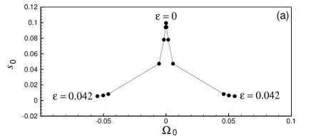
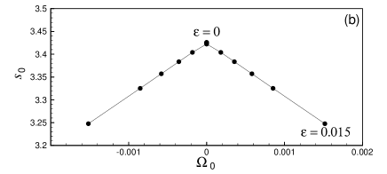
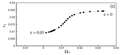
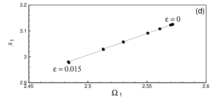
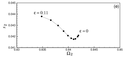
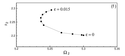
Figure 5: Evolution of the eigenfrequencies of non-axisymmetric discs with respect to $\epsilon$ and $M$. Top, middle and bottom panels correspond to $m=0$, 1 and 2, respectively. Right panels correspond to $M=5$. (a) $M$=2.8 (c) $M$=1.7 (e) $M=1.4$. As Panels a and c show, the $m=0$ and $m=1$ modes are stabilized by increasing $\epsilon$ in the allowable zone of Fig. 1. The $m=0$ mode can be stabilized for $2.7\mathrel{\hbox to0.0pt{\lower 3.2pt\hbox{$\sim$}\hss}\raise 1.2pt\hbox{$<$}}M\mathrel{\hbox to0.0pt{\lower 3.2pt\hbox{$\sim$}\hss}\raise 1.2pt\hbox{$<$}}2.91$. This interval becomes $1.6\mathrel{\hbox to0.0pt{\lower 3.2pt\hbox{$\sim$}\hss}\raise 1.2pt\hbox{$<$}}M\mathrel{\hbox to0.0pt{\lower 3.2pt\hbox{$\sim$}\hss}\raise 1.2pt\hbox{$<$}}2.3$ for $m=1$. The eigenfrequencies do not vary substantially for cold discs with $M=5$ and for the $m=2$ modes.

 

 

 

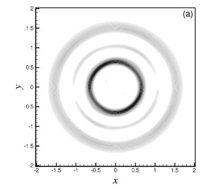
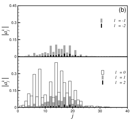
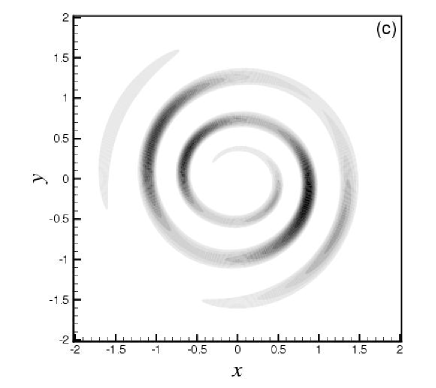
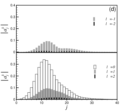
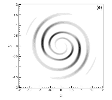
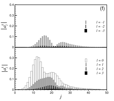
Figure 6: Mode shapes (left panels) of a set of non-axisymmetric discs with $M=5.0$ and $\alpha=0.5$. Top, middle and bottom rows correspond to $(m,\epsilon)=(0,0.015)$, (1,0.015) and (2,0.01), respectively. These modes bifurcate from the modes of Fig. 4. Gray scale contours mark 10 to 100 percent of the maximum perturbed density with a step of 10. Local density peaks (darker regions) along the major spiral arms correspond to the local maxima of $\Sigma^{(m)}_{1}(R,\phi,\epsilon)$. Right panel of each mode shape shows the corresponding absolute value of $a^{k}_{j}=\epsilon^{|l|}\hat{a}^{k}_{j}$ ($k=m+nl$) versus $j$ and $l$. The results clearly show the convergence of our perturbation series both in the radial and in the azimuthal directions.

Our computations show that non-axisymmetric discs with $M<2.7$ are stable for $m$=0 excitations independent of the magnitude of $\epsilon$. In discs with $M>2.7$ a tangent bifurcation occurs in the complex $(\Omega_{m},s_{m})$-plane at the location of each eigenfrequency (including $\omega_{c}$) and two sets of eigenfrequencies with non-zero pattern speeds come to existence. They are of the form $\omega_{0}$=$\pm\Omega_{0}+{\rm i}s_{0}$. This is an interesting result: we have found an unstable, ring-shaped density perturbation that can rotate. Our computations show that the models with $2.7\mathrel{\hbox to0.0pt{\lower 3.2pt\hbox{$\sim$}\hss}\raise 1.2pt\hbox{$<$}}M\mathrel{\hbox to0.0pt{\lower 3.2pt\hbox{$\sim$}\hss}\raise 1.2pt\hbox{$<$}}2.91$ are stabilized by increasing $\epsilon$. Fig. 5a shows that how a model with $M$=2.8 is eventually stabilized for $\epsilon\approx 0.042$. The pattern speed of the $m=0$ mode takes both positive and negative values because equation (3) is invariant under the reflections $t\rightarrow-t$ and $\phi\rightarrow-\phi$ for $m=0$. According to Fig. 1, the upper limit of $\epsilon$ decreases for our cold bisymmetric discs, and therefore, models with large $M$ cannot be stabilized only by varying the non-axisymmetry parameter. Nonetheless, the placement of eigenfrequencies in the complex plane is similar for all unstable discs: the pattern rotates faster and grows slower as $\epsilon$ increases. Fig. 6a displays the growing $m$=0 mode of a non-axisymmetric disc with $(M,\epsilon)$=$(5,0.015)$. The corresponding $|a^{m+nl}_{j}|$ (Fig. 6b) tend to zero as $|l|$ and $j$ are increased. Thus, the perturbation expansion given in (22) is convergent both in the azimuthal and in the radial directions.

Our eigenfrequency calculations for $m=1$ has been summarized in Figs 5c and d for $M=$1.7 and $5$, respectively. The unstable $m=1$ mode has a definite sense of rotation and its pattern speed decreases as $\epsilon$ is increased. For the disc with $M=1.7$, $\omega_{m}$ steeply falls off and ultimately vanishes for $\epsilon\approx 0.05$. This property is shared by all models in the range $1.6\mathrel{\hbox to0.0pt{\lower 3.2pt\hbox{$\sim$}\hss}\raise 1.2pt\hbox{$<$}}M\mathrel{\hbox to0.0pt{\lower 3.2pt\hbox{$\sim$}\hss}\raise 1.2pt\hbox{$<$}}2.3$. Models with $M<1.6$ are stable for $m=1$ excitations regardless of the magnitude of $\epsilon$. The fundamental eigenfrequency of the models with $M>2.3$ does not vary considerably as $\epsilon$ is increased in the admissible zone of Fig. 1. However, the mode shape is highly influenced by the non-axisymmetry. Fig. 6c shows the unstable $m=1$ mode of a non-axisymmetric disc with $(M,\epsilon)$=$(5,0.015)$. Although the overall shape is a single armed spiral, which corresponds to the $l=0$ wave component of equation (14), a number of dense clumps occur along the major spiral arm. These local clumps are generated by the $|l|>0$ wave components of the perturbed density expansion. Fig. 6d shows the variation of $|a^{m+nl}_{j}|$ versus $l$ and $j$ for $m=1$. The sequence nicely converges as $|l|$ is increased. It is seen that the choice of $L=2$ provides enough accuracy both for $m=0$ and for $m=1$.

Finding the eigenfrequencies of the $m=2$ mode for $M<2$ is troublesome because the convergent complex branch emerges very close to divergent branches (see Fig. 2h). We have written a program that computes the full eigenvalue spectrum for several choices of $J$ and searches between all eigenvalues for the most convergent one. According to our program, convergent unstable $m=2$ modes exist for $M\geq 1.4$. Numerical results displayed in Fig. 5e and f show that the fundamental eigenfrequency is robust to variations in $\epsilon$. The corresponding mode shapes are double armed spirals with some sort of dense clumps distributed along the major arms. The pitch angle of the global arms deceases as the disc is cooled (large $M$). Fig. 6e displays the $m=2$ mode of a non-axisymmetric disc with $(M,\epsilon)$=$(5,0.01)$. The perturbation series (22) slowly converges in the $\phi$-direction for $m=2$. So we kept more azimuthal wave components and used $L=3$ (Fig. 6f).

6 Discussions

The classical procedure in the instability analysis of gaseous (and stellar) discs is to start with an axisymmetric equilibrium and then perturb the governing equations in the vicinity of this equilibrium state. The subsequent eigenvalue problem [e.g., equation (35)] results in a complex frequency $\omega_{m}=\Omega_{m}+{\rm i}s_{m}$, which implies an $m$-fold barred/spiral pattern $\Sigma_{m}=A_{m}(R)\cos[m\phi+\Theta_{m}(R)]$ that rotates by the angular velocity $\Omega_{m}/m$ and exponentially grows by the rate $s_{m}$. Nevertheless, most events of physical significance happen in nonlinear regime when the modes begin to interact. In such a circumstance, more than one azimuthal wave component is present in the response spectrum. The most general form of a density wave in nonlinear regime is

$$\Sigma_{1}(R,\phi,t)=\sum_{m=-\infty}^{+\infty}A_{m}(R,t)e^{{\rm i}[m\phi+\Theta_{m}(R,t)]},$$ (39)

which means that the amplitude and phase angle of $\Sigma_{1}$ are functions of all spatial and time variables. A primary result of (39) is the generation of dense clumps at the locations of the maxima of $\Sigma_{1}$. Clumps may undergo gravitational collapse, merge and give birth to gas giants. This is a widely accepted formation scenario of protoplanets (e.g., Boss 1997; Mayer et al. 2004) because it can take place in short time scales. Asymmetries like the presence of a double star (Boss 2006) can also generate dense clumps.

According to (31) and calculations of §5, unstable density waves of non-axisymmetric discs have a rich structure (in linear regime) even for very small non-axisymmetry parameter $\epsilon$. Although the temporal evolution of the $m$th mode is governed by the simple function $\exp({\rm i}\omega_{m}t)$, the eigenfunction associated with $\omega_{m}$ is by no means simple and it contains infinite number of azimuthal wave components, which in turn are capable of generating local clumps. Since realistic accretion discs have not initially the nice axisymmetry feature, their instability can give birth to protoplanets sooner than what nonlinear hydrodynamical simulations predict. A protoplanet, as a possible product of the gravitational collapse of a dense clump, is separated from the rest of the evolving gas and migrates until it is captured by a resonant island in the phase space.

Our perturbation theory can be applied to any non-axisymmetric configuration regardless of the nature of the centre. Cutouts, which are special treatments designed for scale-free models, are not needed in cored systems with finite total mass. The most important factor in success of our perturbation theory is the smallness of the non-axisymmetry parameter $\epsilon$, which prohibits the interaction of azimuthal wave components in the zeroth order terms. Our equilibrium density has a single azimuthal Fourier component [see equation (3)]. Accordingly, the harmonic numbers of wave components differ in steps of $nl$ ($l=0,\pm 1,\pm 2,\cdots$). For bisymmetric discs studied in this paper, this means that wave components have only even or odd harmonic numbers. We will have the most complete spectrum if the equilibrium fields include Fourier terms with both even and odd harmonic numbers, or if the disc is lopsided with $n=1$.

We presented three length scales to the perturbed equation (14). The first two are the cutout radii, $R_{\rm in}$ and $R_{\rm out}$, and the third one is the length scale of the basis functions, $R_{C}$. At a first look, such a treatment of scale-free systems seems unfavorable because in this way we destroy their scale-invariance and cuspy features. However, with appropriate selection of the exponents of the cutout functions, $N_{\rm in}$=$N_{\rm out}$=2, and the weight function of the velocity components, $w_{2}(\xi)$, the coefficient matrix A of our eigenvalue problem became a function of the two dimensionless parameters $\alpha$ and $\gamma$. We easily decreased $\gamma$ and noticed that unstable waves do not extend to distant regions although the mass of our equilibrium models (with flat rotation curves) is infinite at $R\rightarrow\infty$. We then let $\alpha$ tend to zero with the aim of removing the inner cutout. This needed more terms of the series of associated Legendre functions, but the qualitative features of our results remained unchanged as long as mode shapes and ${\rm arg}(\omega_{m})$ were concerned. There was an excellent match between our results and those of Lemos et al. (1991) who used logarithmic spirals to model their perturbed quantities. Logarithmic spirals do not introduce any length scale to variational equations.

The critical value of $M$, below which our bisymmetric discs are stable, is a function of the fundamental wave number $m$. Numerical results show that the models with $\alpha=0.5$ are stable for $m=0$ excitations when $M\mathrel{\hbox to0.0pt{\lower 3.2pt\hbox{$\sim$}\hss}\raise 1.2pt\hbox{$<$}}2.7$. This limit approximately becomes $1.6$ and $1.4$ for $m=1$ and 2, respectively. The most interesting property that we have found for unstable non-axisymmetric discs is that the $m=0$ and $m=1$ modes can be stabilized by increasing the non-axisymmetry parameter $\epsilon$. This happens for $m=0$ when $2.7\mathrel{\hbox to0.0pt{\lower 3.2pt\hbox{$\sim$}\hss}\raise 1.2pt\hbox{$<$}}M\mathrel{\hbox to0.0pt{\lower 3.2pt\hbox{$\sim$}\hss}\raise 1.2pt\hbox{$<$}}2.91$ and for $m=1$ when $1.6\mathrel{\hbox to0.0pt{\lower 3.2pt\hbox{$\sim$}\hss}\raise 1.2pt\hbox{$<$}}M\mathrel{\hbox to0.0pt{\lower 3.2pt\hbox{$\sim$}\hss}\raise 1.2pt\hbox{$<$}}2.3$. There are some remarkable differences between the stabilized $m=0$ and $m=1$ modes. The stabilized $m=0$ mode has the form of a ring, which rotates according to the results displayed in Fig. 5a. It occurs when the wave components with the azimuthal harmonic numbers $m-nl=-nl$ and $m+nl=nl$ cancel each other for $l>0$. The stabilized $m=1$ mode, however, is a non-spiral, equiangular neutral mode. It emerges for a sufficiently large $\epsilon$, when the wave component with the harmonic number $m-n=-1$ ($l=-1$) cancels the fundamental component with $m+n\times 0=1$ ($l=0$). It is worth noting that the $m=2$ mode cannot be stabilized by increasing $\epsilon$, because the interacting wave components of ${\cal O}(\epsilon)$ have the harmonic numbers $m-n=0$ ($l=-1$) and $m+n=4$ ($l=1$). Neither of these first-order components is capable of suppressing the effect of the fundamental component with the harmonic number $m+n\times 0=2$. On the other hand, the wave component with the harmonic number $m-n\times 2=-2$ is of ${\cal O}(\epsilon^{2})$, which is too weak to compensate the zeroth order $m=2$ component. Based on the above reasonings, we speculate that the $m=2$ mode can be stabilized in discs whose surface density includes the fourth harmonic of the azimuthal angle or when $n=4$ in the simple discs of JA. Furthermore, the unstable $m=1$ and $m=2$ modes of lopsided discs (with $n=1$) cannot be stabilized by increasing the non-axisymmetry parameter.

7 Acknowledgments

During the first 2 years of his PhD program, NMA received a research grant from the Aerospace Research Institute through a collaboration scheme between the IASBS and ARI. NMA also thanks Prof. Mohsen Bahrami for insightful discussions.

Appendix A The elements of the Linear operator ${\bf L}$

The linear operator ${\bf L}$ appeared in equation (17) is in terms of the active surface density $\Sigma_{\rm act}(R,\phi)$, and the velocity field

$$\left(u_{20},u_{30}\right)$=$\left[v_{R0}(R,\phi),v_{\phi 0}(R,\phi)\right],$$ (40)

of the equilibrium state. The elements of ${\bf L}$ are

$$L_{11}\!\!\!\! = \!\!\!\!{1\over\Sigma_{\rm act}}\bigg{(}{\partial_{t}}+{v_{R0}\over R}+v_{R0}\partial_{R}+{v_{\phi 0}\over R}\partial_{\phi}$$ (41)

$$\!\!\!\!\qquad\qquad+\partial_{R}v_{R0}+{\partial_{\phi}v_{\phi 0}\over R}\bigg{)},$$

$$L_{12}\!\!\!\! = \!\!\!\!{1\over R}+\left[\partial_{R}+\partial_{R}\left(\ln\Sigma_{\rm act}\right)\right],$$ (42)

$$L_{13}\!\!\!\! = \!\!\!\!{1\over R}\left[\partial_{\phi}+\partial_{\phi}\left(\ln\Sigma_{\rm act}\right)\right],$$ (43)

$$L_{21}\!\!\!\! = \!\!\!\!{c^{2}(\phi)\over\Sigma_{\rm act}}\left[\partial_{R}-\partial_{R}\left(\ln\Sigma_{\rm act}\right)\right],$$ (44)

$$L_{22}\!\!\!\! = \!\!\!\!{\partial_{t}}+\partial_{R}v_{R0}+v_{R0}\partial_{R}+{v_{\phi 0}\over R}\partial_{\phi},$$ (45)

$$L_{23}\!\!\!\! = \!\!\!\!{1\over R}\partial_{\phi}v_{R0}-{2v_{\phi 0}\over R},$$ (46)

$$L_{31}\!\!\!\! = \!\!\!\!{1\over\Sigma_{\rm act}}\left\{\frac{1}{R}\partial_{\phi}c^{2}(\phi)+{c^{2}(\phi)\over R}\left[\partial_{\phi}-\partial_{\phi}\left(\ln\Sigma_{\rm act}\right)\right]\right\},$$ (47)

$$L_{32}\!\!\!\! = \!\!\!\!\partial_{R}v_{\phi 0}+{v_{\phi 0}\over R},$$ (48)

$$L_{33}\!\!\!\! = \!\!\!\!{\partial_{t}}+\frac{1}{R}\partial_{\phi}v_{\phi 0}+{v_{R0}\over R}+v_{R0}\partial_{R}+{v_{\phi 0}\over R}\partial_{\phi}.$$ (49)

Appendix B The elements of the operator matrices $\textbf{D}_{p}$

The operators ${\textbf{D}}_{p}$=$[D_{p,ij}]$ ($i,j=1,2,3$) appear in the interacting terms of (3). They are functions of $R$ and ${\rm d}/{\rm d}R$. Let us define $k=m+nl$ and introduce

$$\!\!\!H(R)=\frac{R^{2}}{R^{2}+\alpha^{2}R_{0}^{2}}\ \frac{R_{0}^{2}}{\gamma^{2}R^{2}+R_{0}^{2}},$$

$$\!\!\!H_{1}(R)=1+\alpha^{2}\gamma^{2}+3\gamma^{2}\left(\frac{R}{R_{0}}\right)^{2}-\alpha^{2}\left(\frac{R_{0}}{R}\right)^{2},$$

$$\!\!\!\mu_{1}=1-\left[\frac{5M^{2}-1+3n(M^{2}-1)}{2(1+n)}\right]\epsilon^{2},$$

$$\!\!\!\mu_{2}=\frac{4+3\epsilon^{2}+8n(1-2n)\left(1+\epsilon^{2}\right)}{8(1+n)(-1+4n^{2})}$$

$$\!\!\!-\frac{16n^{3}\left(2+3\epsilon^{2}\right)}{8(1+n)(-1+4n^{2})}$$

$$\!\!\!+M^{2}\left[\frac{2+n}{2(1+n)}+\frac{72n^{3}+104n^{2}-22n-27}{8(1+n)(-1+4n^{2})}\ \epsilon^{2}\right],$$

$$\!\!\!\mu_{3}=\frac{12n^{3}+6n^{2}-n-1}{4(1+n)(-1+4n^{2})}$$

$$\!\!\!-M^{2}\frac{12n^{3}+18n^{2}-5n-5}{4(1+n)(-1+4n^{2})},$$

$$\!\!\!\mu_{4}=\frac{-16n^{3}-8n^{2}+1}{8(1+n)(-1+4n^{2})}$$

$$\!\!\!+M^{2}\frac{24n^{3}+32n^{2}-10n-9}{8(1+n)(-1+4n^{2})}.$$

For $|p|\leq 3$, we have found

$$D_{0,11}\!\!\! = \!\!\!\textrm{i}kM\left(\frac{R_{0}}{R}\right)\left(1+\frac{1}{2}\epsilon^{2}\right),$$

$$D_{0,12}\!\!\! = \!\!\!2H^{2}(R)\left[\alpha^{2}\left(\frac{R_{0}}{R}\right)^{4}-\gamma^{2}\right]$$

$$\!\!\!+H(R)\left(\frac{R_{0}^{2}}{R}\right)\frac{d}{dR},$$

$$D_{0,13}\!\!\! = \!\!\!\textrm{i}kH(R)\left(\frac{R_{0}}{R}\right)^{2},$$

$$D_{0,21}\!\!\! = \!\!\!\mu_{1}H_{1}(R)+\mu_{1}\frac{R}{H(R)}\frac{d}{dR},$$

$$D_{0,22}\!\!\! = \!\!\!\textrm{i}kM\left(\frac{R_{0}}{R}\right)\left(1+\frac{1}{2}\epsilon^{2}\right),$$

$$D_{0,23}\!\!\! = \!\!\!-2M\left(\frac{R_{0}}{R}\right)\left(1+\frac{1}{2}\epsilon^{2}\right),$$

$$D_{0,31}\!\!\! = \!\!\!\textrm{i}k\mu_{1}\frac{1}{H(R)},$$

$$D_{0,32}\!\!\! = \!\!\!M\left(\frac{R_{0}}{R}\right)\left(1+\frac{1}{2}\epsilon^{2}\right),$$

$$D_{0,33}\!\!\! = \!\!\!\textrm{i}kM\left(\frac{R_{0}}{R}\right)\left(1+\frac{1}{2}\epsilon^{2}\right),$$

$$D_{+1,11}\!\!\! = \!\!\!-\textrm{i}\frac{1+M^{2}}{2M(1+n)}$$

$$\!\!\!\times\left[H_{1}(R)H(R)\left(\frac{R_{0}}{R}\right)+R_{0}\frac{d}{dR}\right]$$

$$\!\!\!-\textrm{i}kM\left(\frac{1}{2}+\frac{3}{8}\epsilon^{2}\right)\left(\frac{R_{0}}{R}\right),$$

$$D_{+1,12}\!\!\! = \!\!\!H^{2}(R)\left[\alpha^{2}\left(\frac{R_{0}}{R}\right)^{4}-\gamma^{2}\right]$$

$$\!\!\!+\frac{1}{2}H(R)\left(\frac{R_{0}^{2}}{R}\right)\frac{d}{dR},$$

$$D_{+1,13}\!\!\! = \!\!\!\frac{1}{2}\textrm{i}kH(R)\left(\frac{R_{0}}{R}\right)^{2},$$

$$D_{+1,21}\!\!\! = \!\!\!\mu_{2}H_{1}(R)+\mu_{2}\frac{R}{H(R)}\frac{d}{dR},$$

$$D_{+1,22}\!\!\! = \!\!\!-\textrm{i}\frac{1+M^{2}}{2M(1+n)}R_{0}\frac{d}{dR}$$

$$\!\!\!-\textrm{i}M(k+n)\left(\frac{1}{2}+\frac{3}{8}\epsilon^{2}\right)\left(\frac{R_{0}}{R}\right),$$

$$D_{+1,23}\!\!\! = \!\!\!\left[\frac{M^{2}(2+n)-n}{2M(1+n)}+\frac{3}{4}M\epsilon^{2}\right]\left(\frac{R_{0}}{R}\right),$$

$$D_{+1,31}\!\!\! = \!\!\!\textrm{i}k\mu_{2}\frac{1}{H(R)},$$

$$D_{+1,32}\!\!\! = \!\!\!-M\left(\frac{1}{2}+\frac{3}{8}\epsilon^{2}\right)\left(\frac{R_{0}}{R}\right),$$

$$D_{+1,33}\!\!\! = \!\!\!-\textrm{i}\frac{1+M^{2}}{2M(1+n)}\left[R_{0}\frac{d}{dR}+\left(\frac{R_{0}}{R}\right)\right]$$

$$\!\!\!-\textrm{i}kM\left(\frac{1}{2}+\frac{3}{8}\epsilon^{2}\right)\left(\frac{R_{0}}{R}\right),$$

$$D_{-1,11}\!\!\! = \!\!\!\textrm{i}\frac{1+M^{2}}{2M(1+n)}$$

$$\!\!\!\times\left[H_{1}(R)H(R)\left(\frac{R_{0}}{R}\right)+R_{0}\frac{d}{dR}\right]$$

$$\!\!\!-\textrm{i}kM\left(\frac{1}{2}+\frac{3}{8}\epsilon^{2}\right)\left(\frac{R_{0}}{R}\right),$$

$$D_{-1,12}\!\!\! = \!\!\!H^{2}(R)\left[\alpha^{2}\left(\frac{R_{0}}{R}\right)^{4}-\gamma^{2}\right]$$

$$\!\!\!+\frac{1}{2}H(R)\left(\frac{R_{0}^{2}}{R}\right)\frac{d}{dR},$$

$$D_{-1,13}\!\!\! = \!\!\!\frac{1}{2}\textrm{i}kH(R)\left(\frac{R_{0}}{R}\right)^{2},$$

$$D_{-1,21}\!\!\! = \!\!\!\mu_{2}H_{1}(R)+\mu_{2}\frac{R}{H(R)}\frac{d}{dR},$$

$$D_{-1,22}\!\!\! = \!\!\!\textrm{i}\frac{1+M^{2}}{2M(1+n)}R_{0}\frac{d}{dR}$$

$$\!\!\!-\textrm{i}M(k-n)\left(\frac{1}{2}+\frac{3}{8}\epsilon^{2}\right)\left(\frac{R_{0}}{R}\right),$$

$$D_{-1,23}\!\!\! = \!\!\!\left[\frac{M^{2}(2+n)-n}{2M(1+n)}+\frac{3}{4}M\epsilon^{2}\right]\left(\frac{R_{0}}{R}\right),$$

$$D_{-1,31}\!\!\! = \!\!\!\textrm{i}k\mu_{2}\frac{1}{H(R)},$$

$$D_{-1,32}\!\!\! = \!\!\!-M\left(\frac{1}{2}+\frac{3}{8}\epsilon^{2}\right)\left(\frac{R_{0}}{R}\right)$$

$$D_{-1,33}\!\!\! = \!\!\!\textrm{i}\frac{1+M^{2}}{2M(1+n)}\left[R_{0}\frac{d}{dR}+\left(\frac{R_{0}}{R}\right)\right]$$

$$\!\!\!-\textrm{i}kM\left(\frac{1}{2}+\frac{3}{8}\epsilon^{2}\right)\left(\frac{R_{0}}{R}\right),$$

$$D_{+2,11}\!\!\! = \!\!\!\textrm{i}\frac{1+M^{2}}{4M(-1+4n^{2})}$$

$$\!\!\!\times\left[H_{1}(R)H(R)\left(\frac{R_{0}}{R}\right)+R_{0}\frac{d}{dR}\right]$$

$$\!\!\!+\frac{1}{4}\textrm{i}kM\left(\frac{R_{0}}{R}\right),$$

$$D_{+2,12}\!\!\! = \!\!\!0$$

$$D_{+2,13}\!\!\! = \!\!\!0$$

$$D_{+2,21}\!\!\! = \!\!\!\mu_{3}H_{1}(R)+\mu_{3}\frac{R}{H(R)}\frac{d}{dR}$$

$$D_{+2,22}\!\!\! = \!\!\!\textrm{i}\frac{1+M^{2}}{4M(-1+4n^{2})}R_{0}\frac{d}{dR}$$

$$\!\!\!+\textrm{i}\frac{M(k+2n)}{4}\left(\frac{R_{0}}{R}\right)$$

$$D_{+2,23}\!\!\! = \!\!\!\frac{n+M^{2}(1+n-4n^{2})}{2M(-1+4n^{2})}\left(\frac{R_{0}}{R}\right)$$

$$D_{+2,31}\!\!\! = \!\!\!\textrm{i}k\mu_{3}\frac{1}{H(R)}$$

$$D_{+2,32}\!\!\! = \!\!\!\frac{1}{4}M\left(\frac{R_{0}}{R}\right)$$

$$D_{+2,33}\!\!\! = \!\!\!\textrm{i}\frac{1+M^{2}}{4M(-1+4n^{2})}\left[\left(\frac{R_{0}}{R}\right)+R_{0}\frac{d}{dR}\right]$$

$$\!\!\!+\frac{1}{4}\textrm{i}kM\left(\frac{R_{0}}{R}\right)$$

$$D_{-2,11}\!\!\! = \!\!\!-\textrm{i}\frac{1+M^{2}}{4M(-1+4n^{2})}$$

$$\!\!\!\times\left[H_{1}(R)H(R)\left(\frac{R_{0}}{R}\right)+R_{0}\frac{d}{dR}\right]$$

$$\!\!\!+\frac{1}{4}\textrm{i}kM\left(\frac{R_{0}}{R}\right),$$

$$D_{-2,12}\!\!\! = \!\!\!0,$$

$$D_{-2,13}\!\!\! = \!\!\!0,$$

$$D_{-2,21}\!\!\! = \!\!\!\mu_{3}H_{1}(R)+\mu_{3}\frac{R}{H(R)}\frac{d}{dR},$$

$$D_{-2,22}\!\!\! = \!\!\!-\textrm{i}\frac{1+M^{2}}{4M(-1+4n^{2})}R_{0}\frac{d}{dR}$$

$$\!\!\!+\textrm{i}\frac{M(k-2n)}{4}\left(\frac{R_{0}}{R}\right),$$

$$D_{-2,23}\!\!\! = \!\!\!\frac{n+M^{2}(1+n-4n^{2})}{2M(-1+4n^{2})}\left(\frac{R_{0}}{R}\right),$$

$$D_{-2,31}\!\!\! = \!\!\!\textrm{i}k\mu_{3}\frac{1}{H(R)},$$

$$D_{-2,32}\!\!\! = \!\!\!\frac{1}{4}M\left(\frac{R_{0}}{R}\right),$$

$$D_{-2,33}\!\!\! = \!\!\!-\textrm{i}\frac{1+M^{2}}{4M(-1+4n^{2})}\left[\left(\frac{R_{0}}{R}\right)+R_{0}\frac{d}{dR}\right]$$

$$\!\!\!+\frac{1}{4}\textrm{i}kM\left(\frac{R_{0}}{R}\right),$$

$$D_{+3,11}\!\!\! = \!\!\!-\frac{1}{8}\textrm{i}kM\left(\frac{R_{0}}{R}\right),$$

$$D_{+3,12}\!\!\! = \!\!\!0,$$

$$D_{+3,13}\!\!\! = \!\!\!0,$$

$$D_{+3,21}\!\!\! = \!\!\!\mu_{4}H_{1}(R)+\mu_{4}\frac{R}{H(R)}\frac{d}{dR},$$

$$D_{+3,22}\!\!\! = \!\!\!-\frac{1}{8}\textrm{i}M(k+3n)\left(\frac{R_{0}}{R}\right),$$

$$D_{+3,23}\!\!\! = \!\!\!\frac{1}{4}M\left(\frac{R_{0}}{R}\right),$$

$$D_{+3,31}\!\!\! = \!\!\!\textrm{i}k\mu_{4}\frac{1}{H(R)},$$

$$D_{+3,32}\!\!\! = \!\!\!-\frac{1}{8}M\left(\frac{R_{0}}{R}\right),$$

$$D_{+3,33}\!\!\! = \!\!\!-\frac{1}{8}\textrm{i}kM\left(\frac{R_{0}}{R}\right),$$

$$D_{-3,11}\!\!\! = \!\!\!-\frac{1}{8}\textrm{i}kM\left(\frac{R_{0}}{R}\right),$$

$$D_{-3,12}\!\!\! = \!\!\!0,$$

$$D_{-3,13}\!\!\! = \!\!\!0,$$

$$D_{-3,21}\!\!\! = \!\!\!\mu_{4}H_{1}(R)+\mu_{4}\frac{R}{H(R)}\frac{d}{dR},$$

$$D_{-3,22}\!\!\! = \!\!\!-\frac{1}{8}\textrm{i}M(k-3n)\left(\frac{R_{0}}{R}\right),$$

$$D_{-3,23}\!\!\! = \!\!\!\frac{1}{4}M\left(\frac{R_{0}}{R}\right),$$

$$D_{-3,31}\!\!\! = \!\!\!\textrm{i}k\mu_{4}\frac{1}{H(R)},$$

$$D_{-3,32}\!\!\! = \!\!\!-\frac{1}{8}M\left(\frac{R_{0}}{R}\right),$$

$$D_{-3,33}\!\!\! = \!\!\!-\frac{1}{8}\textrm{i}kM\left(\frac{R_{0}}{R}\right).$$

References

- [Aoki & Iye 1978] Aoki S., Iye M. 1978, PASJ, 30, 519
- [Aoki, Noguchi & Iye 1979] Aoki S., Noguchi M., Iye M. 1979, PASJ, 31, 737
- [Binney & Tremaine1987] Binney J., Tremaine S., 1987, Galactic Dynamics, Princeton University Press, Princeton
- [Boss1997] Boss A.P., 1997, Science, 276, 1836
- [Boss2006] Boss A.P., 2006, ApJ, 641, 1148
- [Clutton-Brock 1972] Clutton-Brock M., 1972, Ap&SS, 16, 101
- [Evans & Read1998a] Evans N.W., Read J.C.A., 1998a, MNRAS, 300, 83
- [Evans & Read1998b] Evans N.W., Read J.C.A., 1998b, MNRAS, 300, 106
- [Galli et al.2001] Galli D., Shu F.H., Laughlin G., Lizano S., 2001, ApJ, 551, 367
- [Goodman & Evans1999] Goodman J., Evans N.W., 1999, MNRAS, 309, 599 (GE)
- [Hunter1963] Hunter C., 1963, MNRAS, 126, 299
- [Jalali & Abolghasemi2002] Jalali M.A., Abolghasemi M., 2002, ApJ, 580, 718 (JA)
- [Kuzmin1956] Kuzmin G.G., 1956, Astr. Zh., 33, 27
- [Lemos et al.1991] Lemos J.P.S., Kalnajs A.J., Lynden-Bell D., 1991, ApJ, 375, 484
- [Mayer et al.2004] Mayer L., Quinn T., Wadsley J., Stadel J. 2004, ApJ, 609, 1045
- [Mestel1963] Mestel L., 1963, MNRAS, 126, 553
- [Papaloizou & Lin1989] Papaloizou J.C., Lin D.N.C., 1989, ApJ, 344, 645
- [Papaloizou & Savonije1991] Papaloizou J.C., Savonije G.J., 1991, MNRAS, 248, 353
- [Press et al.1997] Press W.H., Teukolsky S.A., Vetterling W.T., Flannery B.P. 1997, Numerical Recipes in C 2nd ed., Cambridge University Press, Cambridge
- [Savonije & Heemskerk1990] Savonije G.J., Heemskerk M.H.M., 1990, A&A, 240, 191
- [Syer & Tremaine1996] Syer D., Tremaine S., 1996, MNRAS, 281,925
- [Zang1976] Zang T.A., 1976, Ph.D thesis, Massachusetts Institute of Technology