Production of Hypervelocity Stars through Encounters with Stellar-Mass Black Holes in the Galactic Centre

Abstract

Stars within 0.1 pc of the supermassive black hole Sgr A* at the Galactic centre are expected to encounter a cluster of stellar-mass black holes (BHs) that have segregated to that region. Some of these stars will scatter off an orbiting BH and be kicked out of the Galactic centre with velocities up to $\sim\,2000\,$${\rm km\,s}^{-1}$. We calculate the resulting ejection rate of hypervelocity stars (HVSs) by this process under a variety of assumptions, and find it to be comparable to the tidal disruption rate of binary stars by Sgr A*, first discussed by Hills (1988). Under some conditions, this novel process is sufficient to account for all of the hypervelocity B-stars observed in the halo, and may dominate the production rate of all HVSs with lifetimes much less than the relaxation time-scale at a distance $\sim 2\,$pc from Sgr A* ($\gtrsim 2\,$Gyr). Since HVSs are produced by at least two unavoidable processes, the statistics of HVSs could reveal bimodal velocity and mass distributions, and can constrain the distribution of BHs and stars in the innermost $0.1\,$pc around Sgr A*.

1 Introduction

Hypervelocity stars (HVSs) have velocities so great ($\sim 1000\,$${\rm km\,s}^{-1}$) that they are gravitationally unbound to the Milky Way galaxy. Since the discovery of the first HVS by Brown et al. (2005), six additional HVSs have been found (Edelmann et al., 2005; Hirsch et al., 2005; Brown et al., 2006a, b). The age and radial velocities of all but one HVS are consistent with them originating from the Galactic centre, the most natural site for producing them (Hills 1988). As more HVSs are found, they can be used to constrain many properties of both the Galactic centre as well as the Milky-Way galaxy as a whole, providing information about the Galactic potential (Gnedin et al., 2005; Bromley et al., 2006), the merger history of the Sgr A* (Levin, 2005; Baumgardt et al., 2006), as well as the mass distribution of stars near Sgr A*.

Nearly 17 years before the initial discovery by Brown et al. (2005), Hills (1988) first proposed that HVSs should populate the galaxy and provide indirect evidence for the existence of a supermassive black hole (SMBH) in the Galactic centre. Hills (1988) showed that when a tight stellar binary (with a separation $<0.1\,$AU) gets sufficiently close to a SMBH, it will be disrupted by its strong tidal field. Consequently, one member of the binary could be ejected from the Galactic centre with sufficient energy to escape the gravitational potential of the entire galaxy (Hills, 1991; Gualandris et al., 2005). The other binary member is expected to remain in a highly eccentric orbit around the SMBH (see, e.g., Gould & Quillen, 2003; Ginsburg & Loeb, 2006). Yu & Tremaine (2003) analysed the production rate of HVSs in more detail, specifically for stars originating near the SMBH in our galaxy, Sgr A*. The authors also corrected the initial calculation of Hills (1988) and accounted for the diffusion of hard binaries into the “loss–cone”, finding the production rate of HVSs to be $\sim\,10^{-5}\,$yr^-1, nearly three orders of magnitude below the previous estimate. Yu & Tremaine (2003) also looked at two additional mechanisms for producing HVSs. They found that the rate could easily be higher ($\sim\,10^{-4}\,$yr^-1) if Sgr A* had a massive binary companion (see also Levin, 2005; Baumgardt et al., 2006; Sesana et al., 2006), and also determined that star-star scattering near Sgr A* resulted in a nearly undetectable rate, due to physical collisions among the two stars.

In examining the rate estimate from Yu & Tremaine (2003)  one may adopt a simple mass function (MF) for stars, ${\rm d}n/{\rm d}m\propto m^{-\beta}$ to estimate the total number of B–type HVSs in the Galactic halo. Using the Salpeter MF slope $\beta=2.35$ and a minimum mass limit of $0.5\,M_{\odot}$ one expects there to be about $\sim\,80$ HVSs with masses between $3$ and $5\,M_{\odot}$, consistent with the observed rate for such stars (Brown et al., 2006a). However this is an overestimate. The Salpeter MF overestimates the total number of stars with mass $>\,3\,M_{\odot}$, since star formation occurs continuously over time near the Galactic centre and massive stars have short lifetimes (Alexander & Sternberg, 1999; Perets et al., 2006). Accounting for continuous star formation as well as a more realistic distribution of binary parameters, Perets et al. (2006) found a lower total HVS rate of $5\times 10^{-7}\,$yr^-1 yielding $\sim 1$ HVS in the entire galaxy with mass between $3$ and $5\,M_{\odot}$. The discrepancy between this calculation and the number of observed HVSs may be overcome by massive perturbers in the Galactic centre, which reduce the relaxation time and increase the rate to that observed (Perets et al., 2006). Nevertheless, their results are highly sensitive to the mass distribution of the perturbers. In their calculations the authors use a very flat slope for the distribution of masses which has not been well constrained by observations. In their estimate, they assume that all stars are initially relaxed and therefore fill the entire energy-momentum space. The lifetimes of the stars observed by Brown et al. (2006a) are very similar to the enhanced relaxation time, except in the most optimistic case of Perets et al. (2006). We argue then that the total number of B-type HVSs given by Perets et al. (2006) may still be an overestimate, and an additional source of HVSs may be required.

In this paper, we propose a novel source of HVSs in the Milky Way: in the dense stellar cusp near Sgr A*  stars scatter off stellar-mass black holes (BHs) that are segregated there (Morris, 1993) and recoil out of the Galactic centre. The existence of stars on radial orbits originating from the Galactic centre was first proposed by Miralda-Escudé & Gould (2000) as evidence for a segregated BH cluster. Here, we show that there should exist a high-velocity tail of stars, significant enough in number to account for some if not all of the HVSs observed by Brown et al. (2006a).

This paper is organised as follows. In §2 we describe the distribution of stars and BHs around Sgr A*. We describe in detail our assumptions and calculations in §3, and present our results in §4. Finally, in §5, we discuss the observational implications and prospects for future work.

2 The cusp of stars and BHs around Sgr A*

Using near-infrared adaptive optics imaging, Genzel et al. (2003) showed that the density of stars in the innermost $\sim 2\,$pc of the Galactic centre is well-fit by a broken power-law radial profile, $\rho(R)=1.2\times 10^{6}(R/0.4\,{\rm pc})^{-\alpha}\,M_{\odot}\,$pc^-3, where $\alpha\approx 1.4$ for $R<0.4\,$pc and $\alpha\approx 2.0$ for $R>0.4\,$pc, assuming that Sgr A* is at a distance of $8\,$kpc (Ghez et al., 2005; Eisenhauer et al., 2005). Additional observations of the background light density show that the cusp might be slightly shallower in the inner few arcseconds (Schödel et al., 2007). Indeed, for a dynamically relaxed stellar system, stars near a SMBH are expected to be in a cusp profile with $1.5<\alpha<1.75$, depending on the mass distribution of the stars (Bahcall & Wolf, 1976, 1977; but see also Hopman & Alexander, 2006b). Genzel et al. (2003) normalised the density profile by assuming that the total mass of stars within $1.9\,$pc of Sgr A* is $\approx 3.2\times 10^{6}\,M_{\odot}$, and that the mass distribution follows the same density profile as the observed stars with a constant mass–to–light ratio. Invariably, stellar evolution and mass segregation should alter the mass–to–light ratio at different radii (Hopman & Alexander, 2006b), and cause the actual density profile to deviate from the observed number counts of stars. In addition to determining that the stars are in a cusp profile, the observations also indicate that the stars have formed mostly continuously with a standard initial MF (Alexander & Sternberg, 1999; Genzel et al., 2003).

Besides the observed cusp of stars, there are two additional structures found near Sgr A* that suggest ongoing star formation very close to the SMBH. Within 1 arcsec ($\approx\,0.04\,$pc) of Sgr A* is a nearly isotropic cluster of massive B–type stars, the so-called “S–stars” (Eisenhauer et al., 2005; Ghez et al., 2005), whose origin remains a mystery (see Alexander, 2005 for a review; see also Perets et al., 2006 and references therein.). Outside this cluster, at 1–13 arcsec (0.04–0.5 pc), is at least one disk of young stars, with a stellar population distinctly younger than the S–stars (Genzel et al., 2003; Paumard et al., 2006). The spectral identification of $\gtrsim 30$ post main sequence blue supergiants and Wolf-Rayet stars constrains the age of the disk to $\lesssim 8\,$Myr (Paumard et al., 2006). The stars have top-heavy initial mass function with $\beta\approx 1.35$ (Nayakshin et al., 2006; Paumard et al., 2006; see also Nayakshin & Sunyaev, 2005). Within the same observations of the disk, Paumard et al. (2006) found the density of OB–type stars to fall off more steeply than the observed cusp of stars, with no positive detections outside of $0.5\,$pc.

Dispersed throughout the stars there should be a group of stellar-mass BHs brought there through mass segregation (Morris, 1993; Miralda-Escudé & Gould, 2000). Assuming that all the stars in the stellar cusp around Sgr A* formed $10\,$Gyr ago, Miralda-Escudé & Gould (2000) predicted that there should be $\sim 2.5\times 10^{4}$ BHs within the central pc of the Milky Way. In their analysis, Miralda-Escudé & Gould (2000) estimated that $1.6\%$ of the stellar mass is in BHs given an approximately Salpeter MF. All BHs within $5\,$pc relax to the central pc through mass segregation, where they form an $\alpha=1.75-2.0$ cusp. More detailed studies support this argument. Hopman & Alexander (2006b) numerically solved the time–dependant Boltzmann equations for a four mass model near Sgr A* with $10\,M_{\odot}$ BHs, $1.4\,M_{\odot}$ neutron stars, $1\,M_{\odot}$ stars, and $0.6\,M_{\odot}$ white dwarfs. They found that there should be $\approx 1.8\times 10^{3}$ BHs and $\approx 3\times 10^{4}\,M_{\odot}$ of stars within $0.1\,$pc of Sgr A* in an $\alpha_{\rm BH}\approx 2.0$ , $\alpha_{*}\approx 1.4$ cusp respectively. In addition, large $N$ Monte-Carlo simulations of relaxation and stellar evolution in the Galactic centre found the formation of a similar cusp of BHs (Freitag et al., 2006). However, in these simulations the density of BHs at $0.1\,$pc was found to be ten times higher and the density of stars to be about five times lower than in Hopman & Alexander (2006b). Very few observations constrain number of stellar-mass BHs considered here, however X-ray observations seem to place an upper limit of $\sim 40,000$ BHs in the inner parsec (Deegan & Nayakshin, 2007).

3 Theory and assumptions

To calculate the rate at which stars are ejected from the Galactic centre through their scattering off BHs there, we generalise the analysis of Yu & Tremaine (2003) to multi–mass systems (in a form similar to that of Henon, 1969). In our calculations we assume that Sgr A* has a mass $M_{\rm smbh}=3.5\times 10^{6}\,M_{\odot}$ and is at a distance of $8\,$kpc (Ghez et al., 2005; Eisenhauer et al., 2005).

3.1 Two–body scattering

We would like to identify the conditions under which a scattering between a BH and a star would result in the ejection of a HVS. In each scattering, a star of mass $m$ and velocity $\mn@boldsymbol{v}$ undergoes a change in velocity (Binney & Tremaine, 1987, Eqs. 7-10a - 10b)

$${\mn@boldsymbol{\delta}\hat{\mn@boldsymbol{v}}}=\frac{2m^{\prime}bw^{3}}{G(m^{\prime}+m)^{2}}\left(1+\frac{b^{2}w^{4}}{G^{2}(m^{\prime}+m)^{2}}\right)^{-1}\hat{\mn@boldsymbol{w}}_{\perp}$$

$$-\frac{2m^{\prime}w}{m^{\prime}+m}\left(1+\frac{b^{2}w^{4}}{G^{2}(m^{\prime}+m)^{2}}\right)^{-1}\hat{\mn@boldsymbol{w}},$$ (1)

where $b$ is the impact parameter of the encounter, $w=|{\mn@boldsymbol{w}}|=|{\mn@boldsymbol{v}}-{\mn@boldsymbol{v}}^{\prime}|$ is the relative velocity at infinity, $m^{\prime}$ is the mass of the BH, and ${\mn@boldsymbol{v}}^{\prime}$ is the BH’s velocity. The direction of ${\mn@boldsymbol{\delta}\hat{v}}$ is determined by $\hat{\mn@boldsymbol{w}}$ and $\hat{\mn@boldsymbol{w}}_{\perp}$, the unit vectors along and perpendicular to $\mn@boldsymbol{w}$, respectively.

In some instances, the BH may tidally distort (or even disrupt) the incoming star, causing the BH-star system to lose energy. At closest approach, the stars will have a relative velocity of $\sqrt{w^{2}+2G(m+m^{\prime})/b_{\rm min}}$, where $b_{\rm min}$ is the distance of closest approach between the star and BH. In order to be conservative, we assume that the star is composed of two halves, each with mass $m/2$, separated by a distance of two stellar radii, $2R_{*}$. This is chosen in order to have the energy loss diverge when $b_{\rm min}=R_{*}$. Then, in the impulse approximation, the total amount of energy lost is approximately

$$\Delta E\approx\frac{2G^{2}mm^{\prime 2}R_{*}^{2}}{(w^{2}+2G(m+m^{\prime})/b_{\rm min})(b_{\rm min}^{2}-R_{*}^{2})^{2}}.$$ (2)

Thus, the final relative velocity between the star and BH is reduced to,

$$w_{\rm f}=\sqrt{w^{2}-2\Delta E/m}.$$ (3)

If we now assume that the final relative velocity is in the same direction as in Equation (3.1), we get the final change in velocity,

$${\mn@boldsymbol{\delta}\mn@boldsymbol{v}}=\frac{2m^{\prime}bw_{f}w^{2}}{G(m^{\prime}+m)^{2}}\left(1+\frac{b^{2}w^{4}}{G^{2}(m^{\prime}+m)^{2}}\right)^{-1}\hat{\mn@boldsymbol{w}}_{\perp}$$

$$-\frac{m^{\prime}}{m^{\prime}+m}\left(w-w_{f}+2w_{f}\left(1+\frac{b^{2}w^{4}}{G^{2}(m^{\prime}+m)^{2}}\right)^{-1}\right)\hat{\mn@boldsymbol{w}}.$$ (4)

Equation (3.1) correctly reduces to Equation (3.1) as $w_{f}$ approaches $w$.

We are seeking circumstances under which the star’s velocity at infinity is greater than some threshold ejection speed $v_{\rm ej}$,

$$v_{{\infty}}^{2}=|\mn@boldsymbol{v}+\mn@boldsymbol{\delta v}|^{2}-\frac{2GM_{\rm smbh}}{r}\geq v_{\rm ej}^{2},$$ (5)

where $r$ is the distance from Sgr A* at which the encounter occurred. For the distance of $55\,$kpc, at which many HVSs have been observed, the star would have a velocity $v_{\rm 55}\approx[v_{\infty}^{2}-(800\,{\rm km\,s}^{-1})^{2}]^{1/2}$ (Carlberg & Innanen, 1987).

For our calculations we determine $R_{*}$ by fitting a broken power-law to the solar metallicity stellar models of Schaller et al. (1992), and do not consider ejections where the star is tidally disrupted by the BH (i.e. $\Delta E\gtrsim Gm^{2}/R_{*}$). For a typical star of $1\,M_{\odot}$ at a distance of $.01\,$pc, this condition would give a minimum closest approach of $b_{\rm min}\approx 2.07R_{*}$. At $.001\,$pc, the star and BH could get as close as $1.57R_{*}$ before tidal disruption.

3.2 Total rate

The population of stars near Sgr A* can be described by the seven–dimensional distribution function (DF) $f_{*}({\mn@boldsymbol{r}},{\mn@boldsymbol{v}},m)$, where $m$ is the star’s mass, ${\mn@boldsymbol{v}}$ is the star’s velocity, and ${\mn@boldsymbol{r}}$ is the star’s position relative to Sgr A* which is located at ${\mn@boldsymbol{r}}=\mn@boldsymbol{0}$. Similarly, we describe the DF of BHs by $f_{\rm BH}({\mn@boldsymbol{r}}^{\prime},{\mn@boldsymbol{v}}^{\prime},m^{\prime})$.

In our analysis we restrict our attention to stars scattering off BHs only, since in star–star scattering, physical collisions between the stars limit the total production rate of HVSs (Yu & Tremaine 2003). Thus, the probability for a test star to encounter a BH at an impact parameter $b$ within an infinitesimal time interval ${\rm d}t$ is (Hénon, 1960; Yu & Tremaine, 2003)

$$\Gamma({\mn@boldsymbol{r}},{\mn@boldsymbol{v}}){\rm d}t={\rm d}t\int b\,{\rm d}b\int w\,{\rm d}^{3}{\mn@boldsymbol{v}}^{\prime}\int{\rm d}{\Psi}\int{\rm d}m^{\prime}\,f_{\rm BH}({\mn@boldsymbol{r}},{\mn@boldsymbol{v}}^{\prime},m^{\prime}),$$ (6)

where $m^{\prime}$ is the BH mass, and $\Psi$ is the angle between the $({\mn@boldsymbol{v}},{\mn@boldsymbol{v}}^{\prime})$-plane and $({\mn@boldsymbol{v}}-{\mn@boldsymbol{v}^{\prime}},{\mn@boldsymbol{\delta}v})$-plane. The integrated rate at which all stars undergo such encounters in a small volume, ${\rm d}^{3}{\mn@boldsymbol{r}}$, around position ${\mn@boldsymbol{r}}$ is

$$\mathcal{R}({\mn@boldsymbol{r}})=\int{\rm d}^{3}{\mn@boldsymbol{v}}\int{\rm d}m\,f_{*}(\mn@boldsymbol{r},\mn@boldsymbol{v},m)\,\Gamma({\mn@boldsymbol{r}},{\mn@boldsymbol{v}}).$$ (7)

Finally, the total rate of ejecting stars with velocity $\geq v_{\rm ej}$ is

$$\frac{{\rm d}N_{\rm ej}}{{\rm d}t}=\int{\rm d}^{3}{\mn@boldsymbol{r}}\mathcal{R}({\mn@boldsymbol{r}}),$$ (8)

from some inner value $r_{\rm min}$ (which depends on the distribution function of the stars, see, §3.3) to $0.1\,$pc, where we limit the integration over $b$, $w$, and $\Psi$ such that $v_{{\infty}}>v_{\rm ej}$, as in Eq. (5), and exclude all encounters that tidally disrupt the star ($\Delta E\gtrsim Gm^{2}/R_{*}$).

In order to find the total rate of HVSs we integrate Eq. (8) using a multidimensional Monte-Carlo numerical integrator. Because the integrand of Eq. 8 is not continuous, other integration routines are unsuitable for our calculations. We integrate all of our results until they converge to a residual statistical error of $<10\,\%$.

Table 1: Stellar DF Models and Results. The first four columns describe the different stellar distribution functions used in our analysis. $\beta$ is the slope of the MF, which is normalised by the maximum mass (column 3) and minimum mass (column 4) of the stars, as well as the total number of stars, as described in § 3.3. The remaining columns list the total integrated rate of HVSs ($v_{\infty}>1000\,{\rm km\,s}^{-1}$) for each model. From left to right the rates correspond to $m^{\prime}=10\,M_{\odot}$, $m^{\prime}=15\,M_{\odot}$ both with $r_{\rm min}=0.001\,$pc, and finally $m^{\prime}=15\,M_{\odot}$ with $r_{\rm min}=0$. Our results are described in more detail in § 4.

Model	$\beta$	Maximum Mass	Minimum Mass		HVS Rate
				$m^{\prime}=10\,M_{\odot}$	$m^{\prime}=15\,M_{\odot}$	$r_{\rm min}=0$
		($M_{\odot}$)	($M_{\odot}$)	(yr${}^{-1})$	(yr-1)	(yr-1)
1a	4.85	20	3	$3.5\times 10^{-9}$	$1.5\times 10^{-8}$	$8.2\times 10^{-8}$
1b	3.85	20	3	$2.0\times 10^{-9}$	$7.8\times 10^{-9}$	$3.9\times 10^{-8}$
2a	2.35	3	0.5	$3.3\times 10^{-7}$	$9.8\times 10^{-7}$	$3.6\times 10^{-6}$
2b	2.35, 4.85	3	0.5	$4.4\times 10^{-7}$	$1.3\times 10^{-6}$	$4.8\times 10^{-6}$

3.3 Distribution functions

Unfortunately, there are no observations to constrain the expected number or distribution of BHs near Sgr A* (see also, Deegan & Nayakshin, 2007). For simplicity, we assume that all BHs have a mass of $10\,M_{\odot}$, are distributed isotropically, and follow an $\alpha_{\rm BH}$ cusp density profile so that

$$f_{\rm BH}\propto E^{\alpha_{\rm BH}-1.5}\delta(m^{\prime}-10\,M_{\odot}),$$ (9)

where $E=(GM_{\rm smbh}/r-v^{\prime 2}/2)$ is the negative specific energy of a BH and $\alpha_{\rm BH}=2$. Equation (9) is normalised by integrating Equation 9 over $|v^{\prime}|<\sqrt{2GM/r}$ and $r$ so that there are $N_{\rm BHs}=1800$ BHs within $0.1\,$pc of Sgr A*, consistent with the calculations of Miralda-Escudé & Gould (2000) and Hopman & Alexander (2006b). In addition, we look at a system of $N_{\rm BHs}=1800$ more massive BHs, $m^{\prime}=15\,M_{\odot}$, in order to determine the importance of the BH MF on the rate of HVSs. Because the density power-law assumed here $\alpha_{\rm BH}=2$ is steeper than the $\approx 1.5$ slope derived for a “drain limited” population of BHs (see Eq. 1 of Alexander & Livio, 2004), the innermost regions of the integration (interior to $\lesssim 10^{-4}-.001\,$pc) will have a number density that exceeds this theoretical limit. Therefore, at the end of § 4 we also look at an approximately drain limited sample of BHs.

The stellar DF, on the other hand, should be much shallower than the BH’s within $\sim\,0.1\,$pc of Sgr A*. Observations as well as the calculations of Hopman & Alexander (2006b) suggest $\alpha_{*}=1.4$ in this region (Genzel et al., 2003). This gives

$$f_{*}\propto E^{-0.1}\frac{{\rm d}n}{{\rm d}m},$$ (10)

where ${\rm d}n/{\rm d}m\propto m^{-\beta}$ is the current MF of stars. We truncate Eq. (10) so that $f_{*}=0$ when

$$E>G(m^{\prime}+m)/R_{*}.$$ (11)

Stars would need to undergo physical collisions with the BHs, which are rare and disruptive, in order to relax to a higher specific energy (Bahcall & Wolf, 1976). For a typical $1\,M_{\odot}$ star, this corresponds to an orbit with minimum semimajor axis $\approx.007\,$pc, remarkably close to the semimajor axis of S2 (S0-2) of $.005\,$pc (Ghez et al., 2005; Eisenhauer et al., 2005). Because we assume that there are no stars with a tighter orbit, interior to the region the number density of stars is much shallower, and follows an $\alpha_{*}\approx.5$ power-law. In addition to the above constraint, we explicitly exclude all orbits which would tidally disrupt the star,

$$r_{\rm closest}<R_{*}\left(\frac{m}{M_{\rm smbh}}\right)^{1/3},$$ (12)

where $r_{\rm closest}$ is the star’s closest approach to the SMBH. Although Equations 11 & 12 should completely determine the innermost radius of the stars, $r_{\rm min}$, we also set $f_{*}=0$ for $r<r_{\min}$. Except where explicitly mentioned in our results, we conservatively set $r_{\rm min}=0.001\,$pc. This is the innermost resolved radius of the simulations of Freitag et al. (2006), where the authors found no significant change in the DF caused by stellar collisions.

For the stellar DF, we use a total of four models, varying both $\beta$ and the normalisation. We do this both to constrain the total number of HVSs as well test how sensitive the rate is on the model. For clarity of our results, as well as to satisfy different observational constraints, we separate the stars into two distinct populations.

For stars with mass $m>3\,M_{\odot}$, we are constrained by the total number of observed S–stars, as well as the star formation history in the region. There are $O(10)$ S–stars with mass $m\gtrsim 5\,M_{\odot}$ within $0.01\,$pc of Sgr A* (Ghez et al., 2005; Eisenhauer et al., 2005). We assume that this reflects approximately a steady state and normalise our models (1a-b) to 10 such stars subject to the above constraints (i.e., Eqs. 11 & 12). To have a complete description we also need to know the slope of the current MF of stars, $\beta$. Unfortunately, this is unconstrained for stars with $m\lesssim 5\,M_{\odot}$. However observations suggest that all of the stars in the region have formed mostly continuously in time (Alexander & Sternberg, 1999; Genzel et al., 2003). For completeness, we look at two different values of $\beta$. If the stars formed with a standard Salpeter MF continuously throughout time, we would expect ${{\rm d}m}/{{\rm d}n}\propto m^{-2.35}\times t_{m}$, where $t_{m}$ is the lifetime of the stars. For $m\lesssim 10\,M_{\odot}$, $t_{m}\propto m^{-2.5}$, therefore for Model 1a, we set $\beta=2.35+2.5=4.85$. In Model 1b, we set $\beta=1.35+2.5=3.85$, consistent with a flatter MF as observed in the young disks of massive stars (Nayakshin et al., 2006; Paumard et al., 2006). We have confirmed that the total amount of background light contributed by the unresolved stars is very near, but does not exceed the best estimates from the observed background light in the inner cusp (Schödel et al., 2007).

For stars with mass $0.5\,M_{\odot}<m<3\,M_{\odot}$, we use two different models. For Model 2a, we use a Salpeter MF with $\beta=2.35$. For Model 2b, we use a broken-power law with $\beta=2.35$ for $0.5\,M_{\odot}<m<1\,M_{\odot}$, and $\beta=4.85$ for $1\,M_{\odot}<m<3\,M_{\odot}$, roughly consistent with a population of stars that formed continuously over the last 10 Gyr. In both cases, we normalise Eq. (10) by requiring that the total mass in stars for $r<0.1\,$pc be equal to $6\times 10^{4}\,M_{\odot}$ (Genzel et al., 2003).

4 Results

In our results, we consider a star to be a HVS when $v_{{\infty}}>1000\,{\rm km\,s}^{-1}$ ($v_{\rm ej}=1000\,{\rm km\,s}^{-1}$). We list our results along with a summary of each Model’s MF in Table 1. In Figure 1, we show how the total ejection rate depends on the minimum ejection velocity, $v_{\rm ej}$, with $r_{\rm min}=0.001\,$pc. For small ejection velocities ($v_{\rm ej}\sim 100\,{\rm km\,s}^{-1}$) the rate decreases roughly as a power-law $\propto v_{\rm ej}^{-2.5}$ independent of the stellar MF or mass of the BHs. However, for velocities $v_{\rm ej}\gtrsim 800\,{\rm km\,s}^{-1}$ tidal dissipation as well as physical collisions between stars and BHs begin to suppress the rate of HVSs. In our Model 1a, with $m_{\rm min}=3\,M_{\odot}$ and $10\,M_{\odot}$ BHs, the ejection rate decreases rapidly from $3.5\times 10^{-9}\,$yr^-1 for $v_{\rm ej}=1000\,{\rm km\,s}^{-1}$ (with an observed velocity of $v_{\rm 55}>600\,{\rm km\,s}^{-1}$ at 55 kpc from Sgr A*) down to $6.3\times 10^{-11}\,$yr^-1 for $v_{\rm ej}=1500\,{\rm km\,s}^{-1}$ ($v_{\rm 55}\gtrsim 1300\,{\rm km\,s}^{-1})$. The velocity distribution of lower mass HVSs ($\sim\,.5\,M_{\odot}$) shows a slightly weaker change in the rate of HVSs in the high velocity range, as can be seen in Figure 1. Thus, the observed distribution of HVSs produced from this mechanism should be truncated sharply around $\sim\,2000\,{\rm km~{}s^{-1}}$, in contrast to tidally disrupted binaries which easily eject HVSs with velocities exceeding $4000\,{\rm km\,s}^{-1}$ (Ginsburg & Loeb, 2006; Bromley et al., 2006).

Figure 2 shows the dependence of the rate of HVSs on the stars’ masses. The rate of HVSs is plotted in $0.5\,M_{\odot}$ intervals, so that the total rate of a model is the sum over all mass bins. For a cluster of single mass BHs, the mass distribution of HVSs produced by this mechanism is steeper than the stellar MF by $\sim 1$ for the low mass stars, and $\sim 2$ for higher mass stars. A steeper slope is expected since more massive stars will receive a much smaller kick than less massive stars ($\sim\propto m^{\prime}/(m+m^{\prime})$). However, it remains unclear if these slopes will hold for cluster of BHs with varied masses, where a few of the most massive BHs may eject the majority of HVSs. The steep slope of the HVS MF makes it clear that very massive HVSs ($m\sim 10\,M_{\odot}$) can not originate from this mechanism, unless there were significantly more stars in the past. There is also a clear discontinuity in the rate of HVSs at $3\,M_{\odot}$. This just reflects the clear overdensity of high mass stars in this region.

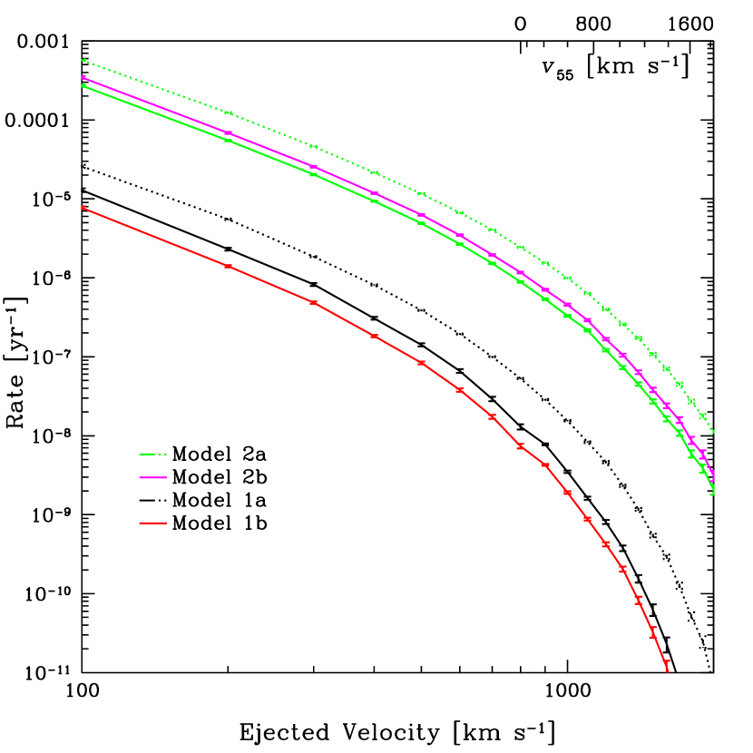
Figure 1: The total rate of stars with ejected velocities $v_{{\infty}}>v_{\rm ej}$ versus $v_{\rm ej}$ for $r_{\rm min}=0.001\,$pc. The coloured curves from top to bottom are for Models 2a (green), 2b (magenta), 1a (black) and 1b (red). The dashed curves are for the same stellar MFs but for a system of $15\,M_{\odot}$ BHs instead of $10\,M_{\odot}$. The top axis is labelled to show the corresponding velocity at a galactocentric radius of $55\,$kpc, $v_{\rm 55}$.

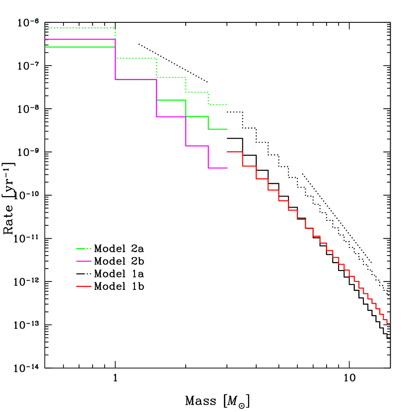
Figure 2: The total rate of HVSs ($v_{\rm ej}=1000\,{\rm km\,s}^{-1}$,) in $0.5\,M_{\odot}$ intervals for $r_{\rm min}=0.001\,$pc. The colours correspond to the same models as in Figure 1. The top and bottom black ‘dotted’ lines are for a power-law with slope -3, and -7 respectively for comparison. The discontinuity of the HVS rate at $3\,M_{\odot}$ is a result of our two different normalisations for Models 1 and 2.

The ejection rate also depends very strongly on the extent to which stars populate the innermost regions of the cusp, as shown in Figure 3. This is despite the constraints on the stellar DF (c.f. Eqs. 11 & 12), which limit both the semimajor axis of stars to $\sim\,0.01\,$pc and the maximum eccentricity of the orbit. For $r_{\rm min}\lesssim 0.001\,$pc the total rate increases with a shallow power-law index versus inner radius, doubling its value by $10^{-4}\,$pc. We caution, however, that interior to $0.001\,$pc, stellar collisions may flatten the cusp of low mass stars (Murphy et al., 1991; Freitag et al., 2006) and cause the rate of HVSs to increase more slowly than shown in Figure 3. For the high mass stars in the region (Models 1a-b), the stars are less likely to have physical collisions in their lifetimes, and may populate the entire phase space allowed by Eqs. (11) & (12).

Since Brown et al. (2006a) initiated a targeted search for HVSs in the Galactic halo, it is useful to forecast the number of observable HVSs that would originate from encounters with stellar-mass BHs. Current observations indicate that there are $\sim 33\pm 17$ hypervelocity B-stars with masses between $3$–$5\,M_{\odot}$ (W. Brown, private communication). Can scattered stars alone explain the abundance of the observed HVSs? The answer is positive but not under the most conservative conditions assumed thus far, which predict only $\sim 1(N_{\rm BH}/1800)$ such HVSs, for $r_{\rm min}=0.001\,$pc. If the masses of the BHs in the cluster were more typically $\sim 15\,M_{\odot}$, as might be expected from mass segregation as well as an old population of BHs (Belczynski et al., 2004), the number HVSs in our Galaxy would be four times larger. This is still lower than the number of observed HVSs. However, if we assume the most massive stars populate the entire phase space within the constraints of Eqs. (11) & (12), we expect there to be $\sim 30$ HVSs in our Galaxy. If we relax our definition of a HVS and set $v_{\rm ej}=900\,{\rm km\,s}^{-1}$, the ejection velocity of HVS7 (Carlberg & Innanen, 1987; Brown et al., 2006b), we get $\sim 50$ HVSs. The assumption that the stars fill the entire phase space is in best agreement with the observations of the S-stars, which appear to be a relaxed system (Ghez et al., 2005). By integrating the DF in this region, subject to the above constraints, we find that there should be $\lesssim 0.3$ stars interior to 0.001 pc. In addition, Equation (11) limits the semimajor axis of any star to $\sim 0.01$pc, close to the semimajor axis of S2 (S0-2), $\approx 0.005\,$pc. Thus, the stars that are ejected from this region are ones on eccentric orbits which bring them into this region, similar to S14 (S0-16), which has a closest approach of $\approx 0.0002\,$pc (Ghez et al., 2005). This is also consistent with the resonant relaxation timescales in the region (Rauch & Tremaine, 1996; Hopman & Alexander, 2006a, however, note our caution in § 5). We also note, however, that we are still being conservative in our calculations. We have excluded all collisional encounters, which at the highest relative velocities may not actually disrupt the star or have significant tidal energy dissipation. If stars and BHs do populate the inner $10^{-4}\,$pc, any collisions would be at velocities far greater than the escape velocity of the star. Our calculations suggest that such encounters may contribute a factor of a few more HVSs, and may offset any depletion of stars and BHs in the region. Since any such collisions would be brief and not very luminous (unless coalescence follows at low impact speeds), it would be difficult to identify star-BH collision events in external Galactic nuclei.

Most recently, Brown et al. (2007) have detected a significant number of marginally bound HVSs in the galactic halo. They found that these stars outnumber the unbound population by a factor of $\sim 2$. Such a ratio of bound to unbound HVSs is consistent with the scenario presented here, as well as the tidally ejected binary scenario Hills (1988) to within the statistical uncertainties (Brown et al., 2007). If we look at the ratio of the rates of stars ejected with velocities between $845\,{\rm km\,s}^{-1}$ ($v_{55}=275\,{\rm km\,s}^{-1}$) and $920\,{\rm km\,s}^{-1}$ ($v_{55}=450\,{\rm km\,s}^{-1}$), and stars ejected with higher velocities, we find that there should be $\approx 2.6$ times more bound HVSs than unbound HVSs in a volume limited survey. However, this analysis assumes that all such HVSs would be observable, and does not account for any selection effects of the survey by Brown et al. (2007). With more HVS discoveries, a more detailed statistical analysis may be able to determine the origin of the HVSs.

As we pointed out in § 3.3, the density profile of BHs assumed thus far will exceed the “drain limit” (Alexander & Livio, 2004) in the innermost regions of integration. We have therefore approximated the drain limit for both $10\,M_{\odot}$ and $15\,M_{\odot}$ BHs by using an $\alpha_{\rm BH}=1.7$ power-law, which we found to be the best fit to the Equation 1 of Alexander & Livio (2004) between $0.001$ and $0.1\,$pc. We assumed that, inside of $0.1\,$pc, there are $N_{\rm BH}\approx 12000$ $10\,M_{\odot}$ BHs and $\approx 5500$ $15\,M_{\odot}$ BHs. We have found that this increases the total rates calculated above by a factor of $\sim 4$ for the $10\,M_{\odot}$ BHs and $\sim 2$ for the $15\,M_{\odot}$ BHs. This is true, even if the BHs are drain limited only out to $\sim 0.01\,$pc. Thus, for a drain limited population of $10\,M_{\odot}$ BHs (interior to $0.01\,$pc), there would be $\sim 40$ hypervelocity B-stars produced from BH-star scattering, with $r_{\rm min}=0$.

Figure 3: The HVS ejection rate ($v_{\rm ej}=1000\,{\rm km\,s}^{-1}$) versus the minimum radius of integration $r_{\rm min}$. The lines are coloured as in Fig. 1. Interior to $0.001\,$pc, stellar collisions may flatten the cusp of low mass stars (Murphy et al., 1991; Freitag et al., 2006) and cause the rate of HVSs to increase more slowly than shown in Figure 3. For the high mass stars in the region (Models 1a-b), the stars are less likely to have physical collisions in their lifetimes, and may populate the entire phase space allowed by Eqs. (11) & (12).

5 Summary and discussion

We constructed a variety of models for the distribution of stars and BHs in the innermost $0.1\,$pc of the Galactic centre. Assuming that the cusp and disk of stars we observe today represent a steady state over the past $\sim\,100\,$Myr, we calculated the rate at which stars will scatter off BHs and populate the Milky Way halo. We showed that the total ejection rate of HVSs can be comparable to that produced by the tidal disruption of binaries, and may exceed it for intermediate mass stars. Our results are consistent with the total number of ejected stars from Fokker-Plank simulations by Freitag et al. (2006). Assuming that the B-stars are fully relaxed as is observed with the younger S-Stars (Ghez et al., 2005), we can account for most, if not all, of the stars observed by Brown et al. (2006a). We demonstrated that the velocity distribution as well as the mass distribution of HVSs should be truncated at high values for the BH scattering process compared to binary disruption events (see Figs. 1 and 2). Better statistics of HVS detections could therefore determine the relative significance of these two plausible channels.

In our study, the ejected stars originate from the inner $\sim 0.1\,$pc near Sgr A*, whereas the tidally disrupted binaries that produce HVSs originally come from $\gtrsim\,2\,$pc (Yu & Tremaine, 2003; Perets et al., 2006). The observations of the young disk of stars (Paumard et al., 2006), as well as the cluster of S-stars, suggest that the population of stars at 0.1 pc from Sgr A* should be younger and more massive than at $2\,$pc. This is further supported by the steep drop in B-stars outside of 0.5 pc (Paumard et al., 2006). In addition, binaries with B-stars ($t_{\rm ms}\lesssim 300\,$Myr) may also not be fully relaxed as has been assumed in many previous calculations, and therefore the diffusion rate of the most massive binaries into the loss-cone may be lower by orders of magnitudes.

In the survey of Brown et al. (2006b), the observed HVSs have the same colour as blue horizontal branch stars (BHBs) and have yet to be distinguished from B-stars with high resolution spectroscopy. The calculations shown here suggest that low mass stars, such as BHBs and their progenitors, can become HVSs with high efficiency if they are in the inner 0.1 pc of Sgr A*. Although tidal disruption rates may be enhanced by massive perturbers, BHBs must undergo significant mass loss, causing them to widen or even disrupt, and therefore are unlikely to be found in the tight binaries which are disrupted (Perets et al., 2006). The spectroscopic identification of one hypervelocity BHB star would be strong evidence in support of the mechanism presented here, or an inspiralling massive BH (Yu & Tremaine, 2003; Levin, 2005; Baumgardt et al., 2006). However, the expected rate of hypervelocity BHBs depends on uncertain details of stellar evolution and goes beyond the scope of this work. A population of BHBs ejected through this mechanism may be spun up through repeated encounters in the BH cusp (Alexander & Kumar, 2001), as well as during the final encounter which ejects them (H. Perets, private communication). Therefore, a rotating BHB star may appear to be more like a B-star without detailed spectroscopic evidence. In fact, the HVS HE 0437-5439 (Edelmann et al., 2005), should not be ruled out as being a BHB star based on its required spin value alone.

There is a curious link between the number of HVSs observed by Brown et al. (2006b) and the S-stars observed orbiting Sgr A*. Some S-stars may be the former companions to the HVSs from tidally disrupted binaries (Gould & Quillen, 2003; Ginsburg & Loeb, 2006; Perets et al., 2006). Interestingly, there exists a similar connection between HVSs scattered off of the BHs and the S-stars as well, although perhaps not one–to–one. For every strong encounter that produces a HVS, there is likely another encounter which can bring the star closer to Sgr A*, perhaps kicking out the BH instead, similar to the scenario proposed by Alexander & Livio (2004). In this scenario, the scattering of a small fraction of young stars from many previous disks into the inner $0.04\,$pc may result in a population similar to the S-stars (O’Leary, R. M. & Loeb, A. 2007, in preparation). However, we should note that if the S-star are in fact the remnants of tidally disrupted binaries, then this mechanism will only be secondary, as it is only ejects a small fraction of such stars.

There is obviously considerable uncertainty in our models. The rate of diffusion of stars both close to and far from Sgr A* into eccentric orbits is important to understanding both the mechanisms as well as the source of the observed B-type HVSs in the Galactic halo. In both cases, it is most likely that the stars formed on relatively circular orbits, whether in a disk around Sgr A* or in an inspiralling cluster. Large scale simulations similar to those already done by Freitag et al. (2006) can help resolve the uncertainties of relaxation, and with modifications, may be able to account for the conditions of continuous star formation over long periods of time. For low mass stars, physical collisions may deplete the total number of stars, and reduce the rate. In our discussion we have not considered the effects of resonant relaxation (Rauch & Tremaine, 1996; Hopman & Alexander, 2006a) near Sgr A*, which may have two counteracting effects on our rate calculation. Resonant relaxation may flatten the cusp and deplete the number density of stars and BHs in the innermost 0.01 pc; at the same time, it may also drive more massive stars into the same region producing more B-type HVSs (Hopman & Alexander, 2006a).

In our analysis, we also neglected the migration of massive objects near Sgr A*. If, as suggested by Portegies Zwart et al. (2006), many intermediate mass BHs (IMBHs with masses $\gtrsim 10^{3}\,M_{\odot}$) populate the inner pc of the Galactic centre and merge with Sgr A* every $\sim 10^{7}$–$10^{8}\,$yr, then the cusp of stellar-mass BHs and stars would not regenerate fast enough to produce HVSs through BH-star encounters (Baumgardt et al., 2006) but instead could produce them through IMBH-star encounters (Levin, 2005). BHs with masses between most stellar mass BHs and IMBHs (e.g. $\sim 50\,M_{\odot}$), may also form through standard binary evolution (Belczynski et al., 2004). Such BHs could considerably increase the rate of HVSs, even if they are relatively rare.

References

- Alexander (2005) Alexander T., 2005, Physics Reports, 419, 65
- Alexander & Kumar (2001) Alexander T., Kumar P., 2001, ApJ, 549, 948
- Alexander & Livio (2004) Alexander T., Livio M., 2004, ApJ, 606, L21
- Alexander & Sternberg (1999) Alexander T., Sternberg, A., 1999, ApJ, 520, 137
- Bahcall & Wolf (1976) Bahcall J. N., Wolf R. A., 1976, ApJ, 209, 214
- Bahcall & Wolf (1977) Bahcall J. N., Wolf R. A., 1977, ApJ, 216, 883
- Baumgardt et al. (2006) Baumgardt H., Gualandris A., Portegies Zwart S., 2006, MNRAS, 372, 174
- Belczynski et al. (2004) Belczynski, K., Sadowski, A., Rasio, F. A. 2004, ApJ, 611, 1068
- Binney & Tremaine (1987) Binney J., Tremaine S., 1987, Galactic dynamics. Princeton, NJ, Princeton University Press, 1987, 747 p.
- Bromley et al. (2006) Bromley B. C., Kenyon S. J., Geller M. J., Barcikowski E., Brown W. R., Kurtz M. J., 2006, ApJ, 653, 1194
- Brown et al. (2005) Brown W. R., Geller M. J., Kenyon S. J., Kurtz M. J., 2005, ApJ, 622, L33
- Brown et al. (2006a) Brown W. R., Geller M. J., Kenyon S. J., Kurtz M. J., 2006a, ApJ, 640, L35
- Brown et al. (2006b) Brown W. R., Geller M. J., Kenyon S. J., Kurtz M. J., 2006b, ApJ, 647, 303
- Brown et al. (2007) Brown, W. R., Geller, M. J., Kenyon, S. J., Kurtz, M. J., & Bromley, B. C. 2007, ArXiv Astrophysics e-prints, arXiv:astro-ph/0701600
- Carlberg & Innanen (1987) Carlberg R. G., Innanen K. A., 1987, AJ, 94, 666
- Deegan & Nayakshin (2007) Deegan P., Nayakshin S., 2007, MNRAS, 377, 897
- Edelmann et al. (2005) Edelmann H., Napiwotzki R., Heber U., Christlieb N., Reimers D., 2005, ApJ, 634, L181
- Eisenhauer et al. (2005) Eisenhauer F., Genzel R., Alexander T., Abuter R., Paumard T., Ott T., Gilbert A., Gillessen S., Horrobin M., Trippe S., Bonnet H., Dumas C., Hubin N., Kaufer A., Kissler-Patig M., Monnet G., Ströbele S., Szeifert T., Eckart A., Schödel R., Zucker S., 2005, ApJ, 628, 246
- Freitag et al. (2006) Freitag M., Amaro-Seoane P., Kalogera V., 2006, ApJ, 653, 1194
- Genzel et al. (2003) Genzel R., Schödel R., Ott T., Eisenhauer F., Hofmann R., Lehnert M., Eckart A., Alexander T., Sternberg A., Lenzen R., Clénet Y., Lacombe F., Rouan D., Renzini A., Tacconi-Garman L. E., 2003, ApJ, 594, 812
- Ghez et al. (2005) Ghez A. M., Salim S., Hornstein S. D., Tanner A., Lu J. R., Morris M., Becklin E. E., Duchêne G., 2005, ApJ, 620, 744
- Ginsburg & Loeb (2006) Ginsburg I., Loeb A., 2006, MNRAS, 368, 221
- Gnedin et al. (2005) Gnedin O. Y., Gould A., Miralda-Escudé J., Zentner A. R., 2005, ApJ, 634, 344
- Gould & Quillen (2003) Gould A., Quillen A. C., 2003, ApJ, 592, 935
- Gualandris et al. (2005) Gualandris A., Portegies Zwart S., Sipior M. S., 2005, MNRAS, 363, 223
- Hénon (1960) Hénon M., 1960, Annales d’Astrophysique, 23, 467
- Henon (1969) Henon M., 1969, A&A, 2, 151
- Hills (1988) Hills J. G., 1988, Nat, 331, 687
- Hills (1991) Hills J. G., 1991, AJ, 102, 704
- Hirsch et al. (2005) Hirsch H. A., Heber U., O’Toole S. J., Bresolin F., 2005, A&A, 444, L61
- Hopman & Alexander (2006a) Hopman C., Alexander T., 2006a, ApJ, 645, 1152
- Hopman & Alexander (2006b) Hopman C., Alexander T., 2006b, ApJ, 645, L133
- Levin (2005) Levin Y., 2006, ApJ, 653, 1203
- Miralda-Escudé & Gould (2000) Miralda-Escudé J., Gould A., 2000, ApJ, 545, 847
- Morris (1993) Morris M., 1993, ApJ, 408, 496
- Murphy et al. (1991) Murphy, B. W., Cohn, H. N., Durisen, R. H. 1991, ApJ, 370, 60
- Nayakshin et al. (2006) Nayakshin S., Dehnen W., Cuadra J., Genzel R., 2006, MNRAS, 366, 1410
- Nayakshin & Sunyaev (2005) Nayakshin S., Sunyaev R., 2005, MNRAS, 364, L23
- Paumard et al. (2006) Paumard T., Genzel R., Martins F., Nayakshin S., Beloborodov A. M., Levin Y., Trippe S., Eisenhauer F., Ott T., Gillessen S., Abuter R., Cuadra J., Alexander T., Sternberg A., 2006, ApJ, 643, 1011
- Perets et al. (2006) Perets H. B., Hopman C., Alexander T., 2007, ApJ, 656, 709
- Portegies Zwart et al. (2006) Portegies Zwart S. F., Baumgardt H., McMillan S. L. W., Makino J., Hut P., Ebisuzaki T., 2006, ApJ, 641, 319
- Rauch & Tremaine (1996) Rauch K. P., Tremaine S., 1996, New Astronomy, 1, 149
- Schaller et al. (1992) Schaller G., Schaerer D., Meynet G., Maeder A., 1992, A&AS, 96, 269
- Schödel et al. (2007) Schödel R., Eckart A., Alexander T., Merritt D., Genzel R., Sternberg A., Meyer L., Kul F., Moultaka J., Ott T., Straubmeier C., 2007, A&A, 469, 125
- Sesana et al. (2006) Sesana A., Haardt F., Madau P., 2006, ApJ, 651, 392
- Yu & Tremaine (2003) Yu Q., Tremaine S., 2003, ApJ, 599, 1129