Crossing the Phantom Divide

Abstract

We consider fluid perturbations close to the “phantom divide” characterised by $p=-\rho$ and discuss the conditions under which divergencies in the perturbations can be avoided. We find that the behaviour of the perturbations depends crucially on the prescription for the pressure perturbation $\delta p$. The pressure perturbation is usually defined using the dark energy rest-frame, but we show that this frame becomes unphysical at the divide. If the pressure perturbation is kept finite in any other frame, then the phantom divide can be crossed. Our findings are important for generalised fluid dark energy used in data analysis (since current cosmological data sets indicate that the dark energy is characterised by $p\approx-\rho$ so that $p<-\rho$ cannot be excluded) as well as for any models crossing the phantom divide, like some modified gravity, coupled dark energy and braneworld models. We also illustrate the results by an explicit calculation for the “Quintom” case with two scalar fields.

I Introduction

The discovery by the supernova surveys sn1 ; sn2 that the expansion of the universe is currently accelerating came as a great surprise to cosmologists. Within the standard cosmological framework of a nearly isotropic and homogeneous universe and an evolution described by General Relativity, this behaviour requires a component with a negative pressure $p<-\rho/3$, commonly dubbed dark energy. However, it is very difficult to understand why the dark energy should appear at such a low energy scale, and why it should start to dominate the overall energy density just now. Explaining its nature is correspondingly regarded as one of the most important problems in observational cosmology.

Current limits on the equation of state parameter $w=p/\rho$ of the dark energy seem to indicate that $p\approx-\rho$ cora ; wlim , sometimes even that $p<-\rho$ phantom , often called phantom energy caldwell . Although there is no problem to consider $w<-1$ for the background evolution, there are apparent divergencies appearing in the perturbations when a model tries to cross the “phantom divide” $w=-1$crossing . Even though this region may be unphysical at the quantum level cht ; Cline:2003gs , it is still important to be able to probe it, not least to test for alternative theories of gravity or higher dimensional models which can give rise to an effective phantom energy para ; nojiri ; vli ; vik2 ; kosh . It would certainly be unwise to build a strong bias like $w\geq-1$ into our analysis tools as long as experiments do not rule it out. In this paper we consider the evolution of the perturbations for models where $w$ crosses $-1$. We find that in many realistic cases the divergencies are only apparent and can be avoided. At the level of cosmological first order perturbation theory, there is no fundamental limitation that prevents an effective fluid from crossing the phantom divide.

The paper is organised as follows: We start with a short recapitulation of the first order perturbations in fluids, which also serves to define our notation. In section III we study the behaviour of barotropic fluids close to $p=-\rho$, concluding that this class of fluids cannot cross the phantom divide self-consistently. We allow for non-adiabatic perturbations in section IV and show that the phantom divide can now be crossed as long as we define the pressure perturbation in a frame that stays physical. We then illustrate the results with the Quintom model of two scalar fields before presenting our conclusions. The appendices finally discuss the calculation of the effective Quintom perturbations in more detail.

II First order perturbations

In this paper we use overdots to refer to derivatives with respect to conformal time $\eta$ which is related to the physical time $t$ by $dt=ad\eta$. We will denote the physical Hubble parameter with $H$ and with ${\mathcal{H}}$ the conformal Hubble parameter. For simplicity, we consider a flat universe containing only (cold dark) matter and a dark energy fluid, so that the Hubble parameter is given by

$$H^{2}=\left(\frac{1}{a}\frac{da}{dt}\right)^{2}=H_{0}^{2}\left[\Omega_{m}a^{-3}+\left(1-\Omega_{m}\right)f(a)\right]$$ (1)

where $f(a)=\exp\left[-3\int_{1}^{a}\frac{1+w(u)}{u}du\right]$, implying that the scale factor today is $a_{0}=1$. We will assume that the universe is filled with perfect fluids only, so that the energy momentum tensor of each component is given by

$$T^{\mu\nu}=\left(\rho+p\right)u^{\mu}u^{\nu}+p~{}g^{\mu\nu}.$$ (2)

where $\rho$ and $p$ are the density and the pressure of the fluid respectively and $u^{\mu}$ is the four-velocity. This is potentially a strong assumption for the dark energy, but a more general model should lead to more freedom in the dark energy evolution, not less.

We will consider linear perturbations about a spatially-flat background model, defined by the line of element:

$$ds^{2} = a^{2}\left[-\left(1+2A\right)d\eta^{2}+2B_{i}d{\eta}dx^{i}+\right.$$ (3)

$$\left.+\left(\left(1+2H_{L}\right)\delta_{ij}+2H_{Tij}\right)dx_{i}dx^{j}\right]$$

where $A$ is the scalar potential; $B_{i}$ a vector shift; $H_{L}$ is the scalar perturbation to the spatial curvature; $H_{T}^{ij}$ is the trace-free distortion to the spatial metric, see e.g. hu_lecture for more details.

The components of the perturbed energy moment tensor can be written as:

$$T_{0}^{0} = -\left(\bar{\rho}+\delta\rho\right)$$ (4)

$$T_{j}^{0} = \left(\bar{\rho}+\bar{p}\right)\left(v_{j}-B_{j}\right)$$ (5)

$$T_{0}^{i} = \left(\bar{\rho}+\bar{p}\right)v^{i}$$ (6)

$$T_{j}^{i} = \left(\bar{p}+\delta{p}\right)\delta_{j}^{i}+\bar{p}~{}\Pi_{j}^{i}.$$ (7)

Here $\bar{\rho}$ and $\bar{p}$ are the energy density and pressure of the homogeneous and isotropic background universe, $\delta\!\rho$ is the density perturbation, $\delta p$ is the pressure perturbation, $v^{i}$ is the vector velocity and $\Pi_{j}^{i}$ is the anisotropic stress perturbation tensor hu_lecture .

We want to investigate only the scalar modes of the perturbation equations. We choose the Newtonian gauge (also known as the longitudinal gauge) which is very simple for scalar perturbations because they are characterised by two scalar potentials $\psi$ and $\phi$; the metric Eq. (3) becomes:

$$ds^{2}=a^{2}\left[-\left(1+2\psi\right)d\eta^{2}+\left(1-2\phi\right)dx_{i}dx^{i}\right]$$ (8)

where we have set the shift vector $B_{i}=0$ and $H_{T}^{ij}=0$. The advantage of using the Newtonian gauge is that the metric tensor $g_{\mu\nu}$ is diagonal and this simplifies the calculations mabe .

The energy-momentum tensor components in the Newtonian gauge become:

$$T_{0}^{0} = -\left(\bar{\rho}+\delta\rho\right)$$ (9)

$$ik_{i}T_{0}^{i} = -ik_{i}T_{i}^{0}=\left(\bar{\rho}+\bar{p}\right)\theta$$ (10)

$$T_{j}^{i} = \left(\bar{p}+\delta p\right)\delta_{j}^{i}$$ (11)

where we have defined the variable $\theta=ik_{j}v^{j}$ which represents the divergence of the velocity field and we have also assumed that the anisotropic stress vanishes, $\Pi_{j}^{i}=0$ (implying $\phi=\psi$).

The perturbation equations are mabe :

$$\dot{\delta} = -\left(1+w\right)\left(\theta-3\dot{\psi}\right)-3\frac{\dot{a}}{a}\left(\frac{\delta p}{\bar{\rho}}-w\delta\right)$$ (12)

$$\dot{\theta} = -\frac{\dot{a}}{a}\left(1-3w\right)\theta-\frac{\dot{w}}{1+w}\theta+$$ (13)

$$+k^{2}\frac{\delta{p}/\bar{\rho}}{1+w}+k^{2}\psi.$$

As $w\rightarrow-1$ the terms containing $1/(1+w)$ will generally diverge. This can be avoided by replacing $\theta$ with a new variable $V$ defined via $V=\left(1+w\right)\theta$. This corresponds to rewriting the $0i$ component of the energy momentum tensor as $ik_{j}T_{0}^{j}=\bar{\rho}V$ which avoids problems if $T_{0}^{j}\neq 0$ when $\bar{p}=-\bar{\rho}$. Replacing the time derivatives by a derivative with respect to the scale factor $a$ (denoted by a prime), we obtain:

$$\delta^{\prime} = 3(1+w)\psi^{\prime}-\frac{V}{Ha^{2}}-3\frac{1}{a}\left(\frac{\delta p}{\bar{\rho}}-w\delta\right)$$ (14)

$$V^{\prime} = -(1-3w)\frac{V}{a}+\frac{k^{2}}{Ha^{2}}\frac{\delta p}{\bar{\rho}}+(1+w)\frac{k^{2}}{Ha^{2}}\psi.$$ (15)

In this form everything looks perfectly finite even at $w=-1$. But in order to close the system, we need to give an expression for the pressure perturbations. A priori this is a free choice which will describe some physical properties of the fluid. In the following we will consider several possible choices and discuss how they influence the behaviour of the fluid at the phantom divide. We will see how the specification of $\delta p$ determines if a fluid can cross the divide or not.

In addition to the fluid perturbation equations we need to add the equation for the gravitational potential $\psi$. If there are several fluids present, then the evolution of each of them will be governed by their own set of equations for their matter variables $\{\delta_{i},V_{i}\}$, linked by a common $\psi$ (which receives contributions from all the fluids). We use mabe ,

$$\psi^{\prime}=-\frac{1}{2a}\left(\frac{\sum_{i}\delta_{i}\bar{\rho}_{i}}{\sum_{i}\bar{\rho}_{i}}\right)-\left(\frac{k^{2}}{3H^{2}a^{2}}+1\right)\frac{\psi}{a}.$$ (16)

The evolution of a fluid is therefore governed by Eqs. (14) and (15), supplemented by a prescription for the internal physics (given by $\delta p$) and the external physics (through $\psi$ and $\psi^{\prime}$). There are two points worth emphasising. Firstly, the dark energy fluid perturbations cannot be self-consistently set to zero if $w\neq-1$. Even if $\delta=V=0$ on some initial hypersurface, it is unavoidable that perturbations will be generated by the presence of $\psi$. As this function describes physics external to the fluid, it cannot be controlled directly. Conceivably $\delta p$ could be chosen to cancel the external source of either $\delta$ or $V$, but not of both. Even then such a $\delta p$ would have to be incredibly fine-tuned as $\psi$ and $\psi^{\prime}$ depend on the evolution of the other fluids as well.

Secondly, we see that as $w\rightarrow-1$ the external sources are turned off. A fluid can therefore mimic a cosmological constant as then (and only then) $\delta=V=\delta p=0$ is a solution. This corresponds to an energy momentum tensor (2) with $T_{\mu\nu}=\bar{p}g_{\mu\nu}$, so that $\Lambda\sim\bar{\rho}$. However, in general the perturbations do not vanish even if $w=-1$. A perfect fluid is therefore in general not a cosmological constant even if $\bar{\rho}=-\bar{p}$.

To calculate perturbations in different gauges we need to introduce the coordinate transformation:

$$\eta = \tilde{\eta}+T$$ (17)

$$x^{i} = \tilde{x}^{i}+L^{i}.$$ (18)

the gauge transformation of the matter variables is then:

$$\tilde{\delta\rho} = \delta\rho+3\frac{\dot{a}}{a}\left(1+w\right)\bar{\rho}T$$ (19)

$$\frac{\tilde{\delta p}}{\bar{p}} = \frac{\delta p}{\bar{p}}+3\frac{\dot{a}}{a}\left(1+w\right)\frac{c_{a}^{2}}{w}T$$ (20)

$$\tilde{u} = u+\dot{L}$$ (21)

where we have introduced a new quantity $c_{a}^{2}=\dot{\bar{p}}/\dot{\bar{\rho}}$, called adiabatic sound speed.

III Barotropic fluids

We define a fluid to be barotropic if the pressure $p$ depends strictly only on the energy density $\rho$: $p=p(\rho)$. These fluids have only adiabatic perturbations, so that they are often called adiabatic. We can write their pressure as

$$p(\rho)=p(\bar{\rho}+\delta\rho)=p(\bar{\rho})+\left.\frac{dp}{d\rho}\right|_{\bar{\rho}}\delta\rho+O\left((\delta\rho)^{2}\right).$$ (22)

Here $p(\bar{\rho})=\bar{p}$ is the pressure of the isotropic and homogeneous part of the fluid. Introducing $N\equiv\ln a$ as a new time variable, we can rewrite the background energy conservation equation, $\dot{\bar{\rho}}=-3{\mathcal{H}}(\bar{\rho}+\bar{p})$ in terms of $w$,

$$\frac{dw}{dN}=\frac{d\bar{\rho}}{dN}\frac{dw}{d\bar{\rho}}=-3(1+w)\bar{\rho}\frac{dw}{d\bar{\rho}}.$$ (23)

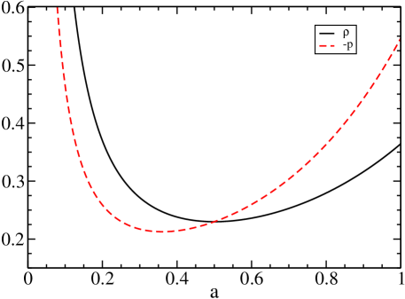
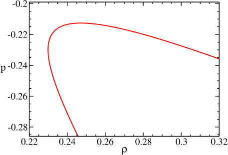
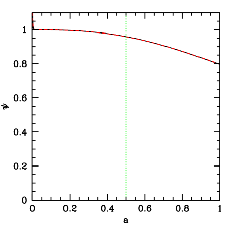
We see that the rate of change of $w$ slows down as $w\rightarrow-1$, and $w=-1$ is not reached in finite time vik1 , except if $dw/d\bar{\rho}$ diverges (or $\bar{\rho}$, but that would lead to a singular cosmology). The physical reason is that we demand $p$ to be a unique function of $\rho$, but at $w=-1$ we find that $\dot{\bar{\rho}}=0$. If the fluid crosses $w=-1$ the energy density $\rho$ will first decrease and then increase again, while the pressure $p$ will monotonically decrease (at least near the crossing), Fig. 1. It is therefore impossible to maintain a one-to-one relationship between $p$ and $\rho$, see Fig. 2 (notice that the maximum of $p$ and the minimum of $\rho$ do not coincide).

An example that can potentially cross $w=-1$ is given by

$$\left(1+w(\rho)\right)^{2}=C^{2}(\bar{\rho}-\bar{\rho}_{\times}).$$ (24)

Starting with $w>-1$ and $\bar{\rho}>\bar{\rho}_{\times}$ both will decrease until $w=-1$ and $\bar{\rho}=\bar{\rho}_{\times}$. If it is possible to switch from the branch with $w>-1$ to the other one at this point, then $\bar{\rho}$ can start to grow again while $w$ continues to decrease. Using the evolution equation (23) for $w$, we find

$$\frac{dw}{dN}=-\frac{3}{2}\left[C^{2}\bar{\rho}_{\times}+(1+w)^{2}\right]$$ (25)

so that $dw/dN\simeq-3/2C^{2}\bar{\rho}_{\times}$ near the crossing. The full solution (with $N=N_{\times}$ at $w=-1$) is

$$w(N)=-1-C\sqrt{\bar{\rho}_{\times}}\tan\left(\frac{3C\sqrt{\bar{\rho}_{\times}}}{2}(N-N_{\times})\right),$$ (26)

clearly not a realistic solution for our universe as there are divergencies in the finite past and future. Of course we could modify the example (24), but we are mostly interested at the behaviour near the crossing. In our case $1+w(a)\propto-(a-a_{\times})$, ie. we observe a linear behaviour. This is actually the limiting case: if we choose $(1+w)\propto(\bar{\rho}-\bar{\rho}_{\times})^{\nu}$ close to the crossing, we find

$$\frac{d(1+w)}{dN}\simeq-C(1+w)^{(2\nu-1)/\nu}$$ (27)

for small $|1+w|$. Correspondingly we cross with zero slope for $\nu>1/2$ and with infinite slope for $\nu<1/2$. However, if $dw/dN=0$ at $w=-1$ then the system will turn into a cosmological constant and stay there forever. On the other hand, this is unstable against small perturbations towards $\bar{p}<-\bar{\rho}$, so that the crossing might eventually be completed anyway.

Let us have a closer look at the perturbations. The second term in the expansion (22) can be re-written as

$$\left.\frac{dp}{d\rho}\right|_{\bar{\rho}}=\frac{\dot{\bar{p}}}{\dot{\bar{\rho}}}=w-\frac{\dot{w}}{3{\mathcal{H}}(1+w)}\equiv c_{a}^{2}$$ (28)

where we used the equation of state and the conservation equation for the dark energy density in the background. We notice that the adiabatic sound speed $c_{a}^{2}$ will necessarily diverge for any fluid where $w$ crosses $-1$.

Figure 1: Energy density (black solid line) and pressure (red dashed line) as functions of the scale factor. $w$ crosses $-1$ at $a_{\times}=0.5$, so that $\rho$ is minimal at this point while $p$ decreases monotonically there (but has a maximum earlier).

Figure 2: The pressure as function of the energy density. The graph of $p(\rho)$ shows that $p$ is not a single valued function of the energy density, and that there is a point with an infinite slope (corresponding to the minimum of $\rho$ and the divergence of ${c_{a}^{2}}$). The point where $p(\rho)$ has a zero slope corresponds to the maximum of $p$ and a vanishing ${c_{a}^{2}}$.

For a perfect barotropic fluid the adiabatic sound speed ${c_{a}^{2}}$ turns out to be the physical propagation speed of perturbations. It should therefore never be larger than the speed of light, otherwise our theory becomes acausal ah ; bcd . The condition ${c_{a}^{2}}\leq 1$ for $(1+w)>0$ (our point of departure) is equivalent to

$$-\frac{dw}{dN}\leq 3(1+w)(1-w).$$ (29)

No barotropic fluid can therefore pass through $w=\pm 1$ from above without violating causality. Even worse, the pressure perturbation

$$\delta p=c_{a}^{2}\delta\!\rho=\left(w-\frac{\dot{w}}{3{\mathcal{H}}(1+w)}\right)\delta\!\rho$$ (30)

will necessarily diverge if $w$ crosses $-1$ and $\delta\!\rho\neq 0$. Using the gauge transformation Eqs. (19) and (20) we see that the relation between pressure and energy density perturbations is gauge invariant. If the pressure perturbation diverges in one frame, it will diverge in all frames. The only possible way out would be to force $\delta\!\rho\rightarrow 0$ fast enough at the crossing. Let us study the behaviour close to $w=-1$ in some detail now:

First we look only at the dominant contribution to the right hand side of Eq. (14). Near $w=-1$ this is clearly:

$$\delta^{\prime}=-\frac{3}{a}{c_{a}^{2}}\delta=+\frac{w^{\prime}}{1+w}\delta.$$ (31)

Assuming that near the crossing the equation of state behaves like $1+w\approx\lambda(a-a_{\times})^{\alpha}$ with $\alpha>0$ we find the solution:

$$\delta\propto(a-a_{\times})^{\alpha}$$ (32)

(independent of $\lambda$ which drops out of the equation). This solution goes to zero at the crossing. If the sign had been different, we would have found instead the solution $\delta\propto(a-a_{\times})^{-\alpha}$ which diverges.

The pressure perturbation behaves like

$$\delta p\propto\bar{\rho}\left(\frac{\alpha a}{3}(a-a_{\times})^{\alpha-1}+{\cal O}((a-a_{\times})^{\alpha})\right).$$ (33)

We need $\alpha\geq 1$, otherwise the pressure perturbation will diverge as a power-law at the crossing. Unfortunately this condition is not sufficient. Looking at the second perturbation equation (15) we see that although nothing diverges, there is no reason for $V$ to go to zero at the crossing, and in general it will not, except if we fine-tune it with infinite precision. As $\delta$ vanishes at crossing and can so potentially cancel the divergence in the sound speed, this term is no longer necessarily dominant in the differential equation for $\delta$, Eq. (31). We also need to take into account the other contributions. The term containing $\psi^{\prime}$ is sufficiently suppressed by the $1+w$ factor to neglect it. Taking $V$ to be constant at $a_{\times}$ (to lowest order) $V(a_{\times})=V_{\times}$, we find:

$$\delta^{\prime}=-C_{\times}+\frac{w^{\prime}}{1+w}\delta$$ (34)

with $C_{\times}=V_{\times}/(H(a_{\times})a_{\times}^{2})$. The solution to this equation is:

$$\delta=\left\{\begin{array}[]{ll}(a-a_{\times})\left(\delta_{\times}-C_{\times}\log|a-a_{\times}|\right)&\alpha=1\\ \delta_{\times}(a-a_{\times})^{\alpha}+(a-a_{\times})C_{\times}/(1-\alpha)&\alpha\neq 1\end{array}\right.$$ (35)

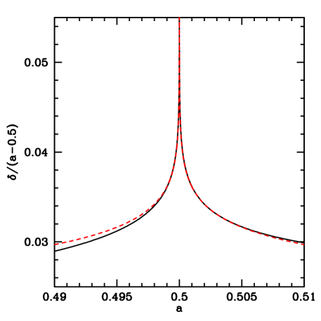
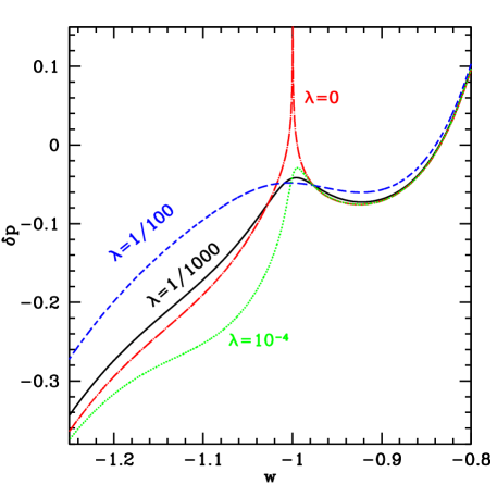
We notice that for $\alpha\geq 1$ the density perturbations vanish at crossing. However, for $\alpha=1$ they do not vanish fast enough. Instead of the behaviour given in Eq. (33), the pressure perturbation exhibits now a logarithmic divergence since the sound speed cancels the factor $(a-a_{\times})$. Even though our derivation here is not rigorous, numerical calculations confirm this behaviour, also if the background is not completely matter dominated, see Fig. 3. Although a full solution may be possible in some cases, it would turn out to be a special function, obscuring the structure of the result while still showing essentially the same simple behaviour.

Figure 3: This figure shows the logarithmic divergence of $\delta/(a-a_{\times})$ near $a_{\times}=0.5$. The black curve is the numerical solution while the red dashed line shows the approximation given by Eq. (35) for $\alpha=1$. The approximate formula describes the structure of the divergence quite well. The pressure perturbation $\delta p$ exhibits a very similar divergence in this case.

We find therefore three possible behaviours for the perturbations, depending on how $w$ crosses the phantom divide:

1. $\alpha<1$: In this case $w$ crosses $-1$ with an infinite slope, leading to a power-law divergence of the pressure perturbation.

2. $\alpha=1$: $w$ crosses $-1$ with a finite, but non-zero slope. $\delta\!\rho$ vanishes, $V$ stays finite and generally non-zero and $\delta p$ diverges logarithmically.

3. $\alpha>1$: $w$ crosses $-1$ with a zero slope. $\delta\!\rho$ vanishes, $V$ and $\delta p$ stay finite and generally non-zero.

The only acceptable case is the last one, but as discussed at the beginning of this section, we expect the system to get stuck at $w=-1$ and to never cross. Barotropic perfect fluids therefore fail to cross either at the background or perturbation level. Even if the fluctuations can lead to a crossing with zero slope due to the instability of the cosmological constant solution in some cases, the model is still not realistic. The perturbations seem to propagate acausally, and generically after the transition ${c_{a}^{2}}<0$ for a period, leading to classical instabilities with exponential growth of the perturbations. In the next section we will relax the barotropic assumption, which allows for entropy perturbations that can stabilise the system and keep the sound speed below the speed of light.

IV Non-adiabatic fluids

The discussion of the barotropic fluid shows that we have to violate the constraint that $p$ be a function of $\rho$ alone. At the level of first order perturbation theory, this amounts to changing the prescription for $\delta p$ which now becomes an arbitrary function of $k$ and $t$. This problem is conceptually similar to choosing the background pressure $\bar{p}(t)$, where the conventional solution is to compare the pressure with the energy density by setting $\bar{p}(t)=w(t)\bar{\rho}(t)$. In this way we avoid having to deal with a dimensionfull quantity and can instead set $w$, which has no units (up to a factor of the speed of light) and so is generically of order unity and often has a simple form, like $w=1/3$ for a radiation fluid or $w=-1$ for a cosmological constant.

It certainly makes sense to try a similar approach for the pressure perturbation. However, there are two relevant variables that we could compare $\delta p$ to, the fluid velocity $V$ and the perturbation in the energy density $\delta\!\rho$. Clearly it would be counterproductive to replace a single free function by two free functions, and it would lead to degeneracies between the two. Another problem is that the perturbation variables depend on the gauge choice. But in this case the two problems cancel each other, leading to a simpler solution: Going to the rest-frame of the fluid both fixes the gauge and renders the fluid velocity physically irrelevant, so that we can now write bedo :

$$\delta\hat{p}={\hat{c}_{s}^{2}}\delta\!\hat{\rho},$$ (36)

where a hat denotes quantities in the rest-frame. The physical interpretation is that ${\hat{c}_{s}^{2}}(k,t)$ is the speed with which fluctuations in the fluid propagate, ie. the sound speed. Again, some physical models lead to simple prescriptions for the sound speed. The barotropic models discussed in the last section have ${\hat{c}_{s}^{2}}(k,t)={c_{a}^{2}}(t)$, and the perturbations in a scalar field correspond (to linear order) exactly to those of a fluid with ${\hat{c}_{s}^{2}}(k,t)=1$.

The rest-frame is chosen so that the energy-momentum tensor looks diagonal to an observer in this frame. In terms of the gauge transformations this amounts to choosing $B=\theta_{\mathrm{DE}}$. However, we notice immediately a potential flaw in this prescription close to $w=-1$: The off-diagonal entries of the energy-momentum tensor are actually $(\bar{\rho}+\bar{p})\theta$ so that demanding $\theta-B=0$ is a stronger condition than required. In other words, the condition to be at rest with respect to the flow of $\bar{\rho}+\bar{p}$ cannot be maintained at $\bar{\rho}+\bar{p}=0$. However, as $\bar{\rho}>0$, we could define instead the sound speed in a frame where there is no flow of energy density.

To see this, let us calculate the pressure perturbation defined by Eq. (36) in the conformal Newtonian frame, following bedo : Breaking the single link between $\rho$ and $p$ amounts to the introduction of entropy perturbations. A gauge invariant entropy perturbation variable is $\Gamma\equiv\frac{\delta{p}}{\bar{p}}-\frac{c_{a}^{2}}{w}\frac{\delta\!\rho}{\bar{\rho}}$ KS ; bedo . By using

$$w\Gamma=\frac{\dot{p}}{\rho}\left(\frac{\delta p}{\dot{p}}-\frac{\delta\!\rho}{\dot{\rho}}\right)$$ (37)

and the expression for the gauge transformation of $\delta\!\rho$ KS ,

$$\delta\!\hat{\rho}=\delta\!\rho+3{\mathcal{H}}\bar{\rho}\frac{V}{k^{2}}$$ (38)

we find that the pressure perturbation is given by

$$\delta p={\hat{c}_{s}^{2}}\delta\!\rho+3{\mathcal{H}}\left({\hat{c}_{s}^{2}}-{c_{a}^{2}}\right)\bar{\rho}\frac{V}{k^{2}}.$$ (39)

As ${c_{a}^{2}}\rightarrow\infty$ at the crossing, it is impossible that all other variables stay finite except if $V\rightarrow 0$ fast enough. Again we will show that this is not in general the case, except if ${\hat{c}_{s}^{2}}\rightarrow 0$ or $w^{\prime}\rightarrow 0$ at crossing. However, we will then see that this is not required, indeed we will argue in the next section that the more generic solution is to let ${\hat{c}_{s}^{2}}$ diverge at the crossing in order to cancel the divergence of ${c_{a}^{2}}$!

To this end, we consider again the structure of the perturbation equations near $w=-1$. Inserting the expression for $\delta p$ into our system of perturbation equations we find

$$\delta^{\prime} = 3(1+w)\psi^{\prime}-\left(\frac{k^{2}}{Ha^{2}}+3H({\hat{c}_{s}^{2}}-{c_{a}^{2}})\right)\frac{V}{k^{2}}$$ (40)

$$-\frac{3}{a}\left({\hat{c}_{s}^{2}}-w\right)\delta$$

$$\frac{V^{\prime}}{k^{2}} = -\frac{1+3({c_{a}^{2}}-w-{\hat{c}_{s}^{2}})}{a}\frac{V}{k^{2}}+$$ (41)

$$+\frac{1+w}{Ha^{2}}\psi+\frac{{\hat{c}_{s}^{2}}}{Ha^{2}}\delta.$$

The spoiler here is the continued presence of ${c_{a}^{2}}$ which we know to diverge at crossing. Let us start by considering a finite and constant ${\hat{c}_{s}^{2}}$. For all reasonable choices of $k$ the dominant term in the $V$ equation will be the one containing ${c_{a}^{2}}$. We find that this time the velocity perturbation is driven to zero at crossing:

$$V^{\prime}=\frac{w^{\prime}}{1+w}V.$$ (42)

Proceeding as in the last section, we find that now $V\propto(a-a_{\times})^{\alpha}$, cancelling the divergence in ${c_{a}^{2}}$ for $\alpha\geq 1$. Now $\delta\!\rho$ will in general not vanish at crossing, and we have to include that term in the differential equation for $V$. The term with $\psi$ is suppressed by $1+w$ and is of higher order. As in the last section for $\delta$, the solutions for $V$ are now to lowest order:

$$V=\left\{\begin{array}[]{ll}(a-a_{\times})\left(V_{\times}-D_{\times}\log|a-a_{\times}|\right)&\alpha=1\\ V_{\times}(a-a_{\times})^{\alpha}+(a-a_{\times})D_{\times}/(1-\alpha)&\alpha\neq 1\end{array}\right.$$ (43)

with $D_{\times}$ being ${\hat{c}_{s}^{2}}k^{2}\delta/(Ha^{2})$, evaluated at crossing.

Again there are no divergences appearing in the energy momentum tensor only if $\alpha>1$, ie. if $w$ crosses $-1$ with a zero slope. A possible way to get around this fine-tuning is to demand that ${\hat{c}_{s}^{2}}=0$ at crossing, as in this case the logarithmically divergent term disappears. We also notice that the usual velocity perturbation $\theta\equiv V/(1+w)$ does diverge in all cases, either logarithmically if $\alpha=1$ or as $(a-a_{\times})^{1-\alpha}$ if $\alpha>1$. For an observer in the rest-frame where $B=\theta$ this means that the metric perturbations become large – at crossing the metric is even singular. At the very least, perturbation theory is no longer valid for such an observer.

Another way to see that the rest-frame is ill-defined is to look at the energy momentum tensor (2). For $p=-\rho$ the first term disappears, leaving us with $T^{\mu\nu}=p~{}g^{\mu\nu}$. Normally the four-velocity $u^{\mu}$ is the time-like eigenvector of the energy momentum tensor, but now suddenly all vectors are eigenvectors. The problem of fixing a unique rest-frame is therefore no longer well-posed.

However, by construction the pressure perturbation looks perfectly fine for precisely the observer in the rest-frame, as $\delta\hat{p}={\hat{c}_{s}^{2}}\delta\!\hat{\rho}$ does not diverge. Our prescription for the pressure perturbations has singled out the one frame which we cannot use for fluids crossing the phantom divide. The reason is that the gauge transformation relating the pressure perturbations in the different gauges is:

$$\delta\hat{p}=\delta p+3{\mathcal{H}}\bar{\rho}{c_{a}^{2}}\frac{V}{k^{2}}.$$ (44)

If $V$ does not vanish fast enough at the crossing then the pressure perturbation has to diverge in at least one frame. As we have just discussed, the dark-energy rest-frame becomes unphysical at crossing. It is clearly better to specify a finite pressure perturbation in a different frame.

One problem is to find a way of characterising the pressure perturbations in a physical way – in the Quintom example of the next section, we find that the additional contributions diverge but in such a way that we end up with a finite result for $\delta p$. As another example, we just choose $\delta p$ proportional to $\delta\!\rho$,

$$\delta p(k,t)=\gamma\,\delta\!\rho(k,t)$$ (45)

in the conformal Newtonian gauge. This will work as long as $\delta\!\rho\neq 0$, otherwise it forces $\delta p$ to vanish in the same place as $\delta\!\rho$, which is not general enough. If we insert this expression into eqs. (14) and (15), we obtain:

$$\delta^{\prime} = 3(1+w)\psi^{\prime}-\frac{V}{Ha^{2}}-3\frac{1}{a}\left(\gamma-w\right)\delta$$ (46)

$$V^{\prime} = -(1-3w)\frac{V}{a}+\frac{k^{2}}{Ha^{2}}\gamma\delta+(1+w)\frac{k^{2}}{Ha^{2}}\psi.$$ (47)

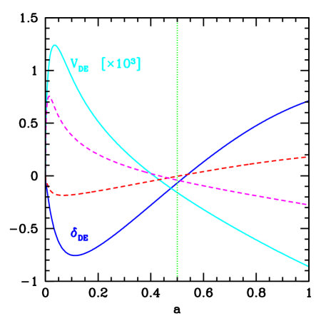
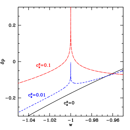
As $w\rightarrow-1$ none of the terms diverge, so that $\delta$ and $V$ stay in general finite and non-zero at crossing. We show in Figs. 4 and 5 a numerical example for two choices of $\gamma$ where it is impossible to see that the phantom divide has been crossed at $a_{\times}=0.5$.

Figure 4: This figure shows the density contrast $\delta_{\mathrm{DE}}$ (red and blue lines, negative for small scale factor $a$) and the velocity perturbation $V_{\mathrm{DE}}$ (cyan and magenta lines, positive for small $a$) for a dark energy component with a pressure perturbation given in the conformal Newtonian gauge through $\gamma$ (as defined in Eq. (45)). The solid lines show the results for $\gamma=0.2$ and the dashed lines for $\gamma=1$.The crossing of the phantom divide at $a_{\times}=0.5$ (dotted green vertical line) is not apparent in these figures, everything is finite.

Figure 5: The gravitational potential $\psi$ in the same scenario as Fig. 4 (with $\gamma=0.2$ for the black solid line and $\gamma=1$ for the red dashed line). Again, the crossing of the phantom divide at $a_{\times}=0.5$ (dotted green vertical line) is not apparent. The gravitational potential is constant during matter domination (small $a$) and starts to decay as the dark energy begins to dominate and the expansion rate of the universe accelerates. The contribution of the dark energy perturbations to $\psi$ is very small ($\,\raise 1.72218pt\hbox{$<$}\kern-8.00003pt\lower 2.6694pt\hbox{$\sim$}\,0.1\%$) so that there is no visible difference for the two choices of $\gamma$.

It is of course possible to express $\gamma$ in terms of ${\hat{c}_{s}^{2}}$, and ${\hat{c}_{s}^{2}}$ in terms of $\gamma$. Using the expression for the pressure perturbation in the rest-frame given by Eq. (36) and the gauge transformation given by Eqs. (19) and (20), we obtain

$$\gamma\delta\rho+3{\mathcal{H}}c_{a}^{2}\bar{\rho}\frac{V}{k^{2}}={\hat{c}_{s}^{2}}\left(\delta\!\rho+3{\mathcal{H}}\bar{\rho}\frac{V}{k^{2}}\right).$$ (48)

In general $\gamma$ will therefore be scale dependent even if ${\hat{c}_{s}^{2}}$ is not (even though of course ${\hat{c}_{s}^{2}}$ will also in general depend on $k$ and $t$), or vice versa. Also, to reproduce the evolution with finite $\gamma$ shown in Figs. 4 and 5 we would have to substitute a divergent ${\hat{c}_{s}^{2}}$ to cancel the divergence in ${c_{a}^{2}}$ (cf. figure 7 which shows how the apparent sound speed diverges in the Quintom example). We also notice that on very small scales where $k\gg 1$ we find $\gamma\approx{\hat{c}_{s}^{2}}$ for finite ${c_{a}^{2}}$, which is the usual result that on small scales gauge differences become irrelevant (for physical gauges).

Finally we would like to emphasise again that for a general, finite pressure perturbation in any gauge except the fluid rest-frame, there is no problem with the perturbation evolution across the phantom divide. Also, in general the perturbations, including $V$, will not vanish at crossing.

V The Quintom model as explicit example

To clarify some of the above points we consider an explicit example of a model crossing the phantom divide, the Quintom model quintom1 ; quintom2 , and compute the pressure perturbation ab initio at crossing (see also qpert ).

The original Quintom model considered two scalar fields. For us it is advantageous to use instead two fluids with a constant and equal rest-frame sound speed ${\hat{c}_{s}^{2}}=1$. At the level of first order perturbation theory the two models are exactly equivalent, see appendix A. As in the original model, we use two fluids with constant equations of state parameters $w_{1}$ and $w_{2}$. We will have to map the two fluids onto a single effective fluid. To this end we define the effective parameters in such a way that the effective energy momentum tensor is the sum of the two fluid energy momentum tensors. This leads to:

$$\bar{\rho}_{\mathrm{eff}} = \bar{\rho}_{1}+\bar{\rho}_{2}$$ (49)

$$\bar{p}_{\mathrm{eff}} = \bar{p}_{1}+\bar{p}_{2}$$ (50)

$$w_{\mathrm{eff}} = \frac{w_{1}\bar{\rho}_{1}+w_{2}\bar{\rho}_{2}}{\bar{\rho}_{1}+\bar{\rho}_{2}}$$ (51)

$$\delta_{\mathrm{eff}} = \frac{\bar{\rho}_{1}\delta_{1}+\bar{\rho}_{2}\delta_{2}}{\bar{\rho}_{1}+\bar{\rho}_{2}}$$ (52)

$$\theta_{\mathrm{eff}} = \frac{\left(1+w_{1}\right)\bar{\rho}_{1}\theta_{1}+\left(1+w_{2}\right)\bar{\rho}_{2}\theta_{2}}{\left(1+w_{1}\right)\bar{\rho}_{1}+\left(1+w_{2}\right)\bar{\rho}_{2}}.$$ (53)

Re-expressing the perturbation equations in these variables we find precisely the normal perturbation equations for a single fluid (14) and (15) with $\bar{p}_{\mathrm{eff}}$ and $\delta p_{\mathrm{eff}}$ replacing $p$ and $\delta p$. $\bar{p}_{\mathrm{eff}}$ is simply given by $w_{\mathrm{eff}}\bar{\rho}_{\mathrm{eff}}$, but the density perturbation is more involved. Starting from $\delta p_{\mathrm{eff}}=\delta p_{1}+\delta p_{2}$ we can write it as

$$\delta p_{\mathrm{eff}} = {\hat{c}_{s,\mathrm{eff}}^{2}}\delta\!\rho_{\mathrm{eff}}+\delta p_{{\mathrm{rel}}}+\delta p_{{\mathrm{nad}}}$$ (54)

$$+3{\mathcal{H}}\left({\hat{c}_{s,\mathrm{eff}}^{2}}-{c_{a}^{2}}\right)\bar{\rho}_{\mathrm{eff}}\frac{V_{\mathrm{eff}}}{k^{2}}$$

where the (effective) adiabatic sound speed is as always ${c_{a}^{2}}=\dot{\bar{p}}_{\mathrm{eff}}/\dot{\bar{\rho}}_{\mathrm{eff}}$ and where ${\hat{c}_{s,\mathrm{eff}}^{2}}=1$ for two scalar fields. The other terms are the relative pressure perturbation

$$\delta p_{{\mathrm{rel}}}=\frac{\left(w_{2}-w_{1}\right)\dot{\bar{\rho}}_{1}\dot{\bar{\rho}}_{2}}{3{\mathcal{H}}\dot{\bar{\rho}}_{\mathrm{eff}}}S_{12}$$ (55)

given by the relative density perturbation of the two scalar fields,

$$S_{12}=\frac{\delta_{1}}{1+w_{1}}-\frac{\delta_{2}}{1+w_{2}}$$ (56)

(which corresponds to a gauge invariant relative entropy perturbationMaWa ) as well as the non-adiabatic term

$$\delta p_{{\mathrm{nad}}}=-\left(w_{2}-w_{1}\right)\frac{\dot{\bar{\rho}}_{1}\dot{\bar{\rho}}_{2}}{3{\mathcal{H}}\dot{\bar{\rho}}_{\mathrm{eff}}}\left[S_{12}+\frac{3{\mathcal{H}}}{k^{2}}\Delta\theta_{12}\right]$$ (57)

given by the relative motion of the two scalar fields with $\Delta\theta_{12}=\theta_{1}-\theta_{2}$ (see appendix C).

We notice that the relative perturbations act as internal perturbations which couple to the effective variables purely through the behaviour of the pressure perturbation. Understanding the physics behind the dark energy in such a case will therefore require a precise measurement of the pressure perturbations as well as their careful analysis, to uncover the different internal contributions.

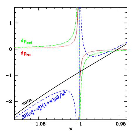
Even though the effective sound speed ${\hat{c}_{s,\mathrm{eff}}^{2}}=1$ in Eq. (54) is finite in the rest-frame, the transformation to any other frame will lead to a divergence as discussed in the previous section. This divergence then needs to be cancelled by the two additional terms, $\delta p_{{\mathrm{rel}}}$ and $\delta p_{{\mathrm{nad}}}$. In our example, both diverge, cancelling together the divergent contribution from the singular gauge transformation as well as their own divergencies, see Fig. 6. This behaviour, which looks extremely fine-tuned, is automatically enforced in this model. Such a cancellation mechanism is required for any model in order to cross $w=-1$.

Figure 6: This figure shows the different divergent contributions to the pressure perturbation, Eq. (54), multiplied by $10^{9}$. The relative pressure perturbation is shown as red dotted line, the non-adiabatic pressure perturbation as green dash-dotted line and the contribution from the gauge transformation to the conformal Newtonian frame as blue dashed line. Each of the contributions diverges at the phantom crossing, but their sum (shown as black solid line), and so $\delta p$, stays finite.

We also see that although the effective sound speed remains simply ${\hat{c}_{s}^{2}}=1$, this is only true if we know that there are internal relative and non-adiabatic pressure perturbations (as well as their form). But in general we would try to parametrise the pressure perturbation as:

$$\delta p_{\mathrm{eff}}=c_{x}^{2}\delta\!\rho_{\mathrm{eff}}+3{\mathcal{H}}\left(c_{x}^{2}-{c_{a}^{2}}\right)\bar{\rho}_{\mathrm{eff}}\frac{V_{\mathrm{eff}}}{k^{2}}.$$ (58)

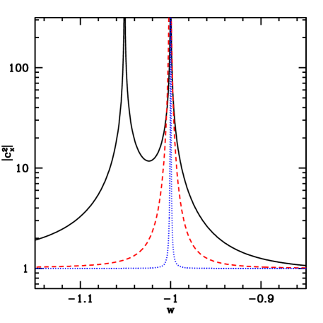
where the apparent sound speed $c_{x}^{2}$ is now a mixture of the real effective sound speed together with the relative and the non-adiabatic pressure perturbations. In this case we no longer find a simple form for the sound speed. In Fig. 7 we plot $c_{x}^{2}$ as a function of the equation of state parameter $w$ for several wave vectors $k$. As predicted, the apparent rest-frame sound speed diverges at the crossing. In the Quintom case the effective perturbations do not vanish at $w=-1$.

Figure 7: We plot the apparent sound speed $c_{x}^{2}$ defined by Eq. (58) for three different wave vectors, $k=1/H_{0}$ (black solid line), $k=10/H_{0}$ (red dashed line) and $100/H_{0}$ (blue dotted line). Although the real sound speed is just ${\hat{c}_{s}^{2}}=1$, the apparent sound speed diverges at $w=-1$ and can even become negative.

We think that the lessons learned from the Quintom model are applicable also to more general models with multiple fields, non-minimally coupled scalar fields, brane-world models and other modified gravity models that can be represented by an effective dark energy fluid. In all these models, as in the Quintom case, $w_{\mathrm{eff}}=-1$ is not a special point in their evolution. There is no reason to expect that the model will adjust its behaviour at this point, as the crossing of the phantom divide is incidential. In representing these kinds of models with an effective fluid we therefore expect that the perturbations will not vanish, and that the apparent sound speed would have to diverge.

One important difference between the Quintom model and more general modified gravity models is that the latter seem to require generically a non-zero anisotropic stress as $\phi\neq\psi$ ks_mg . In this case ${\hat{c}_{s}^{2}}=0$ does not allow crossing the phantom divide, since $D_{\times}$ in Eq. (43) contains an additional non-zero term due to the anisotropic stress. This reinforces our view that the Quintom-like crossing, where all perturbations stay non-zero and $\delta p_{\mathrm{eff}}$ remains finite in spite of divergences in most conventionally expected terms, is more generic. This means that there is no obvious way to predict the form of $\delta p_{\mathrm{eff}}$ in general for modified gravity models. On the positive side, if the dark energy is not just a cosmological constant, and if we are able to measure $\delta p_{\mathrm{eff}}$ then we may hope that this will provide us with clues about the physical mechanism that is causing the accelerated expansion of the universe.

VI Conclusions

As long as the cosmological data indicates the presence of a dark energy with an effective equation of state $p\approx-\rho$ it will be necessary to consider models with the same equation of state. In general, we will have to allow the equation of state to cross the phantom divide, $w=-1$. Even though such a fluid model may not be viable at the quantum level, it is possible that this behaviour is only apparent, or due to a modification of General Relativity or the existence of more spatial dimensions. In analysing the data we therefore have to be able to use general self-consistent models at the level of linear perturbation theory.

In this paper we have studied the behaviour of the perturbations in general perfect fluid models close to $w=-1$. We have shown that although models with purely adiabatic perturbations cannot cross $w=-1$ without violating important physical constraints (like causality or smallness of the perturbations), it is possible to rectify the situation by allowing for non-adiabatic sources of pressure perturbations. However, the parametrisation of $\delta p$ in terms of the rest-frame perturbations of the energy density cannot be used as this frame becomes unphysical at $w=-1$. By parameterising $\delta p$ instead in any other frame the divergencies are avoided.

We also computed all quantities in the Quintom model which provides an explicit example of the above mechanism. In this model, even though the propagation speed of sound waves remains finite and constant, the additional internal and relative pressure perturbations lead to an apparent sound speed which diverges. It is only the sum of all contributions to $\delta p$ which remains finite.

A more speculative conclusion is that it seems difficult for “fundamental” fields to cross $w=-1$ as their apparent rest-frame sound speed, defined through Eq. (36), would generally be the actual propagation speed of their perturbations, which must remain smaller than the speed of light. From the discussion in section IV we learn that fields with a well defined rest-frame and sound speed have only two routes to phantom crossing:

• $dw/da=0$ at crossing: This looks rather fine-tuned as the field needs to be aware of the presence of the barrier. On the other hand, a normal minimally coupled scalar field reaches $w=-1$ when $\dot{\phi}=0$, and it does so with zero slope. A scenario where phantom crossing of this kind is realised could be built by changing the sign in front of the kinetic term whenever $\dot{\phi}=0$. As an example, a cosine potential then leads to a “phaxion” scenario, see Fig. 8. On average, the phaxion behaves like a cosmological constant, but oscillates around $w=-1$. However, it is unclear how to construct such a scenario in a covariant way.

• vanishing sound speed: A field with a vanishing sound speed can also avoid the logarithmic divergence of $\delta p$. This requires either a coupling between $1+w$ and ${\hat{c}_{s}^{2}}$ or else the sound speed might be zero at all times, see Fig. 9. In the latter case the pressure of the field would need to remain close to $-\rho$ at all times in order to prevent the small-scale perturbations from growing too quickly. Also, the sound speeds needs to be exactly zero, otherwise the logarithmic divergence reappears. This may require a symmetry enforcing ${\hat{c}_{s}^{2}}=0$ as even a very small but non-zero sound speed would render this scenario inviable.

In view of these difficulties, the Quintom family of models, although more complicated than a single field, may prove to be the conceptually simplest way to cross $w=-1$ with a model defined through an action. They also illustrate that the effective pressure perturbation may provide a kind of fingerprint of the mechanism behind the accelerated expansion of the universe if it can be measured.

Figure 8: The phaxion: The sign in front of the kinetic term of a normal scalar field is flipped every time $\dot{\phi}$ passes through zero (so that $\dot{\phi}\geq 0$). As potential we use $V(\phi)=1+\cos(\phi/m_{0})$ which is bounded both from above and below. The field then moves to large values (top left graph), while $w$ oscillates around $-1$ (top right). The energy density $\rho$ also oscillates so that the field mimics an effective cosmological constant (bottom left). As the phantom divide is crossed with zero slope, there is no divergence in the pressure perturbation (bottom right), but the time-dependent effective mass can lead to strong growth of the perturbations in spite of ${\hat{c}_{s}^{2}}=1$.

Figure 9: The pressure perturbation $\delta p$ for three fluids with different rest-frame sound speed, ${\hat{c}_{s}^{2}}=0.1$ (top curve, red dash-dotted line), ${\hat{c}_{s}^{2}}=0.01$ (middle curve, blue dashed line) and ${\hat{c}_{s}^{2}}=0$ (lowest, solid line). Only the last case does not have a logarithmic divergence in the pressure perturbation at the phantom divide.

Concerning the use of phantom-crossing fluids for the purpose of data analysis, it is straightforward to implement them by just avoiding the usual parametrisation of the pressure perturbations in terms of the rest-frame sound speed. However, there does not seem to be a canonical way to choose the pressure perturbations if one is not allowed to use the dark energy rest-frame. The aim for the far future will be to directly measure the pressure perturbations of the dark energy in order to gain insight into the physical origin of the phenomenon. For now, we have to ensure that the definition of $\delta p$ does not lead to unphysical situations, while preserving the usual parametrisation in terms of the rest-frame sound speed as much as possible far away from the phantom divide. Maybe the simplest way out is to regularise the adiabatic sound speed ${c_{a}^{2}}$ which appears in Eq. (39) because of the gauge transformation into the rest-frame. While any finite choice of $\delta p$ is a physically acceptable choice, it is preferable to modify Eq. (39) in a minimal way so that the usual interpretation of ${\hat{c}_{s}^{2}}$ is preserved for $w\neq-1$. We propose to use

$$\tilde{c}_{a}^{2}=w-\frac{\dot{w}(1+w)}{3{\mathcal{H}}[(1+w)^{2}+\lambda]}$$ (59)

where $\lambda$ is a tuneable parameter which determines how close to $w=-1$ the regularisation kicks in. A value of $\lambda\approx 1/1000$ should work reasonably well, as shown in Fig. 10. In this case $\delta p$ is well-defined and there are no divergencies appearing in the perturbation equations (40) and (41). Although the differences in $\delta p$ for the different choices of $\lambda$ in Fig. 10 look important, we have to remember that, firstly, the perturbations in the dark energy are normally small (especially close to the phantom divide) and that secondly they are only communicated to the other fluids via the gravitational potential $\psi$. As in Fig. 5, we find also here that the dark energy perturbations are subdominant. Computing the CMB power spectrum for $\lambda=1/100$ and $\lambda=10^{-4}$ we find a relative difference in the $C_{\ell}$ of less than 1% on large scales, which rapidly drops to $10^{-6}$ by $\ell=50$, well below cosmic variance. We expect detectable differences only for strongly clustering dark energy with a sound speed that is close to zero or even negative. Although it is reassuring that directly measureable quantities are not sensitive to the precise value of $\lambda$ in Eq. (59), this also shows that it will be very difficult to distinguish between different models of dark energy if $w\approx-1$.

Figure 10: The pressure perturbation for a fluid example with ${\hat{c}_{s}^{2}}=0.1$. The red dash-dotted curve shows the standard case with the logarithmic divergence at $w=-1$. The blue (dashed), black (solid) and green (dotted) curve use a regularised adiabatic sound speed $\tilde{c}_{a}^{2}$ which does not diverge. The black curve with $\lambda=1/1000$ provides a reasonable fit. Larger values smooth too much, while smaller values start to follow the divergence and exhibit a temporary instability in the solution for $V$.

Appendix A Equivalence between scalar fields and fluid models

The aim of this appendix is to show that at the level of first-order perturbation theory a scalar field behaves just like a non-adiabatic fluid with ${\hat{c}_{s}^{2}}=1$. To this end we decompose the scalar field into a homogeneous mode $\phi(t)$ and a perturbation $\delta\phi(k,t)$. At the background level we find

$$\bar{\rho} = \frac{1}{2a^{2}}\dot{\phi}^{2}+V\left(\phi\right)$$ (60)

$$\bar{p} = \frac{1}{2a^{2}}\dot{\phi}^{2}-V\left(\phi\right)$$ (61)

and the equation of conservation is just the equation of motion,

$$\ddot{\phi}+2{\mathcal{H}}\dot{\phi}+a^{2}\frac{dV}{d\phi}=0.$$ (62)

The adiabatic sound speed is defined as:

$${c_{a}^{2}}=\frac{\dot{\bar{p}}}{\dot{\bar{\rho}}}=\frac{-\frac{3aH}{a^{2}}\dot{\phi}^{2}-2\frac{dV}{d\phi}\dot{\phi}}{-\frac{3aH}{a^{2}}\dot{\phi}^{2}}=1+\frac{2a}{3H}\frac{\frac{dV}{d\phi}}{\dot{\phi}}$$ (63)

(and we remind the reader that $\dot{a}/a={\mathcal{H}}=aH$). The perturbed energy momentum tensor is:

$$-\delta T_{0}^{0} = \delta\rho=\frac{1}{a^{2}}\dot{\phi}\dot{\delta\phi}-\frac{1}{a^{2}}\dot{\phi}^{2}\Psi+\frac{dV}{d\phi}\delta\phi$$ (64)

$$\delta T_{i}^{i} = \delta p=\frac{1}{a^{2}}\dot{\phi}\dot{\delta\phi}-\frac{1}{a^{2}}\dot{\phi}^{2}\Psi-\frac{dV}{d\phi}\delta\phi$$ (65)

$$-ik\delta T_{0}^{i} = ik\delta T_{i}^{0}=\frac{k^{2}}{a^{2}}\dot{\phi}\delta\phi=\bar{\rho}V$$ (66)

where we wrote $\Psi$ for the gravitational potential $\psi$ in order to avoid confusions with the scalar field variables (only in this appendix).

In order to derive the rest frame sound speed ${\hat{c}_{s}^{2}}$ of the scalar field we use equation (39)

$$\delta p={\hat{c}_{s}^{2}}\delta\rho+\frac{3aH}{k^{2}}\left({\hat{c}_{s}^{2}}-{c_{a}^{2}}\right)\bar{\rho}V$$ (67)

and express everything in terms of scalar field quantities. We find

$$\frac{1}{a^{2}}\dot{\phi}\dot{\delta\phi}-\frac{1}{a^{2}}\dot{\phi}^{2}\Psi-\frac{dV}{d\phi}\delta\phi=$$

$$={\hat{c}_{s}^{2}}\left(\frac{1}{a^{2}}\dot{\phi}\dot{\delta\phi}-\frac{1}{a^{2}}\dot{\phi}^{2}\Psi+\frac{dV}{d\phi}\delta\phi+\frac{3aH}{a^{2}}\dot{\phi}\delta\phi\right)-$$

$$-\frac{3aH}{a^{2}}\left(1+\frac{2a}{3H}\frac{1}{\dot{\phi}}\frac{dV}{d\phi}\right)\dot{\phi}\delta\phi$$ (68)

which after some algebraic manipulations turns into

$$\frac{1}{a^{2}}\dot{\phi}\dot{\delta\phi}-\frac{1}{a^{2}}\dot{\phi}^{2}\Psi+\frac{dV}{d\phi}\delta\phi+\frac{3aH}{a^{2}}\dot{\phi}\delta\phi=$$

$$={\hat{c}_{s}^{2}}\left(\frac{1}{a^{2}}\dot{\phi}\dot{\delta\phi}-\frac{1}{a^{2}}\dot{\phi}^{2}\Psi+\frac{dV}{d\phi}\delta\phi+\frac{3aH}{a^{2}}\dot{\phi}\delta\phi\right).$$ (69)

Therefore ${\hat{c}_{s}^{2}}=1$.

Now let us derive the equation of motion for the scalar field perturbations from the perturbation equation for a perfect fluid, Eq. (12),

$$\dot{\delta}=-\left(1+w\right)\left(\theta-3\dot{\Psi}\right)-3aH\left(\frac{\delta p}{\bar{\rho}}-w\delta\right)$$ (70)

which can be rewritten as

$$\dot{\delta\rho}+3aH\left(\bar{\rho}+\bar{p}\right)\delta=3\left(\bar{\rho}+\bar{p}\right)\dot{\Psi}-\rho V$$ (71)

Expressing the time derivative $\delta\rho$ in terms of scalar field quantities,

$$\dot{\delta\rho} = -\frac{2aH}{a^{2}}\dot{\phi}\dot{\delta\phi}+\frac{1}{a^{2}}\ddot{\delta\phi}\dot{\phi}-\frac{2aH}{a^{2}}\dot{\phi}\dot{\delta\phi}-\frac{dV}{d\phi}\dot{\delta\phi}-$$

$$-\frac{1}{a^{2}}\dot{\phi}^{2}\dot{\Psi}+\frac{6aH}{a^{2}}\dot{\phi}^{2}\Psi+2\dot{\phi}\frac{dV}{d\phi}\Psi+\frac{dV}{d\phi}\dot{\delta\phi}+\frac{d^{2}V}{d\phi^{2}}\dot{\phi}\delta\phi$$

and doing likewise with the other terms,

$$3aH\left(\delta\rho+\delta p\right) = \frac{6aH}{a^{2}}\dot{\phi}\dot{\delta\phi}-\frac{6aH}{a^{2}}\dot{\phi}^{2}\Psi$$ (73)

$$3\left(\bar{\rho}+\bar{p}\right)\dot{\Psi} = \frac{3}{a^{3}}\dot{\phi}^{2}\dot{\Psi}$$ (74)

$$\bar{\rho}V = \frac{k^{2}}{a^{2}}\dot{\phi}\delta\phi$$ (75)

we can insert all these expressions into Eq. (71) and obtain finally

$$\ddot{\delta\phi}+2aH\dot{\delta\phi}+a^{2}\left(\frac{d^{2}V}{d\phi^{2}}+\frac{k^{2}}{a^{2}}\right)\delta\phi=4\dot{\phi}\dot{\Psi}-2a^{2}\Psi\frac{dV}{d\phi}$$ (76)

which is indeed the equation of motion for $\delta\phi$ in the conformal Newtonian gauge (see e.g. hu_lecture ).

Appendix B Effective perturbations in two barotropic fluids

We consider first two barotropic perfect fluids with constant equation of state parameters,

$$\bar{p}_{1}=w_{1}\bar{\rho}_{1},\quad w_{1}>-1;$$ (77)

$$\bar{p}_{2}=w_{2}\bar{\rho}_{2},\quad w_{2}<-1.$$ (78)

We can define the effective quantities as those appearing in the sum of the two energy-momentum tensors,

$$\bar{\rho}_{\mathrm{eff}} = \bar{\rho}_{1}+\bar{\rho}_{2}$$ (79)

$$\bar{p}_{\mathrm{eff}} = \bar{p}_{1}+\bar{p}_{2}$$ (80)

$$w_{\mathrm{eff}} = \frac{w_{1}\bar{\rho}_{1}+w_{2}\rho_{2}}{\bar{\rho}_{1}+\bar{\rho}_{2}}$$ (81)

$$\delta_{\mathrm{eff}} = \frac{\bar{\rho}_{1}\delta_{1}+\bar{\rho}_{2}\delta_{2}}{\bar{\rho}_{1}+\bar{\rho}_{2}}$$ (82)

$$\theta_{\mathrm{eff}} = \frac{\left(1+w_{1}\right)\bar{\rho}_{1}\theta_{1}+\left(1+w_{2}\right)\bar{\rho}_{2}\theta_{2}}{\left(1+w_{1}\right)\bar{\rho}_{1}+\left(1+w_{2}\right)\bar{\rho}_{2}}.$$ (83)

The system above is characterized by four variables $\delta_{1}$, $\delta_{2}$, $\theta_{1}$, $\theta_{2}$. In order to have a complete mapping, we need to introduce two more variables which express two internal degrees of freedom MaWa :

$$S_{12} = \frac{\delta_{1}}{1+w_{1}}-\frac{\delta_{2}}{1+w_{2}}$$ (84)

$$\Delta\theta_{12} = \theta_{1}-\theta_{2}$$ (85)

called respectively, relative entropy perturbation and the relative velocity of the two fluids.

We can now calculate the perturbation equation for the effective fluid from

$$T^{\mu}_{{}_{(eff)}\nu;\mu}=T^{\mu}_{{}_{(1)}\nu;\mu}+T^{\mu}_{{}_{(2)}\nu;\mu}=0$$ (86)

The $T^{\mu}_{0;\mu}$ and $T^{\mu}_{\nu;\mu}$ components give the perturbation equations:

$$\bar{\rho}_{1}\dot{\delta}_{1}+\bar{\rho}_{2}\dot{\delta}_{2}-3\dot{\phi}\left[\left(1+w_{1}\right)\bar{\rho}_{1}+\left(1+w_{2}\right)\bar{\rho}_{2}\right]+$$

$$+\left[\left(1+w_{1}\right)\bar{\rho}_{1}\theta_{1}+\left(1+w_{2}\right)\bar{\rho}_{2}\theta_{2}\right]+$$

$$+3{\mathcal{H}}\left[\delta p_{1}-w_{1}\bar{\rho}_{1}\delta_{1}+\delta p_{2}-w_{2}\bar{\rho}_{2}\delta_{2}\right]=0$$ (87)

the derivative of $\dot{\delta}_{\mathrm{eff}}$ is:

$$\dot{\delta}_{\mathrm{eff}} = \frac{\bar{\rho}_{1}\dot{\delta}_{1}+\bar{\rho}_{2}\dot{\delta}_{2}}{\bar{\rho}_{1}+\bar{\rho}_{2}}-3{\mathcal{H}}\frac{w_{1}\bar{\rho}_{1}\delta_{1}+w_{2}\bar{\rho}_{2}\delta_{2}}{\bar{\rho}_{1}+\bar{\rho}_{2}}+$$ (88)

$$+3{\mathcal{H}}\frac{w_{1}\bar{\rho}_{1}+w_{2}\bar{\rho}_{2}}{\bar{\rho}_{1}+\bar{\rho}_{2}}\frac{\bar{\rho}_{1}\delta_{1}+\bar{\rho}_{2}\delta_{2}}{\bar{\rho}_{1}+\bar{\rho}_{2}}$$

inserting the last one into Eq. (87) and remembering Eqs. (79) to (84), we have:

$$\dot{\delta}_{\mathrm{eff}} = -\left(1+w_{\mathrm{eff}}\right)\left(\theta_{{\mathrm{eff}}}-3\dot{\psi}\right)$$ (89)

$$-3{\mathcal{H}}\left(\frac{\delta p_{\mathrm{eff}}}{\bar{\rho}_{\mathrm{eff}}}-w_{\mathrm{eff}}\delta_{\mathrm{eff}}\right)$$

where $\delta p_{\mathrm{eff}}=\delta p_{1}+\delta p_{2}$. This is just the equation (12) for the effective quantities.

For the second perturbation equation we have:

$$\left(1+w_{1}\right)\bar{\rho}_{1}\dot{\theta}_{1}+\left(1+w_{2}\right)\bar{\rho}_{2}\dot{\theta}_{2}+$$

$$+4{\mathcal{H}}\left[\left(1+w_{1}\right)\bar{\rho}_{1}\theta_{1}+\left(1+w_{2}\right)\bar{\rho}_{2}\theta_{2}\right]+$$

$$-3{\mathcal{H}}\left[\left(1+w_{1}\right)^{2}\bar{\rho}_{1}\theta_{1}+\left(1+w_{2}\right)^{2}\bar{\rho}_{2}\theta_{2}\right]+$$

$$-k^{2}\psi\left[\left(1+w_{1}\right)\bar{\rho}_{1}+\left(1+w_{1}\right)\bar{\rho}_{1}\right]+$$

$$-k^{2}\left(\delta p_{1}+\delta p_{2}\right)=0$$ (90)

the derivative of $\theta_{\mathrm{eff}}$ is:

$$\dot{\theta}_{\mathrm{eff}} = \frac{\left(1+w_{1}\right)\bar{\rho}_{1}\dot{\theta}_{1}+\left(1+w_{2}\right)\bar{\rho}_{2}\dot{\theta}_{2}}{\left(1+w_{1}\right)\bar{\rho}_{1}+\left(1+w_{1}\right)\bar{\rho}_{1}}+$$ (91)

$$-3{\mathcal{H}}\frac{\left(1+w_{1}\right)^{2}\bar{\rho}_{1}\theta_{1}+\left(1+w_{2}\right)^{2}\bar{\rho}_{2}\theta_{2}}{\left(1+w_{1}\right)\bar{\rho}_{1}+\left(1+w_{1}\right)\bar{\rho}_{1}}+$$

$$+3{\mathcal{H}}\frac{\left(1+w_{1}\right)\bar{\rho}_{1}\theta_{1}+\left(1+w_{2}\right)\bar{\rho}_{2}\theta_{2}}{\left(1+w_{1}\right)\bar{\rho}_{1}+\left(1+w_{1}\right)\bar{\rho}_{1}}\times$$

$$\times\frac{\left(1+w_{1}\right)^{2}\bar{\rho}_{1}+\left(1+w_{2}\right)^{2}\bar{\rho}_{2}}{\left(1+w_{1}\right)\bar{\rho}_{1}+\left(1+w_{1}\right)\bar{\rho}_{1}}$$

again inserting the last one into Eq. (90) and remembering Eqs. (79) to(83) and (84), we obtain the expression for the second perturbation equation:

$$\dot{\theta}_{\mathrm{eff}} = -{\mathcal{H}}\left(1-3w_{\mathrm{eff}}\right)-\frac{\dot{w}_{\mathrm{eff}}}{1+w_{\mathrm{eff}}}\theta_{\mathrm{eff}}$$ (92)

$$+k^{2}\left[\frac{\delta p_{\mathrm{eff}}/\bar{\rho}_{\mathrm{eff}}}{1+w_{\mathrm{eff}}}+\psi\right]=0$$

Again, this is the same equation as the one for a single perfect fluid, Eq. (13). The difference to the general case is that now the pressure perturbations are fixed by the barotropic nature of the two fluids. Starting from the generic expression

$$\delta p_{\mathrm{eff}}=\delta p_{1}+\delta p_{2}=w_{1}\bar{\rho}_{1}\delta_{1}+w_{2}\bar{\rho}_{2}\delta_{2}$$ (93)

we find that the effective pressure perturbation is

$$\delta p_{\mathrm{eff}}={c_{a}^{2}}\delta_{\mathrm{eff}}-\frac{1}{3{\mathcal{H}}}\frac{\left(w_{2}-w_{1}\right)\dot{\bar{\rho}}_{1}\dot{\bar{\rho}}_{2}}{\dot{\bar{\rho}}_{\mathrm{eff}}}S_{12}$$ (94)

where ${c_{a}^{2}}$ is the adiabatic sound speed and is given by

$${c_{a}^{2}} = \frac{\dot{\bar{p}}_{\mathrm{eff}}}{\dot{\bar{\rho}}_{\mathrm{eff}}}=\frac{w_{1}\dot{\bar{\rho}}_{1}+w_{2}\dot{\bar{\rho}}_{2}}{\dot{\bar{\rho}}_{1}+\dot{\bar{\rho}}_{2}}=$$ (95)

$$= \frac{w_{1}\left(1+w_{1}\right)\bar{\rho}_{1}+w_{2}\left(1+w_{2}\right)\bar{\rho}_{2}}{\left(1+w_{1}\right)\bar{\rho}_{1}+\left(1+w_{2}\right)\bar{\rho}_{2}}.$$

The second term appearing in Eq. (94) can be considered as the relative pressure perturbation due to the relative motion:

$$\delta p_{{\mathrm{rel}}}=-\frac{\left(w_{2}-w_{1}\right)\dot{\bar{\rho}}_{1}\dot{\bar{\rho}}_{2}}{3{\mathcal{H}}\dot{\bar{\rho}}_{\mathrm{eff}}}S_{12}$$ (96)

A single barotropic fluid has the pressure perturbation $\delta p={c_{a}^{2}}\delta\!\rho$. For the two-fluid case we find an additional part coming from the relative perturbations of the two fluids. The new variable $S_{12}$ given by Eq. (84) is a gauge invariant relative entropy perturbation MaWa .

The time evolution of $S_{12}$ is given simply by:

$$\dot{S}_{12}=-\Delta\theta_{12},$$ (97)

and contains the fourth variable $\Delta\theta_{12}$, which is a relative velocity perturbation and evolves according to

$$\partial_{t}\Delta\theta_{12} = -{\mathcal{H}}\Delta\theta_{12}+3{\mathcal{H}}\left(w_{1}+w_{2}-c^{2}_{a}\right)\Delta\theta_{12}+$$ (98)

$$+k^{2}\left(w_{1}+w_{2}-c^{2}_{a}\right)S_{12}+$$

$$+3{\mathcal{H}}\left(w_{1}-w_{2}\right)\theta_{\mathrm{eff}}+k^{2}\frac{w_{1}-w_{2}}{1+w_{\mathrm{eff}}}$$

Appendix C Effective perturbations in the Quintom model

Perturbations in barotropic fluids with constant $w<0$ grow very rapidly due to the imaginary sound speed, ${c_{a}^{2}}=w<0$. A realistic model crossing the phantom divide needs therefore to be composed of fluids with non-adiabatic fluctuations and a positive sound speed. In the case of the Quintom model, we are dealing with two fluids with ${\hat{c}_{s}^{2}}=1$. As in appendix B, we define the effective quantities via eq. (79) - eq. (85): using these equations we find the relations between the variables of the two fluids and the variables of the effective fluid:

$$\delta_{1} = \frac{1+w_{1}}{1+w_{\mathrm{eff}}}\delta_{\mathrm{eff}}-$$ (99)

$$-\frac{\left(1+w_{1}\right)\left(1+w_{2}\right)\left(w_{\mathrm{eff}}-w_{1}\right)}{\left(1+w_{\mathrm{eff}}\right)\left(w_{2}-w_{1}\right)}S_{12}$$

$$\delta_{2} = \frac{1+w_{2}}{1+w_{\mathrm{eff}}}\delta_{\mathrm{eff}}-$$ (100)

$$-\frac{\left(1+w_{1}\right)\left(1+w_{2}\right)\left(w_{2}-w_{\mathrm{eff}}\right)}{\left(1+w_{\mathrm{eff}}\right)\left(w_{2}-w_{1}\right)}S_{12}$$

$$\theta_{1} = \theta_{\mathrm{eff}}+\frac{\left(1+w_{2}\right)\left(w_{\mathrm{eff}}-w_{1}\right)}{\left(1+w_{\mathrm{eff}}\right)\left(w_{2}-w_{1}\right)}\Delta\theta_{12}$$ (101)

$$\theta_{2} = \theta_{\mathrm{eff}}+\frac{\left(1+w_{1}\right)\left(w_{\mathrm{eff}}-w_{2}\right)}{\left(1+w_{\mathrm{eff}}\right)\left(w_{2}-w_{1}\right)}\Delta\theta_{12}$$ (102)

What we need to evaluate again in the Quintom model is the effective pressure perturbation, because all the other terms are the same. Taking the sum of the pressure perturbation defined in the rest-frame, we have:

$$\delta p_{\mathrm{eff}} = {\hat{c}_{s,1}^{2}}\delta\!\rho_{1}+{\hat{c}_{s,2}^{2}}\delta\!\rho_{2}+$$ (103)

$$+3{\mathcal{H}}\left(1+w_{1}\right)\left({\hat{c}_{s,1}^{2}}-w_{1}\right)\bar{\rho}_{1}\frac{\theta_{1}}{k^{2}}+$$

$$+3{\mathcal{H}}\left(1+w_{2}\right)\left({\hat{c}_{s,2}^{2}}-w_{2}\right)\bar{\rho}_{2}\frac{\theta_{2}}{k^{2}}$$

inserting the Eqs. (99) - (102) in Eq. (103) we find:

$$\delta p_{\mathrm{eff}}={\hat{c}_{s,\mathrm{eff}}^{2}}\delta\!\rho_{\mathrm{eff}}+\delta p_{{\mathrm{rel}}}+\delta p_{{\mathrm{nad}}}$$

$$+3{\mathcal{H}}\left({\hat{c}_{s,\mathrm{eff}}^{2}}-{c_{a}^{2}}\right)\left(1+w_{\mathrm{eff}}\right)\bar{\rho}_{\mathrm{eff}}\frac{\theta_{\mathrm{eff}}}{k^{2}}$$ (104)

where ${\hat{c}_{s,\mathrm{eff}}^{2}}$ is the effective rest-frame sound speed; $\delta p_{{\mathrm{rel}}}$ is the relative pressure perturbation and $\delta p_{{\mathrm{nad}}}$ is the non adiabatic contribution to the pressure perturbation; they are:

$${\hat{c}_{s,\mathrm{eff}}^{2}} = \frac{{\hat{c}_{s,1}^{2}}\left(1+w_{1}\right)\bar{\rho}_{1}+{\hat{c}_{s,2}^{2}}\left(1+w_{2}\right)\bar{\rho}_{2}}{\left(1+w_{1}\right)\bar{\rho}_{1}+\left(1+w_{2}\right)\bar{\rho}_{2}}$$ (105)

$$\delta p_{{\mathrm{rel}}} = \frac{\left(w_{2}-w_{1}\right)\dot{\bar{\rho}}_{1}\dot{\bar{\rho}}_{2}}{3{\mathcal{H}}\dot{\bar{\rho}}_{\mathrm{eff}}}S_{12}$$ (106)

$$\delta p_{{\mathrm{nad}}} = -\left[\left({\hat{c}_{s,1}^{2}}-{\hat{c}_{s,2}^{2}}\right)+\left(w_{2}-w_{1}\right)\right]\frac{\dot{\bar{\rho}}_{1}\dot{\bar{\rho}}_{2}}{3{\mathcal{H}}\dot{\bar{\rho}}_{\mathrm{eff}}}\times$$ (107)

$$\times\left[S_{12}+\frac{3{\mathcal{H}}}{k^{2}}\Delta\theta_{12}\right]$$

The total number of degrees of freedom remains the same when we change from the “two fluid” to the “single effective fluid” picture. In both cases we have four variables. What changes is the way these variables interact. In the two fluid case, the interaction proceeds through the gravitational potential $\psi$. In the single effective fluid picture, the additional degrees of freedom become internal and appear through additional contributions to the pressure perturbation $\delta p$.

References

- (1) A. G. Riess et al., Astronomical J. 116, 1009 (1998).
- (2) S. Perlmutter et al., Astrophys. J. 517, 565 (1999).
- (3) P.S. Corasaniti et al., Phys. Rev. D 70 083006 (2004).
- (4) D.N. Spergel et al., astro-ph/0603449 (2006).
- (5) U. Alam et al., Mon. Not. Roy. Astron. Soc. 354 275 (2004).
- (6) R.R. Caldwell, Phys. Lett. B 545, 23 (2002).
- (7) R.R. Caldwell and M. Doran, Phys. Rev. D 72, 043527 (2005).
- (8) S.M. Carroll, M. Hoffmann and M. Trodden, Phys. Rev. D 68, 023509 (2003).
- (9) J. M. Cline, S. Jeon and G. D. Moore, Phys. Rev. D 70, 043543 (2004).
- (10) L. Perivolaropoulos, JCAP 0510, 001 (2005).
- (11) S. Nojiri and S.D. Odintsov, Gen. Rel. Grav. 38, 1285 (2006).
- (12) M. Li, B. Feng and X. Zhang, JCAP 0512, 002 (2005).
- (13) A. Anisimov, E. Babichev and A. Vikman, JCAP 0506, 006 (2005).
- (14) I.Ya. Aref’eva, A.S. Koshelev and S.Yu. Vernov, Phys. Rev. D 72, 064017 (2005).
- (15) W. Hu, lecture notes, astro-ph/0402060 (2004).
- (16) C.P. Ma and E. Bertschinger, Astrophys. J. 455, 7 (1995).
- (17) A. Vikman, Phys. Rev. D 71, 023515 (2005).
- (18) A. Adams et al., hep-th/0602178 (2006).
- (19) C. Bonvin, C. Caprini, R. Durrer, astro-ph/0606584 (2006).
- (20) R. Bean and O. Doré, Phys. Rev. D 69, 083503 (2004).
- (21) H. Kodama and M. Sasaki, Progr. Theor. Phys. Suppl. 78, 1 (1984).
- (22) B. Feng, X. Wang and X. Zhang, Phys. Lett. B 607, 35 (2005).
- (23) W. Hu, Phys. Rev. D 71, 047301 (2005).
- (24) G.-B. Zhao et al., Phys. Rev. D 72, 123515 (2005).
- (25) K. A. Malik and D. Wands, JCAP 0502, 007 (2005).
- (26) M. Kunz and D. Sapone, astro-ph/0612452 (2006).
- (27) Sean M. Carroll, An Introduction to General Relativity SpaceTime and Geometry (Addison Wesley, 2004)
- (28) R. Durrer. Gauge Invariant Cosmological perturbation Theory, Fund. Cosmic Phys. 15, 209 (1994).