An improved deprojection and PSF-deconvolution technique for galaxy-cluster X-ray surface-brightness profiles

We have developed a regularisation procedure for the direct deprojection and PSF-deconvolution of X-ray surface brightness profiles of clusters of galaxies. This procedure allows us to obtain accurate density profiles in a straightforward manner from X-ray observations (in particular data from XMM-Newton, where the PSF correction is important), while retaining information about substructure in the gas distribution, in contrast to analytic modelling of the profiles. In addition to describing our procedure, we present here a detailed investigation of the accuracy of the method and its error calculations over a wide range of input profile characteristics and data quality using Monte Carlo simulations. We also make comparisons with gas density profiles obtained from Chandra observations, where the PSF correction is small, and with profiles obtained using analytic modelling, which demonstrate that our procedure is a useful improvement over standard techniques. This type of method will be especially valuable in the ongoing analysis of unbiased and complete samples of X-ray clusters, both local and distant, helping to improve the quality of their results.

1 Introduction

The density distribution of X-ray-emitting gas in galaxy clusters is an important probe of the underlying mass distribution. By assuming hydrostatic equilibrium and spherical symmetry, the total mass distribution can be obtained from the gas density profile $\rho_{\rm gas}(r)$ and temperature profile $T(r)$. The use of galaxy clusters to test structure formation models and as cosmological probes is reliant on these techniques. However, observations also suggest that non-gravitational processes can have important effects on the gas properties of galaxy clusters (e.g. Arnaud, 2005 for a review), which raises questions about our understanding of the links between gas and dark matter properties of clusters. Key diagnostics are provided by the gas entropy distribution, $S=T/\rho_{\rm gas}^{2/3}$, which reflect the specific thermo-dynamical history of the gas. (e.g. Ponman, Cannon & Navarro 1999; Ponman, Sanderson & Finoguenov 2003; Voit 2005; Pratt, Arnaud & Pointecouteau 2006). It is therefore essential to be able to accurately measure the gas distributions of clusters, not only so as to be able to make accurate inferences about their dark matter properties, but also to investigate the departures of the gas properties from the self-similar models expected in the absence of effects such as cooling and non-gravitational heating and feedback.

Surface brightness profiles of the X-ray emission from galaxy clusters have been the primary tool for studying their gas distributions since cluster data became available from early X-ray missions. Until recently, it was thought that (with the exception of central cooling flows) cluster profiles could be adequately fitted with a standard analytical $\beta$ model profile in surface brightness (e.g. Neumann & Arnaud 1999). However, the substantial increase in the data quality of cluster observations in the era of Chandra and XMM-Newton has revealed that cluster gas distributions are considerably more complex than expected, e.g. from ROSAT data. A variety of increasingly complicated analytical models have been used to fit cluster surface brightness profiles (e.g. Pratt & Arnaud 2002; Vikhlinin et al. 2006) and to calculate the corresponding gas density profile; however, the need for such a range of models, which are not generally physically motivated, is unsatisfactory. In addition, using an analytical model means that full information about real structure in the cluster profile is lost in converting the profile from surface brightness to emission measure.

One alternative is direct deprojection of measured surface brightness profiles (e.g. Fabian et al. 1981; Kriss et al. 1983; White et al. 1997). If we consider a spherical distribution of cluster gas, with a density distribution (or emission measure distribution, $S_{emit}(r)$) consisting of a series of concentric spherical shells of radii $r_{0},r_{1},..,r_{i},..,r_{n}$, then using simple geometric considerations (e.g. McLaughlin 1999) we can calculate a 2-D matrix $[R_{proj}]$ whose elements consist of the contributions of each shell $i$ to the projected emission measure in a series of annuli on the plane of the sky $j$ having radii $R_{0},R_{1},..,R_{i},..,R_{n}$ (which may be the same or different to the $r_{i}$), e.g. element $R_{proj,ij}$ is the fraction of the emission from shell $i$ that is observed in annulus $j$. For the purposes of this work, we consider a square matrix $R_{proj}$, with $R_{0}=r_{0}$, $R_{1}=r_{1}$, etc, so that the matrix has dimensions $n\times n$, where $n$ is the number of bins in the observed surface brightness profile. The product $[R_{proj}][S_{emit}]$ is then the 2-D emission measure profile as would be observed by a perfect detector. We can then calculate a second redistribution matrix, $[R_{PSF}]$ that takes into account the effect of the instrumental PSF, i.e. $R_{psf,jk}$ is the fraction of counts from annulus $j$ of the ‘ideal’ profile that are redistributed by the telescope into annulus $k$ in the final observed surface brightness profile (we assume that the energy dependence of the PSF is negligible). The relationship between an observed $S_{X}$ profile, $C_{obs}(R)$ and the originating 3D emission profile, $S_{emit}(r)$ can therefore be expressed as follows:

$$[C_{obs}]=[R_{PSF}][R_{proj}][S_{emit}]$$ (1)

where $C_{obs}(i)$ is the surface brightness detected in an annulus $i$, $S_{emit}(j)$ is the emission measure produced by a 3-D shell $j$, $R_{proj}(i,j)$ represents the fraction of emission from shell $j$ that would be observed by a perfect detector to fall in annulus $k$, and $R_{PSF}(i,k)$ a second redistribution of counts from an annulus $k$ of the ideal profile to annulus $i$ of the actual profile resulting from the effect of the PSF. $R_{proj}$ depends only on the geometry of the cluster (see e.g. McLaughlin 1999) and can be easily calculated, and $R_{PSF}$ can also be calculated based on knowledge of the optical properties of a given instrument.

However, it is not straightforward to solve Equation 1 directly, as it is an inverse problem: small amounts of noise in the data become greatly amplified in the solution for $S_{emit}$. This has limited the usefulness of such an approach for the analysis of cluster profiles, particularly for an instrument such as XMM-Newton with a reasonably large PSF. The use of “onion-skin” deprojection techniques is common for spectral analysis, and has also been applied to surface brightness profiles from Chandra (e.g. David et al. 2001); however, the “onion-skin” approach is heavily dependent on the choice of outermost bin. For Equation 1 to be accurate, it is necessary to take account of the contribution to each annulus from shells outside the outermost annulus chosen for the analysis (we discuss this further in Section 2). Finally, it is necessary to convert the resulting emission measure profiles to gas density profiles taking into account the variation of the cooling function $\Lambda(T,Z)$ with radius.

This paper describes the application of a regularisation technique to the direct deprojection and PSF-deconvolution of X-ray surface brightness profiles that has allowed us to overcome these limitations. Our method is motivated by, and adapted from, work by Bouchet (1995) on the deconvolution of gamma-ray spectra. In the following section, we describe the regularisation procedure in more detail. We then present in Section 3 the results of a range of tests using simulated data that demonstrate the reliability of our technique and its applicability to a wide range in data quality and cluster properties. In Section 4, we apply our technique to real data from XMM-Newton and Chandra and demonstrate that it performs well in comparison to other methods. Finally, in Section 5, we investigate the effect of using gas density profiles obtained from our method on the calculation of the logarithmic slope and thus total mass profiles for clusters.

2 Method for regularised deprojection and PSF-deconvolution

Our method for regularising the deprojection/PSF-deconvolution process is motivated by the analysis of Bouchet (1995) on the deconvolution of gamma-ray spectra. The general method is to introduce additional constraints on the solution of Equation 1 based on prior information, in this case simply the expectation that the solution should be smooth, rather than unphysically noisy (see Sections 2.1 and 2.2). It is then necessary to introduce a means of balancing the regularisation constraint with the accuracy to which the solution reproduces the data (parameterised by $\chi^{2}$). As described by Bouchet, this is done by using Lagrangian multipliers to find a solution, then minimising the function

$$L(f,\lambda)=\chi^{2}(f)+\lambda C(f)$$ (2)

where $f$ is the solution, $C(f)$ a function that is a minimum when the solution best satisfies the regularity constraint, and $\lambda$ is the smoothing parameter. By varying $\lambda$, we can therefore vary the degree to which the solution is dominated by consistency with the data or with the regularising constraints. The choice of $\lambda$ is therefore critical to obtaining a reliable solution, and is described further in Section 2.2.

2.1 The regularisation constraint

Again following Bouchet (1995), we adopt the Philips-Towmey regularisation method (Phillips 1962; Towmey 1963). Generally, this method consists of minimizing the sum of the squares of the $k^{th}$ order derivates of the solution around each datapoint. For our purposes, we define the “smoothness” constraint as the minimum in the deviation of the solution from a constant about each data point, so that:

$$C(f)=\sum_{j=2}^{N-1}(f_{j-1}+f_{j})^{2}$$ (3)

Since our data covers several orders of magnitude in surface brightness, it is necessary to reduce the dynamic range of the problem by rescaling the data by a rough best-fitting model. Bouchet found that the choice of scaling function only affected the solution for low signal-to-noise data or when the model fit to the data was poor. We initially used a $\beta$ model to scale the data, and found that in cases where the fit was poor (caused by the data being more centrally peaked than can be represented by a $\beta$ model) the solution tended to bias towards a flatter profile; however, this affected only the central few bins. We then adopted the AB model of Pratt & Arnaud (2002), which is a modified version of the $\beta$ model that can roughly fit both centrally peaked and cored models. This model was tested on a large sample of clusters and found to achieve adequate fits in all cases with no systematic residuals at the centre. It is therefore better suited as a scaling function for our regularisation procedure, and we demonstrate in Section 3 that our rescaling procedure using the AB model does not lead to any bias in the output emission measure and gas density profiles. The regularisation constraint is therefore applied to the rescaled data.

Figure 1: Results of Monte Carlo simulations of the deprojection and PSF deconvolution of surface brigthness profiles corresponding to different shapes of the input model density profiles, as indicated in the individual plot labels. The simulated surface brightness profiles have a global S/N ratio of 200, for a total source/background count ratio of $R=0.3$. In all cases, the mean output density profile and errors are shown by red squares, with the input density model profile indicated by a black solid line.

Figure 2: Same simulations as for Fig. 1. The mean output profile of $d\log{n_{e}}/d\log{r}$ and errors are shown by red squares, with the profile obtained from the input density model indicated by a black solid line.

Figure 3: Monte Carlo simulations of the deprojection and PSF deconvolution of “bumpy” surface brightness profiles. The lefthand density profile is a beta model with sinusoidal variations superimposed, and the righthand profile is a beta model with a density jump, such as might be produced by a cold front. Red symbols are the output profile; solid black line is the input model.

Figure 4: Results of Monte Carlo simulations of the deprojection and PSF deconvolution of surface brigthness profiles with different global S/N ratios and source/background count ratios $R$ ($3\sigma$ binning in cases), as indicated in the individual plot labels. In all cases, the mean output density profile and errors are shown by red squares, with the input density model profile indicated by a black solid line.

Figure 5: Same simulations as Fig. 4. The mean output profile of $d\log{n_{e}}/d\log{r}$ and errors are shown by red squares, with the profile obtained from the input density model indicated by a black solid line.

Figure 6: Results of Monte Carlo simulations of the deprojection and PSF deconvolution of surface brigthness profiles, using different binning of the data (signal-to-noise per bin), as indicated in the individual plot labels. The simulated surface brigthness profiles have a global S/N ratio of 200, for a total source/background count ratio of $R=0.3$. In all cases, the mean output density profile and errors are shown by red squares, with the input profile indicated by a black solid line.

Figure 7: Same simulations as Fig. 6. The mean output profile of $d\log{n_{e}}/d\log{r}$ and errors are shown by red squares, with the profile obtained from the input density model indicated by a black solid line.

Figure 8: Error estimation from Monte Carlo simulations of the deprojection and PSF deconvolution of input model density profiles of different profile shapes. In all cases, the relative mean ouput errors are shown by red squares, with the “true” errors indicated by a black solid line (the “true” error profile can be made smoother by increasing the number of MC iterations).

Figure 9: Error estimation from Monte Carlo simulations of the deprojection and PSF deconvolution of input model density profiles of different global S/N ratios ($3\sigma$ binning in cases). In all cases, the relative mean output errors are shown by red squares, with the “true” errors indicated by a black solid line.

Figure 10: Error estimation from Monte Carlo simulations of the deprojection and PSF deconvolution of input model density profiles of different signal-to-noise per bin (for global S/N = 200). In all cases, the relative mean output errors are shown by red squares, with the “true” errors indicated by a black solid line.

2.2 Choice of the smoothing parameter

As mentioned above, the smoothing parameter, $\lambda$, is used to achieve a correct balance between fidelity to the input data and consistency with the applied regularisation constraints. It is therefore critical to adopt an objective means for choosing $\lambda$. Again following Bouchet (1995), we implemented a cross-validation technique (e.g. Wahba 1978) that consists of predicting each datapoint by finding a solution using all the data excluding that point. For a value of $\lambda$ that is too low (i.e. insufficient smoothing), cross-validation will poorly predict the data because rapidly varying solutions will not accurately represent the excluded datapoints. In constrast, for a value of $\lambda$ that is too high (i.e. oversmoothing), again the data will be poorly predicted by cross-validation, because real, larger-scale variations in the data will have been lost. Cross-validation therefore offers a systematic, objective means of choosing a best value for the smoothing parameter. We implement this method in the same way as Bouchet (1995).

2.3 Error calculation

To calculate the errors on the output emission measure profile, we initially used the standard Monte Carlo technique of adding Gaussian noise to the observed profile to generate 100 profiles, applying the code and using the dispersion in the output emission measure for each bin as the error. However, we found that this method tends to overestimate the true errors, because it adds noise to an already noisy profile. Instead, we adopted a more complicated technique, which was found to give errors that are unbiased, as follows:

1. The output emission measure profile is fitted with an AB model.

2. The corresponding $S_{X}$ profile is calculated.

3. Gaussian noise is added to the model $S_{X}$ profile to generate 100 simulated profiles.

4. The simulated $S_{X}$ profiles are deprojected.

5. The dispersion (standard deviation) in the distribution of the output emission measure for each bin is adopted as the error for that bin.

The use of a model distribution avoids the problem of adding in an additional scatter from the noise in the original observed profile. This error estimation technique was tested as part of the simulations described in Section 3.

2.4 Calculation of the density slope

For the purposes of obtaining total mass profiles, it is particularly important that any method for obtaining density profiles accurately calculates the logarithmic density slope ($d\log{n_{e}}/d\log{r}$). In principle it is possible to calculate the slope for each radial bin of the input surface brightness profile; however, it is necessary to use the Monte Carlo method to obtain the error on the slope at each point as the errors on density are likely to be correlated, and we found that although the mean $d\log{n_{e}}/d\log{r}$ profile over 100 simulations is well recovered, small variations in the profile shape lead to very large error bars on the slope. In practise, the calculation of total mass will always be limited by the signal-to-noise achievable in the temperature profile. To obtain good constraints on $d\log{n_{e}}/d\log{r}$, we therefore decided to carry out the slope calculation in larger radial bins, corresponding to those used for the cluster temperature profile (for the tests carried out here, we used binning typical of an XMM-Newton temperature profile for a cluster observation of the appropriate signal-to-noise ratio, which corresponds to bins roughly ten times larger than the surface brightness bins). The slope was then calculated for each bin using a linear least-squares fit to all of the density data points falling in that bin. We adopted the dispersion (standard deviation) of the calculated slope at each radius from the MC simulations as for the errors on $n_{e}$. This method for obtaining $d\log{n_{e}}/d\log{r}$ was also tested as part of our simulations and using X-ray data, as described in the following sections.

2.5 Correcting for X-ray emission beyond the profile region

When transforming an observed surface brightness profile to an emission measure profile, there will be a contribution to each observed surface brightness bin from emission at larger radii than the outermost profile bin. When fitting analytical models, this contribution is taken into account, since the surface brightness models are obtained by integrating along the line of sight; however, with our deprojection method it is necessary to correct for this contribution before carrying out the deprojection. We use the method described by McLaughlin (1999) (his equation A4, with the slope $\alpha$ measured from the data), which uses the assumption that $S_{X}\propto r^{-\alpha}$ at large radius to subtract the contribution from this emission to each profile bin.

3 Monte Carlo simulations

In order to test how accurately the deprojection code recovers the correct density profile, and how well the error calculation represents the true uncertainty, we carried out a series of tests using Monte Carlo simulations. Here we neglect the variation of temperature and abundance with radius, and assume a one-to-one relation between the emission measure and the gas density. A model density profile was used to calculate corresponding surface brightness profiles including Gaussian noise (100 surface brightness profiles were generated for each model). We assumed a flat background, which was used to define the global signal-to-noise of the profile, and to calculate realistic errors as a function of radius. We chose representative values (see below) for the global signal-to-noise and the ratio ($R$) between total source and background counts for different signal-to-noise profiles based on a sample of nearby clusters (Pointecouteau et al. 2005), and a sample of distant clusters (Arnaud et al., in prep.), both observed with XMM-Newton. If $N_{i}$ and $N_{bg}$ are the net source and assumed background counts in each bin, the error $\sigma_{i}$ on the estimated source counts after background subtraction is the quadractic sum of the error on the observed counts before background subtraction and the error on the estimated background counts in the extraction region. We consider the conservative case where this error is simply $\sqrt{N_{bg}}$. The errors, $\sigma_{i}$, were thus calculated according to:

$$\sigma_{i}=\sqrt{N_{i}+2.0N_{bg}}$$ (4)

on the assumption of a flat background of total counts $N_{btot}=RN_{tot}$ within $R_{500}$.

Each surface brightness profile was then convolved with a PSF matrix: we used a typical XMM-Newton redistribution matrix based on the analytical model of Ghizzardi et al. (2001) and assuming that the surface brightness profiles contains contributions from all 3 XMM-Newton cameras (with weights of 0.25,0.25,0.5 for the MOS1, MOS2 and pn cameras, respectively). The XMM-Newton PSF was used so as to test the code in situations where the PSF correction is large compared to the bin size. To convert between the PSF in arcmin and units of $R_{500}$, we assumed that $R_{500}$ = 12 arcmin, so that the PSF FWHM of $\sim 6$ arcsec corresponds to $\sim 1-2$ surface brightness bins. Each simulated profile was then run through the deprojection code, and the mean and standard deviation of the output density for each radial bin was tabulated. The logarithmic density slope ($d\log{n_{e}}/d\log{r}$) was also compared with the slope of the input density profile.

Firstly we tested the effect of profile shape on code performance, using a variety of analytical models. We tested the standard $\beta$ model:

$$n_{e}(r)=n_{0}\left(1+\frac{r^{2}}{r_{c}^{2}}\right)^{-\frac{3\beta}{2}}$$ (5)

as well as several other models that can provide better fits to real cluster data, in particular fitting centrally peaked profiles. These included a double $\beta$ model:

$$r<r_{cut} n_{e}(r)=n_{0}\left(1+\frac{r^{2}}{r_{c,in}^{2}}\right)^{-\frac{3\beta_{in}}{2}}$$ (6)

$$r>r_{cut} n_{e}(r)=N\left(1+\frac{r^{2}}{r_{c}^{2}}\right)^{-\frac{3\beta}{2}}$$ (7)

where $N$ and $\beta_{in}$ are calculated from the other model parameters so as both $n_{e}$ and the slope are continuous (formulae in Pratt & Arnaud 2002), a modified double $\beta$ model (the KBB model of Pratt & Arnaud 2002) to fit more centrally peaked profiles:

$$r<r_{cut} n_{e}(r)=n_{0}\left(1+\frac{r^{2}}{r_{c,in}^{2\xi}}\right)^{-\frac{3\beta_{in}}{2\xi}}$$ (9)

$$r>r_{cut} n_{e}(r)=N\left(1+\frac{r^{2}}{r_{c}^{2}}\right)^{-\frac{3\beta}{2}}$$ (10)

where $\xi$ determines the degree to which the profile is peaked, and a modified single $\beta$ model (the AB model of Pratt & Arnaud 2002) that has a similar form to the NFW profile allowing it to fit central cusps:

$$n_{e}(r)=A\left(\frac{r}{r_{c}}\right)^{-\alpha}\left(1+\frac{r^{2}}{r_{c}^{2}}\right)^{\frac{-3\beta}{2}+\frac{\alpha}{2}}$$ (12)

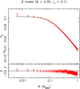
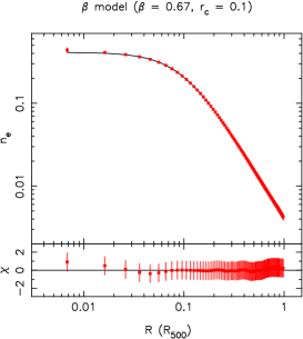
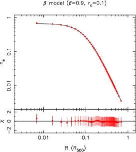
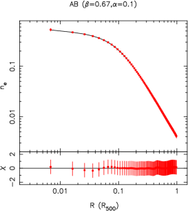
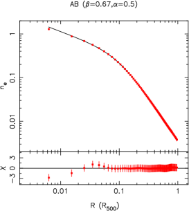
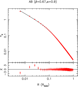
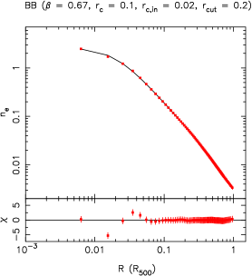
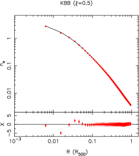
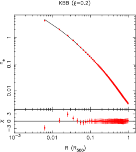
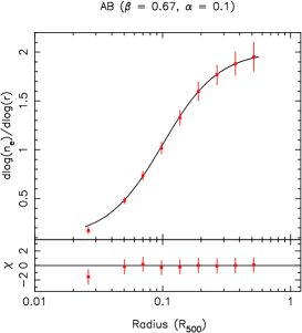
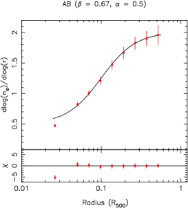
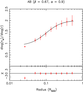
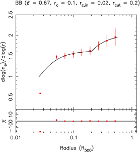
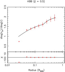
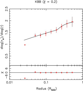
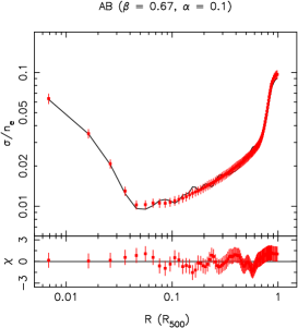
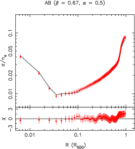
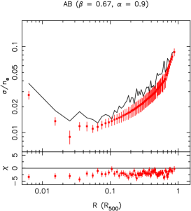
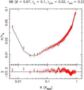
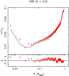
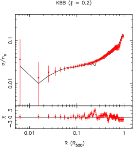
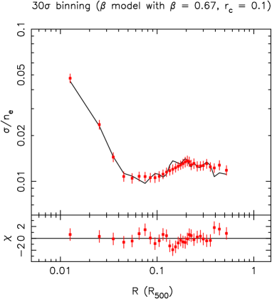
We ran the simulation for each of these profile shapes for several sets of parameters to test the influence of profile shape on code performance. The results are shown in Figure 1. For these tests, the input surface brightness profiles had a global signal-to-noise ratio of 200, representative of a typical observation of a nearby cluster, a total source/background count ratio $R=0.3$, appropriate for this signal-to-noise, and were binned to obtain a signal-to-noise per bin of at least $3\sigma$.

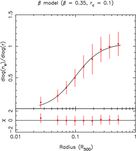
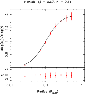
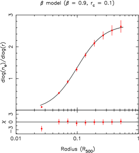
Fig. 1 shows that our deprojection method is not significantly affected by the profile shape: in all cases the input density profile is recovered to a high degree of accuracy. A more quantitative comparison is given in Table 1: the reduced $\chi 2$ values for the mean output density profile compared to the input profile show that there is no significant bias. It appears that the scaling function does have a small effect on the code performance: the BB and KBB models, for which the goodness of fit of the scaling AB model were poorest, have significant residuals in the central few bins. However, the overall agreement between the mean output and input profiles (see Table 1) is still excellent. In Figure 2, we show the $d\log{n_{e}}/d\log{r}$ profiles for each of the models, calculated as described in Section 2.4, compared with the slope of the input density profile, calculated directly from the model. As indicated in Table 1, our method accurately and without bias recovers $d\log{n_{e}}/d\log{r}$ for all tested input density models (although the slope is less well-recovered in the innermost bin for the steepest density profiles).

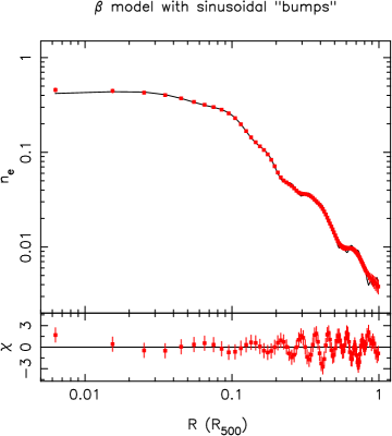
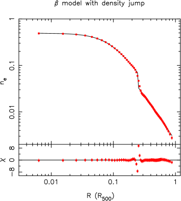
As one of the main strengths of this method is that it retains full information from the surface brightness profile, we also wanted to test its ability to recover information about deviations from a smooth functional form in the input density profile. We therefore simulated density profiles containing sinusoidal modulations superimposed on a $\beta$-model form in order to represent more complex profile behaviour. Figure 3 shows the simulation results for one such profile, which is representative of the “bumpy” profiles that were investigated. Again, the deprojection code recovers extremely well the shape of the “bumps” in the input profile, although they are slightly smoothed, as is evident in the residual plot. We also simulated a profile with a density discontinuity (by reducing the $\beta$ model normalisation by a factor of 2 at a radius of $2.5r_{c}$) such as might be produced by a cold front. Again, the profile is well reproduced, although the output density discontinuity is slightly smoothed compared to the input profile. The slight smoothing effect will be more severe for very narrow, spiked features (as was noted by Bouchet (1995) for his original application of this technique to spectral deconvolution); however, in the case of X-ray surface brightness profiles, such features would not be expected as they are unphysical, so that this is not an important limitation of the code. Although we have demonstrated that radial imhomogeneities in gas distribution are well recovered by our method, it is important to be aware of the inherent limitations of a one-dimensional approach to measuring gas density. Like all methods based on azimuthally symmetric radial surface brightness profiles, our deprojection method does not take into account azimuthal variations or variations along the line-of-sight. Our method could be generalized to ellipsoid shells; however, this would require assumptions about the cluster structure along the line-of-sight. A detailed discussion of the accuracy of 1-D deprojection methods is beyond the scope of this paper.

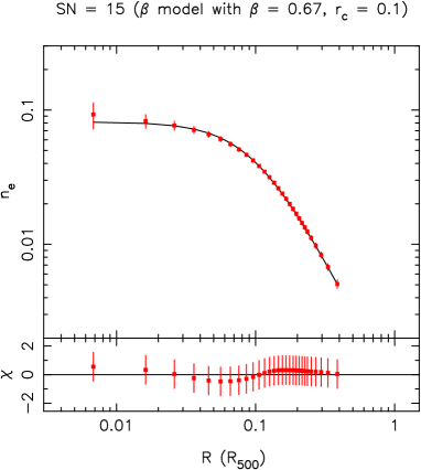
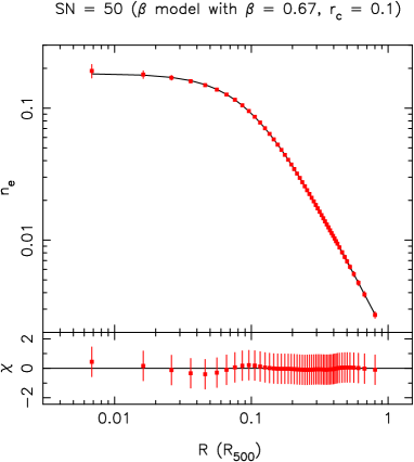
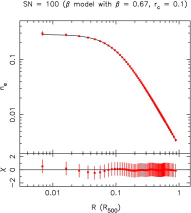
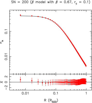
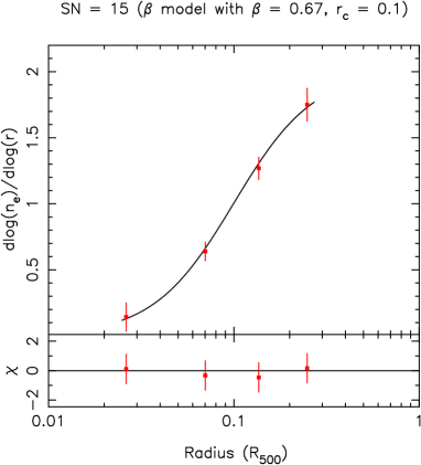
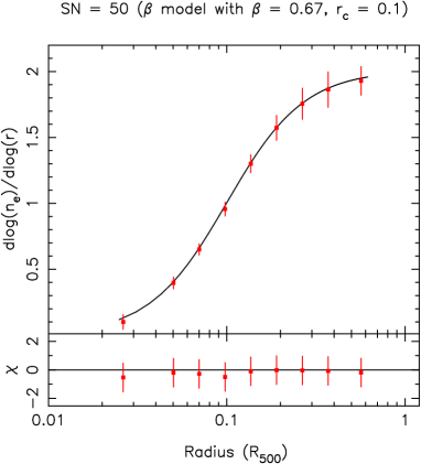
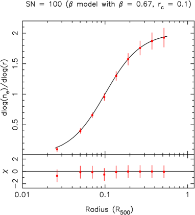
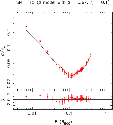
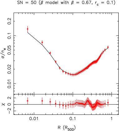
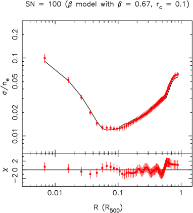
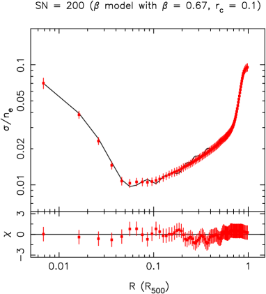
We next used a $\beta$ model profile (for simplicity) to test the effects of global signal-to-noise ratio and choice of binning. We tested $\beta$ model profiles with $\beta=0.67$ (typical of cluster profiles) and $r_{c}=0.1R_{500}$ for global signal-to-noise ratios of 200, 100, 50 and 15, which fully sample the range in data quality seen in observations of nearby and distant clusters. The corresponding total source/background count ratios were 0.3, 1, 2 and 5, respectively, as obtained using the relationship between signal-to-noise and $R$ in the observations. Figure 4 shows the deprojection results for the four choices of global S/N, with goodness of fit information in Table 2. Unsurprisingly, the code performs best for the highest quality data; however, in all cases the input density profile is well recovered, and even at the lowest S/N ratio of 15, the deprojection method performs well ($\chi^{2}$ of 0.1 for 24 d.o.f. for the mean output profile). This is further illustrated by the plots of $d\log{n_{e}}/d\log{r}$ shown in Figure 5.

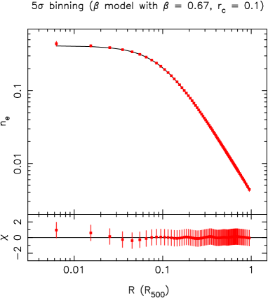
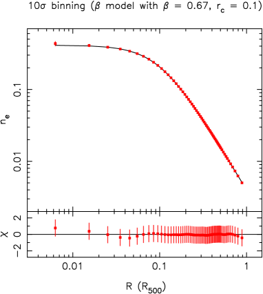
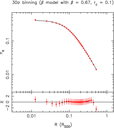
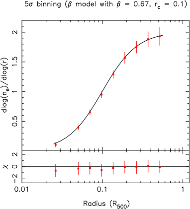
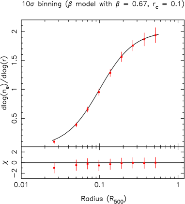
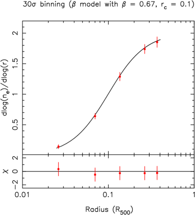
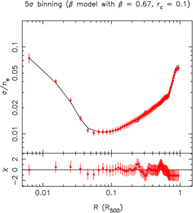
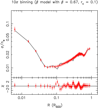
We then tested the effect of binning of the input surface brightness profile on the performance of our method. Using the same $\beta$ model parameters as for the global S/N tests, and a global S/N of 200 again, we tested binning with ratios of 3, 5, 10 and 30$\sigma$ per bin. The deprojection results for these tests are shown in Figure 6, with goodness of fit information in Table 2, and plots of $d\log{n_{e}}/d\log{r}$ in Figure 7. These figures show that the choice of binning does not have an important effect on the recovery of the input density profile.

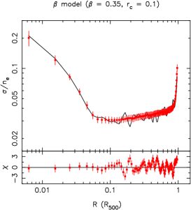
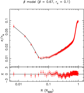
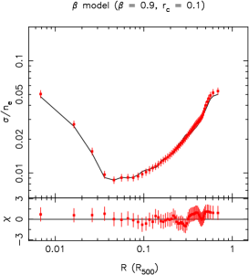
In addition to testing how well the input density profiles were recovered in our simulations, we also tested the accuracy of our error calculation method (described in Section 2.3). The “true” error on the density calculated at a given radius should be given by the standard deviation of the distribution of density values ($\sigma_{n_{e}}$) obtained over the 100 Monte Carlo runs for a given model (indeed, this is precisely the method we are using in the error calculation). We therefore compared the mean errors calculated by our code at each density ($<\sigma_{calc}>$) with the “true” error from the simulated density distribution ($\sigma_{n_{e}}$) to confirm the accuracy of our method. Figure 8 shows a comparison of $<\sigma_{calc}>(r)$ and $\sigma_{n_{e}}(r)$ for a range of models, with Figs. 9 and  10 illustrating the effect of global S/N and choice of binning on the accuracy of error determination. In all cases the errors calculated by the code are reasonably accurate (within 2$\sigma$ of the true error) and generally not biased in any systematic way (although for the steepest AB model there is a slight systematic underestimation, the origin of which is unclear). The accuracy of the error calculations is also shown in Table 1.

Table 1: Code performance for different profile shapes

Model	$\beta$	$r_{c}$	$r_{c,in}$	$r_{cut}$	$\alpha$	$\xi$	$\chi^{2}_{dens}/N_{bins}$	$\chi^{2}_{denserrs}/N_{bins}$	$\chi^{2}_{slope}/N_{bins}$	$\chi^{2}_{slopeerrs}/N_{bins}$
$\beta$	0.67	0.1	–	–	–	–	1.54/55	45.2/55	2.7/54	39.5/54
$\beta$	0.35	0.1	–	–	–	–	23.0/64	76.2/63	4.5/63	52.1/60
$\beta$	0.9	0.1	–	–	–	–	5.5/47	39.2/47	4.2/46	30.7/46
AB	0.67	0.1	–	–	0.1	–	1.02/54	84.2/54	1.1/54	94.0/54
AB	0.67	0.1	–	–	0.5	–	2.65/52	42.5/52	9.2/52	26.5/52
AB	0.67	0.1	–	–	0.9	–	8.46/49	229/48	5.9/49	228/46
BB	0.67	0.1	0.02	0.2	–	–	19.1/49	31.1/49	36.1/49	39.3/49
KBB	0.67	0.1	0.02	0.2	–	0.5	11.8/50	71.9/50	19.4/50	67.0/50
KBB	0.67	0.1	0.02	0.2	–	0.2	2.92/49	56.8/49	5.1/49	39.5/49
bumpy	-	-	-	-	-	-	111.3/91	-	121.4	-
cold front	-	-	-	-	-	-	133.2/69	-	131/69	-

Table 2: Code performance for different global S/N and binning

S/N	$\sigma_{bin}$	$\chi^{2}_{mean}/N_{bins}$	$\chi^{2}_{errs}/N_{bins}$	$\chi^{2}_{slope}/N_{bins}$	$\chi^{2}_{slopeerrs}/N_{bins}$
15	3.0	2.2/24	37.2/24	2.2/23	39.2/23
50	3.0	1.54/42	24.1/42	1.3/41	25.1/41
100	3.0	1.54/55	45.2/55	2.7/54	39.5/54
200	3.0	2.1/71	55.5/71	2.9/70	40.2/70
200	5.0	2.06/45	33.5/45	1.7/44	27.3/44
200	10.0	5.6/33	38.4/33	3.3/32	41.8/32
200	30.0	14.1/17	15.1/17	9.0/17	15.6/17

4 A comparison of XMM-Newton and Chandra gas density profiles using the new method

In the previous section we demonstrated using a range of model density profiles that our deprojection method performs well in a variety of situations. We next decided to carry out a comparison of the Chandra and XMM-Newton density profiles obtained using our method and from analytical models for several clusters for which high quality data exist from both observatories. The purpose of this comparison was both to test the performance of our code on real data and also to test for the first time the consistency of surface brightness and density profiles obtained from the two observatories. The comparison of deprojected XMM-Newton profiles with Chandra profiles will be particularly useful as a test of our PSF-deconvolution method, as the much smaller Chandra PSF means that its effects on the central profile are far less important.

We chose to study three nearby clusters Abell 478, Abell 1413 and Abell 1991, which have recently published observations with XMM-Newton (Pointecouteau et al. 2004, Pratt & Arnaud 2002, 2005) and Chandra (Sun et al. 2003, Vikhlinin et al. 2006).

For Abell 478, we used the XMM-Newton surface brightness profile obtained by Pointecouteau et al. (2004) as input for the deprojection code. The deprojected XMM-Newton density profile was then compared with the analytical model fitted by Pointecouteau et al. (2004) and with the Chandra density profile obtained by Sun et al. (2003). Sun et al. (2003) in fact also used a deprojection method to obtain their profile; their method uses an “onion-skin” technique without regularisation. Figure 11 compares the different profiles for Abell 478. All three profiles are in good agreement, although the deprojected XMM profile is slightly more centrally peaked than the Chandra profile.

Figure 11: Comparison of XMM and Chandra profiles for Abell 478 with the XMM profile obtained with our method (+ symbols, the best-fitting XMM model of Pointecouteau et al. (2004) (dashed line), and the Chandra profile of Sun et al. (2003) (dotted line).

We used the XMM-Newton surface brightness profile of Pratt & Arnaud (2002) for Abell 1413 as input for the deprojection code. In this case we compared with the best fitting analytical models of Pratt & Arnaud (the ‘KBB’ model) (XMM) and of Vikhlinin et al. (2006) (Chandra), which consisted of a $\beta$ model multiplied by a polytropic model. Figure 12 compares the different density profiles for Abell 1413. Again, all three density profiles are in good agreement; however, in this case the model obtained from our deprojection method is in better agreement with the Chandra profiles in the central regions than the XMM analytical model, which fails to reproduce the central cuspiness measured by Chandra.

For Abell 1991, we used the XMM-Newton profile of Pratt & Arnaud (2005) as input for the deprojection code, and compared the output density profile with their analytical model (a sum of two $\beta$ models) and with the best-fitting model to the Chandra data of Vikhlinin et al. (2006) (with the same functional form as for Abell 1413, but with an additional second $\beta$-model component). The results are shown in Figure 13. In this case, the two profiles obtained from the XMM-Newton data are in good agreement, but both significantly less centrally peaked than the Chandra profile. The slope of the Chandra profile is also slightly steeper.

Figure 12: Comparison of XMM and Chandra profiles for Abell 1413 with the XMM profile obtained with our method (+ symbols), the best-fitting XMM model of Pratt & Arnaud (2002) (dashed line), and the Chandra profile of Vikhlinin et al. (2006) (dotted line).

Figure 13: Comparison of XMM and Chandra profiles for Abell 1991 with the XMM profile obtained with our method (+ symbols), the best-fitting XMM model of Pratt & Arnaud (2005) (dashed line), and the Chandra profile of Vikhlinin et al. (2006) (dotted line).

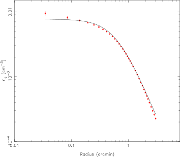
Finally, we also decided to test the code on a more distant cluster observed by XMM-Newton, CL0016+16 ($z=0.5455$). Figure 14 shows our deprojected density profile with the best-fitting $\beta$-model profile of Worrall & Birkinshaw (2003) both from the XMM-Newton observation. The profiles are in good agreement, except at the centre, where Worrall & Birkinshaw’s model fit had systematic residuals, and in the outermost bins, where our method identifies a steepening at large radius that could not be taken into account by the $\beta$-model fit.

Figure 14: Comparison of XMM profile for CL0016+16 with the XMM profile obtained with our method shown in red and the best-fitting XMM model of Worrall & Birkinshaw (2003) in black.

5 A comparison of mass profiles

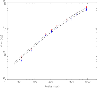
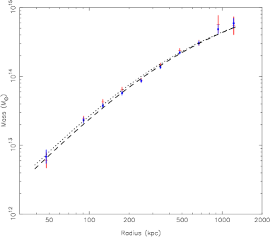
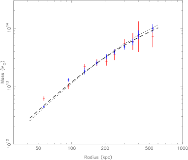
In addition to comparing the gas density profiles obtained from Chandra and XMM-Newton cluster observations, as discussed in the previous section, we also compared the mass profiles of Abell 478, Abell 1413 and Abell 1991 obtained from the XMM-Newton observations via the two methods of deprojection and model fitting to obtain $d\log(n_{e})/d\log(r)$. For both sets of density slope profiles, we used the same temperature profiles, those of Pointecouteau et al. (2004), Pratt & Arnaud (2002) and (2005), respectively, for Abell 478, Abell 1413 and Abell 1991, to calculate a total mass profile. Fig. 15 shows the mass profiles for all three clusters. In all three cases the two methods of analysis of the XMM-Newton data obtain similar results. In general (and particularly for Abell 1991), the XMM-Newton profiles obtained by model fitting are smoother than those obtained via the deprojection method, which is not surprising; however, the best-fitting NFW model fits for the new method are consist within 1$\sigma$ with those reported in the original XMM-Newton analysis papers for each cluster.

6 Conclusions

We have described a method for obtaining gas density profiles from X-ray surface brightness profiles of galaxy clusters, with the aim of improving constraints on the entropy and total mass distributions of clusters. We first showed using simulated profiles that this method performs well in a range of conditions:

• The effect of the shape of the density profile was tested using four models: the $\beta$ model, AB model, KBB model, BB model, as well as for profiles with deviations from a smooth shape. We found that in all cases the agreement between the output density profile and the model was good, with slightly poorer performance in the central regions for the KBB and BB models, due to the choice of an AB model as a scaling function.

• The global signal-to-noise of the input profiles does affect the accuracy of the output density profiles, with poorer quality data giving less accurate results; however, this effect was fairly small, and a good agreement ($\chi^{2}$ of 36/24) was obtained for a S/N of 15, corresponding to a profile containing $\sim 2500$ net counts.

• The profile binning did not appear to have an important effect on the accurate recovery of the input density profile.

We then tested the code performance on real XMM-Newton data for four clusters: three nearby clusters with published Chandra gas density profiles, and one distant cluster. We found that our method resulted in gas density profiles in better agreement with the higher resolution Chandra profiles. We also found that our method performed well in the case of the distant cluster, CL0016+16, reproducing a central excess and change of slope at large radii that could not be taken into account using a $\beta$-model fit. Finally we demonstrated that the mass profiles obtained from our gas density profiles are consistent with those obtained from other methods. We therefore find that our method is suitable for obtaining gas density profiles both from high signal-to-noise observations of nearby clusters and also for distant clusters. This model-independent inversion method will be extremely useful as a consistent and reliable means of obtaining gas density profiles (and subsequently entropy and mass profiles) for ongoing studies of large, unbiased samples of nearby and distant clusters. The deprojection code is available on request to the authors.

Figure 15: Mass profile comparison for Abell 478 (top left), Abell 1413 (top right) and Abell 1991 (bottom). In all cases, red + symbols indicate the XMM mass profile obtained by deprojection, blue squares the XMM mass profile obtained by fitting a model to the surface brightness distribution (taken from Pointecouteau et al. 2004, Pratt & Arnaud 2002, and 2005, respectively). Dashed lines indicate NFW fits to the profiles using deprojection, and dotted lines best fits to the profiles using analytic density profiles.

We would like to thank the referee for useful comments.

References

- (1) Arnaud, M., 2005, in ”Background Microwave Radiation and Intracluster Cosmology”, eds. F. Melchiorri & Y. Rephaeli, IOS Press, astro-ph/0508159
- (2) Arnaud, M., Pointecouteau, E., Pratt, G.W., 2005, A&A, 441, 893
- (3) Bouchet, L., 1995, A&AS, 113, 167
- (4) David, L.P., Nulsen, P.E.J., McNamara, B.R., Forman, W., Jone,s C., Ponman, T., Robertson, B., Wise, M., 2001, ApJ, 557, 546
- (5) Fabian, A.C., Hu, E.M., Cowie, L.L., Grindlay, J., 1981, ApJ, 248, 47
- (6) Ghizzardi, S., XMM-SOC-CAL-TN-0022, available from http://xmm.vilspa.esa.es
- (7) Kay, S.T., Thomas, P.A., Jenkins, A., Pearce, F.R., 2004, MNRAS, 355, 1091
- (8) Kriss, G.A., Cioffi, D.F., Canizares, C.R., 1983, ApJ, 272, 439
- (9) McLaughlin, D.E., 1999, AJ, 117, 2398
- (10) Neumann, D.M., Arnaud, M., 1999, A&A, 348, 711
- (11) Phillips, D., L., 1962, J. Assoc. Comp. Mach., 9, 84
- (12) Pointecouteau, E., Arnaud, M., Kaastra, J., de Plaa, J., 2004, A&A, 423, 33
- (13) Pointecouteau, E., Arnaud, M., Pratt, G.W., 2005, A&A, 435, 1
- (14) Ponman, T.J., Cannon, D.B., Navarro, J.F., 1999, Nature, 397, 135
- (15) Ponman, T.J., Sanderson, A.J.R., Finoguenov, A., 2003, MNRAS, 343, 331
- (16) Pratt, G.W., Arnaud, M., 2002, A&A, 394, 375
- (17) Pratt, G.W., Arnaud, M., 2005, A&A, 429, 791
- (18) Pratt, G.W., Arnaud, M., Pointecouteau, E., 2006, A&A, 426, 429
- (19) Sun, M., Jones, C., Murray, S.S., Allen, S.W., Fabian, A.C., Edge, A.C., 2003, ApJ, 587, 619
- (20) Towmey, S., 1963, J. Assoc. Comp. Mach., 10, 97
- (21) Vikhlinin, A., Kravtsov, A., Froman, W., Jones, C., Markevitch, M., Murray, S.S., Van Speybroeck, L., 2006, ApJ, 640, 691
- (22) Voit, G.M., 2005, Rev.Mod. Phys., 77, 207
- (23) Wahba, G., 1978, Journal of the Royal Statistical Society, B3, 364
- (24) White, D.A., Jones, C., Forman, W., 1997, MNRAS, 292, 419
- (25) Worrall, D.M., Birkinshaw, M., 2003, MNRAS, 340, 1261