Self-induced conversion in dense neutrino gases: Pendulum in flavour space

Abstract

Neutrino-neutrino interactions can lead to collective flavour conversion effects in supernovae and in the early universe. We demonstrate that the case of “bipolar” oscillations, where a dense gas of neutrinos and antineutrinos in equal numbers completely converts from one flavour to another even if the mixing angle is small, is equivalent to a pendulum in flavour space. Bipolar flavour conversion corresponds to the swinging of the pendulum, which begins in an unstable upright position (the initial flavour), and passes through momentarily the vertically downward position (the other flavour) in the course of its motion. The time scale to complete one cycle of oscillation depends logarithmically on the vacuum mixing angle. Likewise, the presence of an ordinary medium can be shown analytically to contribute to a logarithmic increase in the bipolar conversion period. We further find that a more complex (and realistic) system of unequal numbers of neutrinos and antineutrinos is analogous to a spinning top subject to a torque. This analogy easily explains how such a system can oscillate in both the bipolar and the synchronised mode, depending on the neutrino density and the size of the neutrino-antineutrino asymmetry. Our simple model applies strictly only to isotropic neutrino gasses. In more general cases, and especially for neutrinos streaming from a supernova core, different modes couple to each other with unequal strength, an effect that can lead to kinematical decoherence in flavour space rather than collective oscillations. The exact circumstances under which collective oscillations occur in non-isotropic media remain to be understood.

I Introduction

The “refractive index” caused by a medium has a strong impact on neutrino flavour oscillations Wolfenstein:1977ue ; Mikheev:1986gs ; Mikheev:1986wj ; Fuller1987 ; Notzold:1987ik ; Kuo:1989qe . This matter effect is a standard ingredient for neutrino oscillations in laboratory experiments and in astrophysical environments. However, when neutrinos themselves form a significant “background medium” as in the early universe or in core-collapse supernovae, the oscillation equations become nonlinear, sometimes resulting in surprising collective phenomena. Based on Pantaleone’s key observation that neutrinos as a background medium produce a flavour off-diagonal refractive index Pantaleone:1992eq , the behaviour of dense neutrino gases was investigated in a series of papers by Samuel, Kostelecký and Pantaleone Samuel:1993uw ; Kostelecky:1994ys ; Kostelecky:1993yt ; Kostelecky:1993dm ; Kostelecky:1995dt ; Kostelecky:1995xc ; Samuel:1996ri ; Kostelecky:1996bs ; Pantaleone:1998xi . Two classes of collective effects were identified in these papers: we shall call them “synchronised” and “bipolar” oscillations, respectively.

Synchronised oscillations occur when the neutrino-neutrino interaction potential is large compared to the ordinary oscillation frequencies in vacuum or in a medium, and a sufficiently large asymmetry exists between the neutrino and antineutrino distributions. As a result, all neutrinos and antineutrinos oscillate with the same frequency that is a certain average of the ordinary oscillation frequencies. In the spin-precession analogy of flavour oscillations, the flavour polarisation vectors of all neutrino modes form one big spin that precesses in a weak “external magnetic field.” This big spin is held together by the strong “internal magnetic field” formed in flavour space by the strong neutrino-neutrino interaction Pastor:2001iu . Various qualitative and quantitative aspects of synchronised oscillations and applications to neutrino flavour oscillations in the early universe Lunardini:2000fy ; Dolgov:2002ab ; Wong:2002fa ; Abazajian:2002qx were studied a few years ago, motivated by the question if neutrinos with chemical potentials reach flavour equilibrium in the early universe before the epoch of big-bang nucleosynthesis.

Much less attention has been paid to bipolar flavour conversions, but very recently it has been recognised that this peculiar phenomenon likely plays a crucial role for supernova neutrino oscillations Duan:2005cp ; Duan:2006an ; Duan:2006jv . In the simplest case, bipolar oscillations occur in a dense gas of equal numbers of neutrinos and antineutrinos of the same flavour. For a suitable mass hierarchy, even a small mixing angle can cause a complete conversion of both neutrinos and antineutrinos to the other flavour. We stress that a non-vanishing vacuum mixing angle is pivotal; bipolar oscillations, although a quasi self-induced effect, will not occur if the vacuum mixing angle strictly vanishes.

The relevant conditions for bipolar conversions probably occur for neutrinos streaming off a collapsed supernova core where one expects a hierarchy of average energies $\langle E_{\nu_{e}}\rangle<\langle E_{\bar{\nu}_{e}}\rangle<\langle E_{\nu_{x}}\rangle$ with $\nu_{x}=\nu_{\mu},\bar{\nu}_{\mu},\nu_{\tau},\bar{\nu}_{\tau}$ Keil:2002in . Assuming equal luminosities for all species, the number flux of, say, $\nu_{\mu}$ and $\bar{\nu}_{\mu}$ is each smaller than that of $\nu_{e}$ and $\bar{\nu}_{e}$ respectively. For the inverted mass hierarchy one would then expect bipolar oscillations driven by the “atmospheric” neutrino mass difference and the small mixing angle $\Theta_{13}$.

Bipolar flavour conversion occurs when the neutrino-neutrino interaction energy, $\mu=\sqrt{2}G_{\rm F}n_{\nu}$, exceeds a typical vacuum oscillation frequency $\omega=\Delta m^{2}/2E$. Furthermore, the neutrino-antineutrino asymmetry must not be too large in a sense to be quantified later. Once these conditions are met, bipolar oscillations take place for astonishingly small values of the mixing angle and are nearly unaffected by the presence of an ordinary background medium, even if it is much denser than the neutrino gas Duan:2005cp . These oscillations are also unrelated to a Mikheyev-Smirnov-Wolfenstein (MSW) resonance of the ordinary background medium.

The notion of “bipolar oscillations” originates from the claimed numerical observation that the flavour polarisation vectors of all neutrinos and of all antineutrinos align together to form two “block spins” that evolve separately. Indeed, the analytic descriptions of Refs. Kostelecky:1995dt ; Samuel:1996ri were based on the study of a system of one neutrino and one antineutrino polarisation vector that were taken to represent, respectively, the complete ensemble of neutrinos and antineutrinos. We find that this description of bipolar oscillations is incorrect and actually has never been explicitly demonstrated in the literature. In fact, each mode of the neutrino and antineutrino ensemble evolves differently and the term “bipolar” is a misnomer. On the other hand, the behaviour is bipolar in the sense that neutrinos and antineutrinos oscillate in “opposite directions” and thus form two separate cohorts, even if they do not form two block spins. Therefore, we use the term “bipolar” to describe this collective phenomenon.

The newly recognised role of bipolar oscillations represents a change of paradigm for supernova neutrino oscillations. Inspired by these exciting developments we turn to an analytic study of bipolar oscillations with the aim of providing a simple qualitative and quantitative understanding of the salient features of this puzzling effect. Analytic solutions for certain cases have already been provided in the literature Kostelecky:1995dt ; Samuel:1996ri . However, a judicious choice of variables enables us to write the equations of motion in the form of an ordinary pendulum. This picture allows one to grasp the salient features of the bipolar phenomenon at a single glance. Moreover, it allows one to calculate explicitly the dependence of the bipolar oscillation period on the vacuum mixing angle and on the density of an ordinary background medium.

When the fluxes of neutrinos and antineutrinos are not equal (as expected for supernova neutrinos), the equations for the flavour pendulum remain the same, but the asymmetric initial conditions imply the presence of an inner angular momentum (i.e., spin) of the pendulum: the system is equivalent to a spinning top subject to a torque. If the top is not spinning, we simply recover the motion of an ordinary spherical pendulum (i.e., bipolar behaviour of a symmetric $\nu$-$\bar{\nu}$ system). Otherwise the motion is more complicated. If the spin is sufficiently large, the top precesses in the force field exerting the torque (i.e., synchronised oscillations). If the spin is too small, the top wobbles or even completely turns over (i.e., bipolar behaviour of an asymmetric system).

In the most general case, however, different neutrino modes have different energies and, in a non-isotropic medium such as that encountered by neutrinos streaming off a supernova core, couple to each other with different strengths (“multi-angle case”). In this situation kinematical decoherence rather than collective oscillations can obtain and is an unavoidable outcome certainly in the simplest system of equal numbers of neutrinos and antineutrinos. However, in the more realistic case of unequal neutrino and antineutrino fluxes in conjunction with a slowly varying effective neutrino density, collective oscillations often still obtain. The exact criteria that determine if kinematical decoherence or collective oscillations occur remain to be understood.

We begin in Sec. II with the simplest bipolar system consisting of one polarisation vector for the neutrinos and one for the antineutrinos and establish the equivalence to a flavour pendulum. We then study analytically the impact of an ordinary background medium in Sec. III. In Sec. IV we allow the neutrino density to vary and show that this effect is crucial for the nearly complete flavour conversion in supernovae. In Sec. V we consider a system with an initial $\nu$-$\bar{\nu}$ asymmetry and show its equivalence to a spinning top subject to a torque. We apply our insights to explain the salient features of flavour conversion of the neutrinos streaming off a supernova core. In Sec. VI we consider a system of many modes and discuss the conditions under which it is equivalent to the simple bipolar system. In Sec. VII we discuss the possibility of flavour conversion initiated by quantum fluctuations, in the absence of flavour mixing. A summary of our findings is given in Sec. VIII.

II Basic Bipolar System

II.1 Equations of motion

We begin with the simplest bipolar system initially composed of equal densities of pure $\nu_{e}$ and $\bar{\nu}_{e}$. All of them are taken to have equal energies so that the vacuum oscillation frequencies are the same for all modes. We describe the flavour content of these ensembles with polarisation vectors in flavour space ${\bf P}$ and $\bar{\bf P}$, where overbarred quantities refer to antiparticles here and henceforth. Without loss of generality we take these vectors to have unit length. As usual, the $z$-component of the polarisation vector represents the flavour content of the ensemble, i.e., the survival probability of $\nu_{e}$ at time $t$ is $\frac{1}{2}[1+P_{z}(t)]$. We take the positive $z$ direction to represent the electron flavour so that both ${\bf P}$ and $\bar{\bf P}$ are initially unit vectors in the $z$-direction.

In the absence of ordinary matter the general equations of motion Eq. (A.2) are

$$\partial_{t}{\bf P} = \left[+\omega{\bf B}+\mu\left({\bf P}-\bar{\bf P}\right)\right]\times{\bf P}\,,$$

$$\partial_{t}\bar{\bf P} = \left[-\omega{\bf B}+\mu\left({\bf P}-\bar{\bf P}\right)\right]\times\bar{\bf P}\,,$$ (1)

where $\omega>0$ is the vacuum oscillation frequency, $\mu=\sqrt{2}G_{F}n_{\nu}$ represents the strength of the $\nu$-$\nu$ interaction, i.e., the density of the neutrino gas, and ${\bf B}=(\sin 2\theta_{0},0,-\cos 2\theta_{0})$ with vacuum mixing angle $\theta_{0}$.

A mixing angle close to zero corresponds to the normal mass hierarchy in which $\nu_{e}$ is essentially identical with the lower mass state, while $\theta_{0}$ near $\pi/2$ corresponds to the inverted hierarchy with $\nu_{e}$ residing largely in the heavier mass state. In the latter case we will also use the notation

$$\tilde{\theta}_{0}=\pi/2-\theta_{0}\,.$$ (2)

Therefore, whenever $\tilde{\theta}_{0}$ appears as a small quantity it signifies directly that we are in an inverted mass situation. Alternatively, one could restrict the vacuum mixing angle to $0\leq\theta_{0}\leq\pi/4$ and switch to the inverted hierarchy with the replacement $\omega\to-\omega$. However, in our treatment it is more natural to keep $\omega$ always positive and extend the range of mixing angles to $0\leq\theta_{0}\leq\pi/2$.

In order to illustrate the phenomena we wish to study we show in Fig. 1 the evolution of $P_{z}$ for a vacuum mixing angle near $\pi/2$, corresponding to an inverted mass hierarchy. At first ${\bf P}$ hardly moves at all, but after some time it flips almost completely. Therefore, even a very small mixing angle leads to complete flavour conversion. Of course, this simple system is periodic so that the motion then reverses itself. The behaviour of $\bar{P}_{z}$ is identical to that of $P_{z}$. In other words, both $\nu_{e}$ and $\bar{\nu}_{e}$ convert simultaneously to $\nu_{\mu}$ and $\bar{\nu}_{\mu}$.

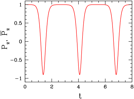
Figure 1: Evolution of $P_{z}$ and $\bar{P}_{z}$ for the system of equations Eq. (II.1) with $\tilde{\theta}_{0}=0.01$ (i.e., inverted hierarchy), $\omega=1$, and strong neutrino-neutrino interaction $\mu=10$. (This figure is essentially identical to Fig. 3 of Ref. Pastor:2001iu .)

This evolution can be understood from Eq. (II.1). Initially the difference of the polarisation vectors

$${\bf D}={\bf P}-\bar{\bf P}$$ (3)

vanishes so that there is no neutrino-neutrino effect. When the polarisation vectors ${\bf P}$ and $\bar{\bf P}$ begin to precess in opposite directions around ${\bf B}$, a non-zero ${\bf D}$ develops in the $y$-direction orthogonal to ${\bf B}$. Both ${\bf P}$ and $\bar{\bf P}$ then tilt around ${\bf D}$, leading to a complete flavour reversal (inverted hierarchy) or to small oscillations (normal hierarchy).

Observe that ${\bf P}$ and $\bar{\bf P}$ behave symmetrically and their $z$-components develop identically. This suggests that instead of these polarisation vectors one should use their sum and difference vectors as independent variables, i.e., ${\bf D}$ as defined in Eq. (3), and

$${\bf S}={\bf P}+\bar{\bf P}\,.$$ (4)

The $z$-component of ${\bf S}$ quantifies the flavour content of the combined $\nu_{e}$ and $\bar{\nu}_{e}$ ensemble. The equations of motion for the ${\bf S}$ and ${\bf D}$ vectors are

$$\dot{\bf S} = \omega{\bf B}\times{\bf D}+\mu{\bf D}\times{\bf S}\,,$$

$$\dot{\bf D} = \omega{\bf B}\times{\bf S}\,.$$ (5)

The first line of Eq. (II.1) suggests yet another vector to describe the ensemble,

$${\bf Q}={\bf S}-\frac{\omega}{\mu}{\bf B}\,.$$ (6)

For strong neutrino-neutrino interactions ($\mu/\omega\gg 1$) we can think of ${\bf Q}$ as identical to ${\bf S}$.

Since $\dot{\bf B}=0$, it follows that $\dot{\bf S}=\dot{\bf Q}$. With ${\bf B}\times{\bf Q}={\bf B}\times{\bf S}$, the equations of motion are now

$$\dot{\bf Q} = \mu{\bf D}\times{\bf Q}\,,$$

$$\dot{\bf D} = \omega{\bf B}\times{\bf Q}\,.$$ (7)

Clearly, the length of ${\bf Q}$ is conserved and stays at its initial value

$$Q=|{\bf Q}|=\left[4+\left(\frac{\omega}{\mu}\right)^{2}+4\,\frac{\omega}{\mu}\cos 2\theta_{0}\right]^{1/2}\,,$$ (8)

where we have used $|{\bf B}|^{2}=1$, and the initial values $|{\bf S}|^{2}=4$ and ${\bf B}\cdot{\bf S}=-2\cos 2\theta_{0}$.

II.2 Spherical pendulum

The vector ${\bf Q}$ in flavour space plays the role of a spherical pendulum in that its length is conserved so that it can move only on a sphere of radius $Q$. In this picture, the role of the different quantities is most easily understood if we consider the total energy of the system,

$$H=\omega{\bf B}\cdot{\bf Q}+\frac{\mu}{2}{\bf D}^{2}\,,$$ (9)

up to a constant. The first term is the potential energy of the pendulum in a homogeneous force field represented by $\omega{\bf B}$. The second term is the kinetic energy, with ${\bf D}$ playing the role of the pendulum’s orbital angular momentum. Observing that ${\bf D}\cdot{\bf Q}=-(\omega/\mu){\bf D}\cdot{\bf B}$ is constant due to Eq. (II.1) and thus zero in our case ${\bf D}(0)=0$, the first line in Eq. (II.1) implies

$${\bf D}=\frac{1}{\mu}\,\frac{{\bf Q}\times\dot{\bf Q}}{Q^{2}}\,,$$ (10)

and hence ${\bf D}^{2}=\mu^{-2}\,\dot{\bf Q}^{2}/{Q^{2}}$. The scale of the potential energy is set by the vacuum neutrino oscillation frequency $\omega$, whereas $I=\mu^{-1}$ is to be identified with the moment of inertia. The latter should be compared with $I=m\ell^{2}$ for an ordinary mass suspended by a string of length $\ell$. The role of inertia in the pendulum analogy is played by the inverse strength of neutrino-neutrino interaction!

II.3 Plane pendulum

Our initial conditions ${\bf P}(0)=\bar{\bf P}(0)=(0,0,1)$ imply ${\bf D}(0)=0$. The pendulum’s subsequent oscillations are confined in a plane defined by ${\bf B}$ and the $z$-axis. Therefore, the problem reduces to solving for the motion of the tilt angle $\varphi$ of ${\bf Q}$ relative to the $z$-axis. Writing ${\bf Q}=Q\,(\sin\varphi,0,\cos\varphi)$, we find

$$\dot{\varphi} = \mu D\,,$$

$$\dot{D} = -\omega Q\sin(\varphi+2\theta_{0})\,.$$ (11)

Equation (II.3) can be further simplified to

$$\ddot{\varphi}=-\kappa^{2}\,\sin(\varphi+2\theta_{0})\,,$$ (12)

where

$$\kappa^{2}=\omega\mu Q\,.$$ (13)

The inverse of $\kappa$ is the characteristic time scale for the bipolar evolution. In the limit of strong neutrino-neutrino coupling, $Q\approx 2$ and hence $\kappa\approx\sqrt{2\omega\mu}$. In the opposite limit ($\mu\ll\omega$), we have $Q\approx\omega/\mu$ so that $\kappa\approx\omega$. In this latter case the characteristic frequency of the system is the vacuum oscillation frequency $\omega$, and ${\bf P}$ and $\bar{\bf P}$ oscillate independently.

The equations of motion (II.3) follow directly from the classical Hamiltonian for a simple pendulum

$$H(\varphi,D)=\frac{\kappa^{2}}{\mu}\bigl{[}1-\cos(\varphi+2\theta_{0})\bigr{]}+\frac{1}{2}\,\mu\,D^{2}\,,$$ (14)

where $\varphi$ is a coordinate and $D$ its canonically conjugate momentum. Indeed, the equations (II.3) are but $\dot{\varphi}=\partial H/\partial D$ and $\dot{D}=-\partial H/\partial\varphi$.

Assuming a small vacuum mixing angle $\theta_{0}$ and a small excursion angle $\varphi$ of the pendulum, the potential can be expanded

$$V(\varphi) = \kappa^{2}\,\left[1-\cos(\varphi+2\theta_{0})\right]$$ (15)

$$= \frac{\kappa^{2}}{2}\,\left(\varphi+2\theta_{0}\right)^{2}+\ldots\,.$$

In this case the system is equivalent to a harmonic oscillator with frequency $\kappa$. On the other hand, for angles near $\pi$ so that $|\varphi+2\theta_{0}-\pi|\ll 1$, we get the same expansion but with a negative sign; the system corresponds to an inverted harmonic oscillator.

II.4 Bipolar flavour conversion

II.4.1 Normal hierarchy

Consider the small mixing limit in the normal hierarchy. Here, the initial condition $\varphi(0)\approx-(\omega/\mu Q)\ 2\theta_{0}\geq-2\theta_{0}$ puts $\varphi$ near the minimum of the potential $V(\varphi)$ at $t=0$. Since $\dot{\varphi}(0)=0$, the system remains trapped inside the cosine potential well, oscillating about the minimum $\varphi_{\rm min}=-2\theta_{0}$ with amplitude $(1-\omega/\mu Q)\ 2\theta_{0}$ and frequency $\kappa$. In terms of $P_{z}$ and $\bar{P}_{z}$, any departure from the initial $P_{z}=\bar{P}_{z}=1$ is at most second order in $\theta_{0}$. No dip features develop in this scenario.

II.4.2 Inverted hierarchy with arbitrary $\mu$

Using the relation $\tilde{\theta}_{0}=\pi/2-\theta_{0}$, the potential (15) can be written as

$$V(\varphi) = \kappa^{2}\,\left[1+\cos(\varphi-2\tilde{\theta}_{0})\right]$$ (16)

$$= -\frac{\kappa^{2}}{2}\,\left(\varphi-2\tilde{\theta}_{0}\right)^{2}+\ldots\,$$

in the inverted hierarchy. Depending on the strength of the neutrino-neutrino interactions (i.e., the ratio $\mu/\omega$), $\varphi$ can take on a range of initial values from $\varphi(0)\approx 0$ to $2\tilde{\theta}_{0}-\pi$ in the small $\tilde{\theta}_{0}$ limit. In other words, the evolution of the system begins with $\varphi$ sitting near the maximum of the potential $V(\varphi)$ if $\mu/\omega\geq 1$, or, for smaller values of $\mu/\omega$, somewhere further down the slope.

Since $\dot{\varphi}(0)=0$, the form of the potential $V(\varphi)$ guarantees that $\varphi$ always rolls to the minimum $\varphi_{\rm min}\approx-\pi$ in the small $\tilde{\theta}_{0}$ limit. Evaluating for $P_{z}$ and $\bar{P}_{z}$ at $\varphi=\varphi_{\rm min}$, one finds

$$P_{z}|_{\varphi_{\rm min}}=\bar{P}_{z}|_{\varphi_{\rm min}}\approx\left\{\begin{array}[]{ll}\omega/\mu-1,&\qquad\omega<2\mu,\\ 1,&\qquad\omega\geq 2\mu.\end{array}\right.\,$$ (17)

Thus complete flavour conversion, i.e., $P_{z}=\bar{P}_{z}=-1$, is only possible in the strong neutrino-neutrino coupling limit $\mu/\omega\gg 1$. A partial conversion can be achieved for comparable $\mu$ and $\omega$. No conversion occurs for $\omega\geq 2\mu$, which remains always in the small oscillations regime.

II.4.3 Inverted hierarchy with $\mu\geq\omega$

We now focus on $\mu/\omega\geq 1$. The initial condition $\varphi(0)\approx-(\omega/\mu Q)\ 2\tilde{\theta}_{0}$ puts $\varphi$ near the maximum of the potential $V(\varphi)$ at $t=0$. Since $\dot{\varphi}(0)=0$, and $\varphi(0)$ and $2\tilde{\theta}_{0}$ are both small, the motion of $\varphi$ begins slowly, which explains the long plateau phases between dips in Fig. 1. The dips themselves correspond to the crossing of the anharmonic potential once $\varphi$ grows to the order unity. The duration of the dips is fixed by the crossing time of the anharmonic potential and thus is of order $\kappa^{-1}$. The duration of the plateau, on the other hand, is determined by the smallness of the mixing angle $\tilde{\theta}_{0}$. If $\tilde{\theta}_{0}$ is exactly zero, i.e., no mixing, then there is no motion and $\varphi$ sits at the exact maximum of the potential forever.

In order to estimate the time it takes for the polarisation vectors to flip in the small $\tilde{\theta}_{0}$ limit, we return to the equation of motion for this case,

$$\ddot{\varphi}=\kappa^{2}\sin(\varphi-2\tilde{\theta}_{0}),$$ (18)

with $\tilde{\theta}_{0}\ll 1$. As long as $\varphi$ is small this is equivalent to

$$\ddot{\varphi}=\kappa^{2}(\varphi-2\tilde{\theta}_{0})\,.$$ (19)

Using the initial conditions $\varphi(0)=-(\omega/\mu Q)\ 2\tilde{\theta}_{0}$ and $\dot{\varphi}(0)=0$, this equation is solved by

$$\varphi(t)=2\tilde{\theta}_{0}\left[1-\left(1+\frac{\omega}{\mu Q}\right)\cosh(\kappa t)\right]\,.$$ (20)

Initially $\varphi(t)-\varphi(0)=-\tilde{\theta}_{0}(1+\omega/\mu Q)(\kappa t)^{2}$, but at $t$ of order $\kappa^{-1}$ turns to exponential growth when $\varphi$ has become of order $\tilde{\theta}_{0}$. Therefore, the time it takes for $\varphi$ to grow to order unity, or equivalently, the half period of the bipolar motion is

$$\tau_{\rm bipolar}\approx-\kappa^{-1}\ln[\tilde{\theta}_{0}\ (1+\omega/\mu Q)]\,.$$ (21)

Therefore, the duration of the plateau phases in Fig. 1 or the time between dips scales logarithmically with the small vacuum mixing angle.

II.5 Which mass hierarchy?

We demonstrated that, assuming small mixing, complete flavour conversion occurs for the inverted mass hierarchy, while small oscillations occur for the normal hierarchy. However, this applies only if the initial ensemble consists of $\nu_{e}$ and $\bar{\nu}_{e}$. If the initial ensemble had consisted instead of $\nu_{\mu}$ and $\bar{\nu}_{\mu}$, then the situation would be reversed so that large flavour conversions would occur for the normal hierarchy. Put another way, the unstable case is when the initial ensemble consists of that flavour which is dominated by the heavier mass eigenstate. This symmetry between the neutrino flavours is an important difference to flavour conversion caused by the MSW effect that occurs for the normal mass hierarchy independently of the flavour of the initial state.

II.6 Which flavour conversion?

We have used the term “flavour conversion” loosely to describe the simultaneous conversion of equal numbers of $\nu_{e}$ and $\bar{\nu}_{e}$ to equal numbers of $\nu_{\mu}$ and $\bar{\nu}_{\mu}$. Of course, the net flavour lepton number of the initial state vanishes and remains so at all times. Therefore, the “conversion” we are considering in the bipolar context does not violate flavour lepton number, but, rather, we should think of it as a coherent pair process of the form $\nu_{e}\bar{\nu}_{e}\to\nu_{\mu}\bar{\nu}_{\mu}$.

If the initial system is asymmetric with a net electron lepton number, i.e., ${\bf P}$ and $\bar{\bf P}$ are not initially identical, this difference is quantified by our vector ${\bf D}$, whose projection in the $z$-direction represents the net flavour lepton number. From Eq. (II.1) we observe that ${\bf D}\cdot{\bf B}$ is conserved. In other words, there is no net conversion of flavour beyond what is caused by ordinary vacuum oscillations, and the net lepton numbers of vacuum mass eigenstates are strictly conserved. This statement is independent of the strength of $\mu$, and applies irrespective of the asymmetric system being in the synchronised or bipolar regime. It also applies to the multi-mode system described in a later section.

III Background Matter

An ordinary background medium has little impact on the bipolar flavour conversion Duan:2005cp ; Duan:2006an ; Duan:2006jv . This surprising observation runs against the intuition that in a medium the mixing angle should be suppressed. We have already found that the time scale for bipolar flavour conversion depends only logarithmically on the vacuum mixing angle. One would perhaps expect this time scale to depend also logarithmically on the matter density.

To investigate this case we include matter effects caused by charged leptons in the equations of motion,

$$\partial_{t}{\bf P} = \left[+\omega{\bf B}+\lambda{\bf L}+\mu\left({\bf P}-\bar{\bf P}\right)\right]\times{\bf P}\,,$$

$$\partial_{t}\bar{\bf P} = \left[-\omega{\bf B}+\lambda{\bf L}+\mu\left({\bf P}-\bar{\bf P}\right)\right]\times\bar{\bf P}\,.$$ (22)

In the absence of other terms, ${\bf P}$ and $\bar{\bf P}$ would precess around ${\bf L}$ in the same direction with a frequency $\lambda$. Therefore, it was noted in Refs. Duan:2005cp ; Duan:2006an that the equations simplify if we study them in a frame co-rotating around the ${\bf L}$-direction, i.e., around the $z$-direction.

In the co-rotating frame, the equations of motion for this system take the form of our original equations (II.1), except that ${\bf B}$ is now time dependent, rotating around the $z$-direction with frequency $-\lambda$,

$${\bf B}=\left(\matrix{\sin(2\theta_{0})\cos(-\lambda t)\cr\sin(2\theta_{0})\sin(-\lambda t)\cr-\cos(2\theta_{0})\cr}\right).$$ (23)

If this rotation is faster than all other frequencies one would naïvely expect that the transverse components of ${\bf B}$ average to zero, leaving us with $\langle{\bf B}\rangle$ along the $z$-axis, i.e., an effectively vanishing mixing angle and no flavour conversion. However, as it turns out, there remains a net effect on the polarisation vectors, and bipolar flavour conversions occur after all!

To understand this case quantitatively and qualitatively we consider the full set of equations (II.1), keeping in mind the time dependence of the ${\bf B}$ vector in the co-rotating frame [cf. Eq. (23)]. We define a new vector ${\bf Q}$ as per Eq. (6). However, since ${\bf B}$ is now time-dependent, the new equations of motion have a slightly more complex structure than Eq. (II.1),

$$\dot{\bf Q} = \mu{\bf D}\times{\bf Q}-\frac{\omega}{\mu}\dot{\bf B},$$

$$\dot{\bf D} = \omega{\bf B}\times{\bf Q}\,,$$ (24)

with

$$\dot{\bf B}=\lambda\sin(2\theta_{0})\left(\matrix{\sin(-\lambda t)\cr-\cos(-\lambda t)\cr 0\cr}\right).$$ (25)

Thus ${\bf Q}$ is not strictly conserved; its length $|{\bf Q}|$ will, in the small $\theta_{0}$ limit, exhibit order $\theta_{0}$ fluctuations around some mean value given by Eq. (8).

Note that ${\bf D}\cdot{\bf B}$ too is no longer exactly conserved. However, this non-conservation is likely to become relevant only in the vacuum oscillation dominated regime and for significant vacuum mixing angles: Since the non-constant part of ${\bf B}$ is proportional to $\sin(2\theta_{0})$ and oscillates with frequency $\lambda$, while, according to Eq. (III), ${\bf D}$ evolves with frequency $\omega$, the time varying part of ${\bf D}\cdot{\bf B}$ is proportional to $\sin(2\theta_{0})$ and will tend to average out in the matter dominated regime we are interested in. Of course, if the matter term varies adiabatically, a large change of ${\bf D}\cdot{\bf B}$ in the form of the ordinary MSW effect is possible.

We are interested in the case of small mixing in an inverted hierarchy, so that

$${\bf B}=\left(\matrix{2\tilde{\theta}_{0}\,\cos(-\lambda t)\cr 2\tilde{\theta}_{0}\,\sin(-\lambda t)\cr 1\cr}\right)\,$$ (26)

to the lowest order in $\tilde{\theta}_{0}$. Furthermore, since we are concerned only with instances at which the deviation of ${\bf Q}$ from the $z$-direction is small, we can parameterise the motion of ${\bf Q}$ by two small tilt angles $\varphi_{x}$ and $\varphi_{y}$, so that to lowest order

$${\bf Q}=Q\left(\matrix{\varphi_{x}\cr\varphi_{y}\cr 1\cr}\right)\,,$$ (27)

and $\dot{|{\bf Q}|}$ vanishes. As a consequence of this expansion, $D_{z}$ and $\dot{D}_{z}$ are of higher order. In other words, ${\bf D}$ to lowest order does not develop a $z$-component; it remains a vector in the $x$-$y$-plane. One then finds a simple set of equations of motion,

$$\ddot{\varphi}_{x} = \kappa^{2}\left[\varphi_{x}-2\tilde{\theta}_{0}\left(1-\frac{\lambda^{2}}{\mu^{2}Q^{2}}\right)\cos(\lambda t)\right]\,,$$

$$\ddot{\varphi}_{y} = \kappa^{2}\left[\varphi_{y}+2\tilde{\theta}_{0}\left(1-\frac{\lambda^{2}}{\mu^{2}Q^{2}}\right)\sin(\lambda t)\right]\,,$$ (28)

with $\kappa^{2}=\omega\mu Q$. Of course, had we considered the normal hierarchy in which $B_{z}\approx-1$, we would have found two driven harmonic oscillator equations instead.

Using the initial conditions $\varphi_{x}(0)=-(\omega/\mu Q)\ 2\tilde{\theta}_{0}$, $\dot{\varphi}_{x}(0)=0$, $\varphi_{y}(0)=0$, and $\dot{\varphi}_{y}(0)=(\lambda\omega/\mu Q)\ 2\tilde{\theta}_{0}$, Eq. (III) is solved by

$$\varphi_{x}(t) = -2\tilde{\theta}_{0}\frac{\kappa^{2}}{\kappa^{2}+\lambda^{2}}\left[\left(1+\frac{\omega}{\mu Q}\right)\cosh(\kappa t)-\left(1-\frac{\lambda^{2}}{\mu^{2}Q}\right)\cos(\lambda t)\right]\,,$$

$$\varphi_{y}(t) = -2\tilde{\theta}_{0}\frac{\kappa^{2}}{\kappa^{2}+\lambda^{2}}\left[\frac{\lambda}{\kappa}\left(1+\frac{\omega}{\mu Q}\right)\sinh(\kappa t)+\left(1-\frac{\lambda^{2}}{\mu^{2}Q}\right)\sin(\lambda t)\right]\,.$$ (29)

Therefore, the tilt angles have a small oscillatory motion driven by the rotating ${\bf B}$ vector. For $t\gtrsim\kappa^{-1}$ these oscillatory terms no longer matter much relative to the exponentially growing terms which scale asymptotically as $e^{\kappa t}$. The most remarkable feature, however, is that the exponential term for $\varphi_{y}$ involves an additional factor $\lambda/\kappa$ that is absent for $\varphi_{x}$.

Figure 2: Evolution of $P_{z}$ and $\bar{P}_{z}$ in several systems with background matter described by Eq. (III). The parameters $\tilde{\theta}_{0}=0.01$ (i.e., inverted hierarchy), $\omega=1$, and $\mu=10$ are common for all three systems. The blue/dotted line has $\lambda=10^{2}$, the green/dashed line $\lambda=10^{3}$, and the red/solid line $\lambda=10^{4}$.

If the matter effect is small, $\lambda\ll\kappa=(\omega\mu Q)^{1/2}$, the tilt is mostly in the $x$-direction in the co-rotating frame. The tilt in the $y$-direction is relatively suppressed by a factor $\lambda/\kappa$. In the limit $\lambda\to 0$, the co-rotating frame coincides with the “laboratory” frame, and the tilt occurs exclusively in the $x$-direction as already seen in Sec. II. On the other hand, when the matter effect is strong, $\lambda\gg\kappa$, the opposite applies. The tilt is mostly in the $y$-direction in the co-rotating frame, the motion in the $x$-direction being relatively suppressed by $\kappa/\lambda$. We have observed this counter-intuitive behaviour also in numerical examples where indeed ${\bf Q}$ tilts in the $y$-direction when the matter effect is large.

To track the flavour evolution, only the $z$-component of ${\bf Q}$ is of interest; its tilting direction is irrelevant. For $t\gg\kappa^{-1}$, we ignore the oscillatory terms and use the asymptotic behaviour $\cosh(\kappa t)\approx\sinh(\kappa t)\approx\frac{1}{2}e^{\kappa t}$ so that

$$\varphi(t)=\left(\varphi_{x}^{2}+\varphi_{y}^{2}\right)^{1/2}=\tilde{\theta}_{0}\,\frac{\kappa}{\left(\kappa^{2}+\lambda^{2}\right)^{1/2}}\,\left(1+\frac{\omega}{\mu Q}\right)\,e^{\kappa t}\,.$$ (30)

Therefore, the time scale for flavour conversion is

$$\tau_{\rm bipolar}\approx-\kappa^{-1}\ln\left[\tilde{\theta}_{0}\,\frac{\kappa}{\left(\kappa^{2}+\lambda^{2}\right)^{1/2}}\left(1+\frac{\omega}{\mu Q}\right)\right]\,.$$ (31)

The presence of matter has little impact on the overall behaviour of the bipolar system except for a logarithmic extension of $\tau_{\rm bipolar}$. This effect is illustrated in Fig. 2.

IV Varying Neutrino Density

In numerical simulations of the flavour evolution of supernova neutrinos in the single-angle approximation, one observes almost complete flavour conversion, apparently caused by the bipolar effect. We have seen that a bipolar system does lead to almost complete conversion, but also that the evolution is periodic. Therefore, being in the bipolar regime alone does not explain complete conversion. We have also seen that the impact of ordinary matter on the bipolar system is negligible. Therefore, it appears that the decline of the neutrino density, and therefore of $\mu$, along the neutrino flux is the likely cause of almost complete flavor conversion.

To study the impact of a time-varying (or, in a supernova, space-varying) neutrino density in a concrete example, we assume that all neutrinos have the same energy and oscillate in vacuum with the frequency $\omega=0.3~{}{\rm km}^{-1}$, corresponding to the “atmospheric” neutrino mass difference for typical supernova neutrino energies [see Eq. (76)]. We express all “frequencies” in units of km^-1 and all length scales in km as appropriate for the supernova environment. For the $\nu$-$\nu$ interaction energy we use $\mu=0.3\times 10^{5}~{}{\rm km}^{-1}$ at the neutrino sphere ($r=10~{}{\rm km}$), and a dependence on the radius given by Eq. (77), i.e., essentially an $r^{-4}$ scaling. This scaling reflects both the ordinary flux dilution with $r^{-2}$, and the degree of collinearity in the neutrino motion which introduces approximately another factor $r^{-2}$. The quantity $\mu/\omega$ as a function of radius is shown in Fig. 3.

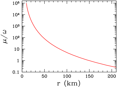
Figure 3: Neutrino-neutrino interaction strength $\mu$ in units of $\omega$ for our toy model of supernova neutrino oscillations.

Furthermore, we assume that (i) we have equal fluxes of neutrinos and antineutrinos, (ii) all of them are initially in the same flavour, (iii) the mass hierarchy is inverted, and (iv) the mixing angle is $\sin 2\tilde{\theta}_{0}=0.001$, representing a possibly small $\Theta_{13}$ mixing angle. We then find numerically the survival probability of the initial flavour as shown in Fig. 4.

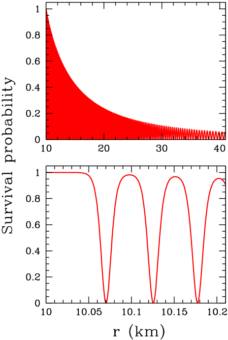
Figure 4: Survival probabilities for $\nu_{e}$ or $\bar{\nu}_{e}$ in our toy supernova model with symmetric initial conditions.

As expected, we observe in Fig. 4 bipolar oscillations above the neutrino sphere at $r=10$ km. Moreover, we observe that the oscillation amplitude declines as a function of radius so that after a few tens of km we obtain complete flavour conversion. The question then is: can the decline of the upper envelope of the survival probability be explained by way of the flavour pendulum?

In the pendulum language, we start at small radii with the usual full oscillations. However, while the pendulum oscillates, we slowly reduce $\mu$, i.e., we increase adiabatically the moment of inertia $I=\mu^{-1}$. Since the kinetic energy is $D^{2}/2I$ and the angular momentum $D$ is conserved, an increase in $I$ corresponds to a decrease in the kinetic energy. This is akin to a dancer who can speed up or slow down a pirouette by changing the moment of inertia. The continuous decrease in $\mu$ and hence in the kinetic energy, however, means that during subsequent swings, the pendulum will be unable to reach its previous height. This explains the general feature of a declining upper envelope in the survival probability caused by a decreasing $\mu$ (Fig. 4).

It is important to note that the potential energy is independent of $\mu$; it depends only on $\omega$. Therefore, our pendulum is not like a gravitational one where the potential energy would be affected by a changing mass. Instead, we can imagine the bob of the pendulum being charged and feeling the force of a homogeneous electric field.

Let us now quantify the decline of the upper envelope in Fig. 4. The kinetic energy at a given time is $T=\mu(t)D(t)^{2}/2$. The conservation of angular momentum, except for the natural pendulum motion, implies that a sudden change $\Delta\mu$ at some time $t$ causes a change in kinetic energy of $\Delta T=\Delta\mu D(t)^{2}/2$. For example, if we change $\mu$ by $\Delta\mu$ when the pendulum swings past its lowest point at which the kinetic energy is maximal, then the relative change is $\Delta T_{\rm max}/T_{\rm max}=\Delta\mu/\mu$. However, $\mu$ decreases slowly compared to the oscillation period so that we may assume a linear decline. Therefore, the change of $T_{\rm max}$ occurs over the entire oscillation period and thus must be weighted with a factor proportional to $D(t)^{2}$ over one oscillation period. If the oscillation is approximately harmonic, we have $D(t)^{2}\propto\sin^{2}(\kappa t)$ with $\kappa$ the pendulum’s natural frequency. The average of $\sin^{2}(\kappa t)$ is $1/2$. Therefore, if over one period $\mu$ decreases by a factor $(1-\epsilon)$ where $\epsilon\ll 1$, then $\Delta T_{\rm max}/T_{\rm max}=-\epsilon/2$. In other words, $T_{\rm max}$ is reduced by a factor $(1-\epsilon/2)=(1-\epsilon)^{1/2}$ so that $T_{\rm max}\propto\mu^{1/2}$.

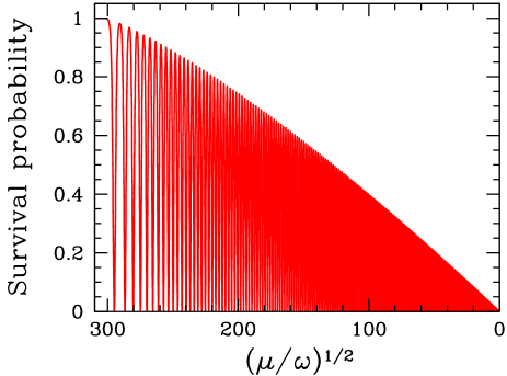
Figure 5: Survival probability for $\nu_{e}$ or $\bar{\nu}_{e}$ as in Fig. 4, here plotted as a function of $(\mu/\omega)^{1/2}$.

The maximal kinetic energy equals the maximal potential energy minus its minimum, achieved within one oscillation. The potential energy normalised such that its minimum is zero, $\omega\left(2+{\bf B}\cdot{\bf Q}\right)$ for small mixing angles and for large $\mu/\omega$, gives us the projection of the summed polarisation vector ${\bf S}$ on the flavour axis. Therefore, the upper envelope of the survival probability in Fig. 4 should scale with $\mu^{1/2}$. In Fig. 5 we show the same survival probabilities with $(\mu/\omega)^{1/2}$ as a radial coordinate. The decline is indeed nearly linear, especially for small-amplitude oscillations (toward the right side of the plot) where the pendulum oscillations are more nearly harmonic.

Our pendulum analogy elegantly explains the most puzzling feature of the bipolar supernova neutrino oscillations, i.e., that they actually lead to flavour conversion rather than permanent bipolar oscillations. We are simply seeing the relaxation of the pendulum to its downward rest position as kinetic energy is extracted by the reduction of the neutrino-neutrino interaction potential and thus the increase of the pendulum’s inertia.

V Neutrino Asymmetry

V.1 Realistic supernova example

The behaviour of neutrinos streaming off a supernova core looks, however, rather different from this simple picture. Besides the dependence of $\mu$ on the radius, another crucial feature is the initial neutrino-antineutrino asymmetry; the number flux of $\nu_{e}$ is the largest, that of $\bar{\nu}_{e}$ smaller, and those of the other species yet smaller but equal to one another. We represent this situation by the initial conditions $P_{z}(0)=1$ and $\bar{P}_{z}(0)=0.8$. The equations of motion for this system are simply those given in Sec. II.1. Solving them numerically yields the relative $\nu_{e}$ and $\bar{\nu}_{e}$ fluxes shown in Fig. 6. Plotting relative fluxes instead of survival probabilities makes conservation of the net flavour-lepton flux evident.

Observe that the initial flavour-lepton asymmetry is conserved so that there remains a net flux of $\nu_{e}$ originally set at $r=10$ km. Otherwise there is complete flavour conversion over a length scale given by the decrease of $\mu$ as a function of radius. Similar results are found in detailed numerical studies within the “one-angle approximation” where the neutrino interaction strength is taken equal for all modes (Fig. 8c of Ref. Duan:2006an and private communication by S. Pastor and R. Tomàs based on the numerical scheme of Ref. Pastor:2002we ). Changing the vacuum mixing angle and adding normal matter causes only the minor logarithmic changes predicted earlier.

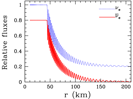
Figure 6: Relative fluxes of $\nu_{e}$ (blue/dotted) and $\bar{\nu}_{e}$ (red/solid) in our toy supernova model with 20% fewer antineutrinos than neutrinos and $\sin 2\tilde{\theta}_{0}=0.001$.

The behaviour of the neutrino ensemble between the neutrino sphere at 10 km and $r\approx 45$ km is explained by synchronised oscillations due to the neutrino-antineutrino asymmetry and the large value of $\mu$ in this region. Beyond this we enter the bipolar regime out to about 200 km when vacuum oscillations take over. In other words, the flavour evolution of neutrinos streaming off a supernova core are determined by a transition from synchronised oscillations at small radii (large $\mu$), bipolar oscillations at intermediate radii (intermediate $\mu$), and ordinary vacuum oscillations at large radii (small $\mu$) as first stressed in Ref. Duan:2005cp . If ordinary matter is included, it affects the synchronised region at small radii in the usual way by making the effective mixing angle smaller, and likewise at large radii where no collective effects occur. It is only in the intermediate, bipolar oscillation regime where ordinary matter has no significant impact on the system. Confusingly, the bipolar behaviour does not correspond to the limit of large or small neutrino densities; it corresponds to intermediate densities Duan:2005cp .

We have already explained the decline of the upper envelope of these curves in the bipolar regime which should scale as $\mu^{1/2}$. To confirm this behaviour once more we show in Fig. 7 (middle panel) the relative fluxes of Fig. 6 with $(\mu/\omega)^{1/2}$ as a radial coordinate. The decline of both the upper and lower envelopes are stunningly linear. This reflects the small-amplitude nature of the oscillations which are now nearly harmonic so that our previous argument works better here than in the previous section.

V.2 Transition between different oscillation modes

The lepton asymmetry of the neutrino flux is crucial for understanding a realistic supernova case. To develop a first understanding of this situation we consider an asymmetric ensemble with the initial condition $\bar{\bf P}(0)=\alpha{\bf P}(0)$ where $0\leq\alpha\leq 1$. If the $\nu$-$\nu$ interaction is sufficiently strong, the two polarisation vectors will hang together by their “internal magnetic field” and all vectors ${\bf P}$, $\bar{\bf P}$, ${\bf S}$, and ${\bf D}$ precess around ${\bf B}$ with the same synchronised frequency. Using $\dot{\bf D}=\omega{\bf B}\times{\bf S}$ and ${\bf D}={\bf S}(1-\alpha)/(1+\alpha)$, we thus find the usual result

$$\omega_{\rm synch}=\frac{1+\alpha}{1-\alpha}\,\omega\,.$$ (32)

Observe that the synchronised motion is faster for more symmetric systems!

To achieve synchronised oscillations, the internal frequencies of the system, i.e., their precession frequency around a common spin, must exceed the slow precession around the external magnetic field $\omega_{\rm synch}$. In our case of two polarisation vectors, the internal motion is described by $\dot{\bf S}=\mu{\bf D}\times{\bf S}$. When synchronisation prevails, ${\bf D}$ has a fixed length $(1-\alpha)$ so that the internal frequency is $(1-\alpha)\,\mu$. Successful synchronisation means that this frequency must exceed $\omega_{\rm synch}$, or, equivalently,

$$\frac{1+\alpha}{1-\alpha}\,\omega\lesssim(1-\alpha)\,\mu\,.$$ (33)

This is exactly the argument and result presented in Ref. Duan:2005cp . When this condition is violated, the motion becomes bipolar.

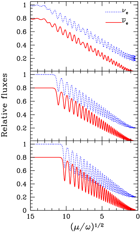
Figure 7: Relative fluxes of $\nu_{e}$ (blue/dotted) and $\bar{\nu}_{e}$ (red/solid) as in Fig. 6, here using $(\mu/\omega)^{1/2}$ as a radial coordinate. Top: Vacuum mixing angle $\sin 2\tilde{\theta}_{0}=0.1$. Middle: $\sin 2\tilde{\theta}_{0}=10^{-3}$ as in Fig. 6. Bottom: $\sin 2\tilde{\theta}_{0}=10^{-5}$.

Actually, this condition derives from an even simpler argument if we consider the total energy of the system,

$$H=\omega{\bf B}\cdot({\bf P}+\bar{\bf P})+\frac{\mu}{2}\,({\bf P}-\bar{\bf P})^{2}\,.$$ (34)

Synchronised oscillations require that the energy of the system be dominated by the spin-spin interaction, the second term. Assuming a small vacuum mixing angle so that ${\bf B}$ is nearly aligned with the initial polarisation vectors, and observing that $|{\bf P}+\bar{\bf P}|=1+\alpha$ and $|{\bf P}-\bar{\bf P}|=1-\alpha$, the requirement that the spin-spin term dominates is $\omega\,(1+\alpha)\lesssim(1-\alpha)^{2}\,\mu/2$, identical with Eq. (33) up to a multiplicative factor.

In other words, synchronised oscillations occur when the neutrino-neutrino part of the Hamiltonian always dominates over the vacuum-oscillation part, even for the most disadvantageous orientation of the polarisation vectors. At the other extreme, no collective effects obtain when the neutrino-neutrino part never dominates, even for the most advantageous orientation of these vectors, i.e., when $\mu\lesssim\omega$. The bipolar regime corresponds to the intermediate range where the relative magnitude of the different energy contributions depends on the orientation of the polarisation vectors. In summary, bipolar oscillations are expected when

$$\omega\lesssim\mu<4\frac{(1+\alpha)}{(1-\alpha)^{2}}\,\omega,$$ (35)

and thus occur for an intermediate strength of the neutrino-neutrino interaction, i.e., an intermediate range of neutrino densities as first discussed in Ref. Duan:2005cp . The exact numerical factor on the r.h.s. of this equation is taken from Eq. (46) below.

V.3 Asymmetric system as a pendulum with spin

This simple reasoning gives us the correct scale for the transition between synchronised and bipolar oscillations, but does not explain the nature of the transition. The two oscillation modes must be extreme cases of a continuum, yet the nature of the intermediate cases is not obvious. It turns out that this continuum has a straightforward physical interpretation that is quite illuminating for an understanding of the entire system.

To this end we note that the asymmetric system is described by the same equations of motion (II.1) for ${\bf Q}$ and ${\bf D}$ as the symmetric case, and $Q=|{\bf Q}|$ is likewise conserved. The new feature here is the initial condition ${\bf D}(0)\not=0$ and ${\bf D}\cdot{\bf Q}\not=0$, so that Eq. (II.1) now implies

$${\bf D}=\frac{1}{\mu}\,\frac{{\bf Q}\times\dot{\bf Q}}{Q^{2}}+\frac{{\bf D}\cdot{\bf Q}}{Q^{2}}\,{\bf Q}\,.$$ (36)

Since

$$\sigma={\bf D}\cdot{\bf Q}/Q$$ (37)

is a constant of the motion, the expression (36) can be equivalently written as

$${\bf D}=\frac{{\bf q}\times\dot{\bf q}}{\mu}+\sigma\,{\bf q}\,,$$ (38)

with ${\bf q}={\bf Q}/Q$. The first term in the expression corresponds to the orbital angular momentum as before, while the second term plays the role of an inner angular momentum (i.e., spin) of the pendulum’s bob. This spin is always along the direction ${\bf q}$, implying that we should think of the system as a spinning top mounted in a way that its axis of rotation can swing like a pendulum. If the top has no spin (i.e., $\sigma=0$), it acts as an ordinary spherical pendulum.

Starting with the equation of motion $\dot{\bf D}=\omega{\bf B}\times{\bf Q}$ and observing that $\dot{\bf q}\times\dot{\bf q}=0$, we find

$$\frac{{\bf q}\times\ddot{\bf q}}{\mu}+\sigma\,\dot{\bf q}=\omega Q{\bf B}\times{\bf q}\,.$$ (39)

For the case $\sigma=0$, we recover the equation of motion of a pendulum swinging in the plane defined by ${\bf B}$ and the initial vector ${\bf q}(0)$ which we always choose to be in the $z$-direction. Conversely, if $\mu$ is so large that we can neglect the first term, we are back to a spin-precession equation with a precession frequency $\omega_{\rm precess}=\omega Q/\sigma$. For $\mu\gg\omega$ we have

$$Q \approx 1+\alpha\,,$$

$$\sigma \approx 1-\alpha\,,$$ (40)

so $\omega_{\rm precess}$ is indeed equal to $\omega_{\rm synch}$ of Eq. (32).

The extreme cases thus have an intuitive interpretation. Synchronised oscillations correspond to the flavour top spinning so fast that its response to the force field is precession, just like a spun-up top on a flat table surface. On the other hand, if the top spins slowly (corresponding to the case of a small neutrino asymmetry), then it swings like an ordinary pendulum; the inner angular momentum in this case has little impact, and we are in the bipolar mode.

Let us consider the asymmetric system in more detail. Several conserved quantities are apparent. One is the energy of the system,

$$E = E_{\rm pot}+E_{\rm kin}$$ (41)

$$= \omega Q\,({\bf B}\cdot{\bf q}+1)+\frac{\mu}{2}{\bf D}^{2}$$

$$= \omega Q\,({\bf B}\cdot{\bf q}+1)+\frac{1}{2\mu}\,\dot{\bf q}^{2}+\frac{\mu}{2}\,\sigma^{2}\,,$$

where we have added a constant to the potential energy such that it vanishes when the pendulum is oriented opposite to the force field. The other conserved quantity is the projection of ${\bf D}$ in the ${\bf B}$ direction, corresponding to the conservation of that component of the angular momentum parallel to the force field and which is thus not subject to a torque.

The conservation of angular momentum implies that the initial lepton asymmetry cannot be changed beyond the amount caused by ordinary vacuum oscillations. In all practical cases we begin with ${\bf D}$ oriented along the $z$-axis, while ${\bf B}$ is tilted by $2\theta_{0}$. If $\theta_{0}$ is small, the initial neutrino asymmetry is almost perfectly conserved. Thus the self-interacting system cannot stimulate an exotically large flavour conversion effect.

If the spin is not quite fast enough for perfect precession, the overall motion is a wobble. The spinning top starts in a nearly upright position, its axis pointing nearly to the north pole. It will tilt a bit until it reaches a certain latitude, when its motion reverses back to the north pole. The latitude of reversal will lie further south if either or both of $\sigma$ and $\mu$ is smaller. In other words, a smaller $\nu$-$\nu$ term makes the system “more bipolar”. A more symmetric system (smaller $\sigma$) is also more bipolar.

The southernmost position the pendulum can reach is defined by energy and angular momentum conservation. As an example, we take the mixing angle to be very small so that ${\bf B}$ is very close to the $z$-direction. In this approximation, the initial total energy is $E=2\omega Q+\mu\sigma^{2}/2$ and energy conservation implies

$$\omega Q(1-\cos\varphi)=\frac{\dot{\bf q}^{2}}{2\mu}\,.$$ (42)

On the other hand, angular momentum conservation along the ${\bf B}$-direction gives

$$\sigma=\sigma\cos\varphi+\mu^{-1}\dot{q}_{\perp}\sin\varphi\,,$$ (43)

where $\dot{q}_{\perp}$ is the velocity perpendicular to ${\bf B}$, i.e., the pendulum’s velocity along a circle of latitude. The largest excursion $\varphi_{\rm max}$ is reached when the pendulum reverses its motion at its southernmost position where $\dot{\bf q}^{2}=\dot{q}_{\perp}^{2}$. Combined with Eqs. (42) and (43), we find

$$\cos\varphi_{\rm max}=\frac{\mu\sigma^{2}}{2\omega Q}-1\,$$ (44)

for the largest excursion angle.

As expected, if either or both of $\mu$ and $\sigma$ becomes smaller, Eq. (44) tells us that the pendulum reaches more southern latitudes. On the other hand, the equation has no solution for

$$\mu\sigma^{2}>4\omega Q\,.$$ (45)

This condition corresponds to the fully synchronised case, which prohibits any deviation from perfect $z$-alignment because of our artificial assumption of ${\bf B}$ and the initial $\bf{P}$ and $\bar{\bf{P}}$ being exactly aligned. If the pendulum had not initially been perfectly aligned with ${\bf B}$, solutions would exist for all values of the parameters. Still, for small mixing angles, Eq. (45) provides an excellent estimate of the condition for synchronised behaviour. Using Eq. (V.3), this condition is equivalent, in the $\mu/\omega\gg 1$ limit, to

$$\frac{(1-\alpha)^{2}}{1+\alpha}>4\,\frac{\omega}{\mu},$$ (46)

where, we recall, $\alpha$ parameterises the lepton asymmetry by virtue of $|\bar{\bf P}|=\alpha|{\bf P}|$.

Taking our previous asymmetric example with $P_{z}(0)=1$ and $\bar{P}_{z}(0)=0.8$ (i.e., $\alpha=0.8$) and assuming $\mu\gg\omega$, synchronised behaviour is expected for $\mu/\omega>180$ or $(\mu/\omega)^{1/2}>13.4$. This estimate corresponds well with the onset of synchronisation in the top panel of Fig. 7 where the mixing angle is large. Of course, the true point of onset also depends logarithmically on the mixing angle—see the other panels of Fig. 7.

It is now evident that the onset of bipolar oscillations does not imply full conversions. As we move into the bipolar regime, the spinning top begins to wobble, reaching only some southern latitude, but not the south pole. How far south it will get, i.e., the spread between the upper and lower envelopes in Fig. 7, depends on the details of how the system enters the bipolar regime. If the mixing angle is large, bipolar oscillations begin almost immediately so that the amplitude of the oscillations will be small. If the mixing angle is small, the delayed onset of the first bipolar swing allows $\mu$ to decrease further, thereby resulting in a more southern turning point. Therefore, smaller mixing angles imply a later onset of oscillations and a larger spread between the envelopes. This is borne out by the examples shown in Fig. 7, where $\sin 2\tilde{\theta}_{0}=0.1$, $10^{-3}$ and $10^{-5}$ from top to bottom.

V.4 Equipartition of Energies

We have noted that the energy of the spinning top decreases in proportion to $\mu^{1/2}$ once it has entered the bipolar regime, assuming the decline of $\mu$ is sufficiently slow. It is illuminating to note that from that time onward, the total energy Eq. (41) is equipartitioned between $E_{\rm pot}$, the potential energy in the external force field, and $E_{\rm kin}$, the internal and orbital kinetic energy of the spinning top (equivalent to the neutrino-neutrino interaction energy).

Figure 8: Different energy components $E_{\rm pot}$, $E_{\rm kin}$ and $E_{\rm tot}/2$ for the schematic supernova model of Fig. 6, using $(\mu/\omega)^{1/2}$ as a radial coordinate. The panels from top to bottom have the vacuum mixing angle $\sin 2\tilde{\theta}_{0}=0.1$, $10^{-3}$ and $10^{-5}$, respectively. The vertical line at $\mu/\omega=\sqrt{180}\approx 13.4$ marks the transition to the bipolar regime according to Eq. (46) for this example where $\alpha=0.8$.

To illustrate this point we show for our toy supernova the evolution of $E_{\rm pot}$, $E_{\rm kin}$ and $E_{\rm tot}/2=(E_{\rm pot}+E_{\rm kin})/2$ in Fig. 8, using once more $(\mu/\omega)^{1/2}$ as a radial coordinate. Observe that indeed $E_{\rm pot}=E_{\rm kin}$ at $\mu/\omega=180$ or $(\mu/\omega)^{1/2}=13.4$ for our example $\alpha=0.8$. It is intriguing that the transition between the synchronised and the bipolar regime is practically independent of the mixing angle. The same is true also for the total energy $E_{\rm tot}$, which decreases very nearly as $\mu^{1/2}$ in the bipolar regime as explained earlier. In the synchronised regime close to the supernova, the potential energy does not depend on $\mu$ whereas the kinetic energy decreases with $\mu$. In the bipolar region, on the other hand, the kinetic and potential energies are nearly equipartitioned after averaging over the pendulum’s nutation period.

To understand this equipartition effect analytically, we consider a case where the nutation amplitude is very small as in the top panel of Fig. 8 (large mixing angle), so that it suffices to study only the precession, i.e., we assume the pendulum’s orbital motion is such that its velocity is along a circle of latitude. As a function of excursion angle $\varphi$, the total energy is

$$E_{\rm tot}=\omega Q(1+\cos\varphi)+\frac{\dot{\bf q}^{2}}{2\mu}+\frac{\mu}{2}\sigma^{2}\,.$$ (47)

Using angular-momentum conservation Eq. (43) and the relation $\dot{\bf q}^{2}=\dot{q}_{\perp}^{2}$ to eliminate the orbital velocity, we find

$$E_{\rm tot}=\omega Q(1+\cos\varphi)+\frac{\mu\sigma^{2}}{2}\,\frac{1}{1+\cos\varphi}\,.$$ (48)

We further recall that the system enters the bipolar regime when $\mu\sigma^{2}=4\omega Q$, and that at this point the excursion angle is still small so that $\cos\varphi=1$. Therefore, $E_{\rm pot}=E_{\rm kin}=2\omega Q$ at the onset of the bipolar regime. Subsequently, $E_{\rm tot}$ is expected to scale as $\mu^{1/2}$ so that $E_{\rm tot}=(4\omega Q\mu\sigma^{2})^{1/2}$. We can now solve for the expression $(1+\cos\varphi)$ as a function of $\mu$ and find explicitly $E_{\rm pot}=E_{\rm kin}=(\omega Q\mu\sigma^{2})^{1/2}$.

An important detail is that equipartition cannot hold all the way to very small $\mu$. Angular momentum conservation, i.e., the approximate conservation of the net $\nu_{e}$ flux in the limit of a small vacuum mixing angle, implies that the potential energy is bounded from below. In terms of polarisation vectors, this means that the strict conservation of ${\bf B}\cdot{(\bf P}-\bar{\bf P})$ leads to an approximately constant $P_{z}-\bar{P}_{z}=1-\alpha=\sigma$ in the case of small vacuum mixing. Therefore, the smallest allowed value of the potential energy is

$$E_{\rm pot}\geq 2(1-\alpha)\omega=2\sigma\omega\,.$$ (49)

In the example of Fig. 8 we have used an asymmetry $\alpha=0.8$. This gives an analytic estimate of $E_{\rm pot}\geq 0.4\,\omega$ using Eq. (49), which is in excellent agreement with numerical results. On the other hand, the kinetic energy, being proportional to $\mu$, must eventually vanish. Therefore, $E_{\rm pot}$ and $E_{\rm kin}$ approach different limits as $\mu\to 0$, as borne out by Fig. 8.

Therefore, the evolution of the system now appears in a different light. When $\mu$ decreases slowly, the system never properly enters the bipolar regime: it stays at the edge of it. The polarisation vectors spiral and slowly tilt in such a way that their energy in the external $B$-field and the internal spin-spin energies stay equal to the degree allowed by net lepton number conservation.

VI Many Modes

VI.1 Multiple frequencies

We now turn to a more realistic case of an ensemble of $\nu_{e}$ and $\bar{\nu}_{e}$ with different energies, i.e., different vacuum oscillation frequencies $\omega_{i}$. The equations of motion are

$$\partial_{t}{\bf P}_{i} = \left[+\omega_{i}{\bf B}+\mu\left({\bf P}-\bar{\bf P}\right)\right]\times{\bf P}_{i}\,,$$

$$\partial_{t}\bar{\bf P}_{i} = \left[-\omega_{i}{\bf B}+\mu\left({\bf P}-\bar{\bf P}\right)\right]\times\bar{\bf P}_{i}\,,$$ (50)

where for $N$ modes we use

$${\bf P}=\sum_{i=1}^{N}{\bf P}_{i}\hbox{\qquad and\qquad}\bar{\bf P}=\sum_{i=1}^{N}\bar{\bf P}_{i}\,.$$ (51)

We keep the normalisation $|{\bf P}|=|\bar{\bf P}|=1$ for the entire ensemble so that the individual modes are normalised to $|{\bf P}_{i}|=|\bar{\bf P}_{i}|=N^{-1}$.

In full analogy to the previous treatment we introduce the vectors ${\bf S}_{i}={\bf P}_{i}+\bar{\bf P}_{i}$ and ${\bf D}_{i}={\bf P}_{i}-\bar{\bf P}_{i}$ as well as ${\bf D}=\sum{\bf D}_{i}={\bf P}-\bar{\bf P}$ so that

$$\dot{\bf S}_{i} = \omega_{i}{\bf B}\times{\bf D}_{i}+\mu{\bf D}\times{\bf S}_{i}\,,$$

$$\dot{\bf D}_{i} = \omega_{i}{\bf B}\times{\bf S}_{i}+\mu{\bf D}\times{\bf D}_{i}\,.$$ (52)

Each pair of modes ${\bf P}_{i}$ and $\bar{\bf P}_{i}$ evolves symmetrically so that each ${\bf D}_{i}$ is always oriented along the $y$-axis and the terms ${\bf D}\times{\bf D}_{i}$ vanish.

We now assume strong coupling with $\mu/\omega_{i}\gg 1$ for all modes so that we can also drop the $\omega_{i}{\bf B}\times{\bf D}_{i}$ term. This leaves us with the approximate equations of motion

$$\dot{\bf S}_{i} = \mu{\bf D}\times{\bf S}_{i}\,,$$

$$\dot{\bf D}_{i} = \omega_{i}{\bf B}\times{\bf S}_{i}\,.$$ (53)

Equation (VI.1) implies that all ${\bf S}_{i}$ evolve in the same way because they precess in the same field ${\bf D}$. Flavour conversion is now described by a single vector ${\bf S}=\sum{\bf S}_{i}$ (and thus ${\bf S}_{i}={\bf S}/N$), and governed by

$$\dot{\bf S} = \mu{\bf D}\times{\bf S}\,,$$

$$\dot{\bf D} = \left(\frac{1}{N}\sum_{i}^{N}\omega_{i}\right){\bf B}\times{\bf S}\,.$$ (54)

Thus, the evolution of the flavour content proceeds in the same way as before [cf. Eq. (II.1)], but with the role of $\omega$ replaced with the average oscillation frequency of all modes $\langle\omega\rangle\equiv N^{-1}\sum_{i}^{N}\omega_{i}$.

On the level of the individual modes, the “tilting motion” around the $y$-axis is the same for all neutrino and antineutrino modes, so in this sense their motion is synchronised. On the other hand, the transverse motion characterised by ${\bf D}_{i}$ is different for every mode because before summing, the equations of motion are

$$\dot{\bf S} = \mu{\bf D}\times{\bf S}\,,$$

$$\dot{\bf D}_{i} = \omega_{i}\frac{{\bf B}\times{\bf S}}{N}\,,$$ (55)

where we have used ${\bf S}_{i}={\bf S}/N$.

It is, therefore, incorrect to say that all modes form two block spins ${\bf P}$ and $\bar{\bf P}$ which evolve separately in the bipolar sense, with each individual mode staying aligned with its respective block spin. Separate alignment for neutrinos and antineutrinos was explicitly claimed, for example, above Eq. (4.1) in Ref. Kostelecky:1995dt , in reference to the authors’ own numerical studies of Refs. Kostelecky:1993dm ; Kostelecky:1994ys . However, the observation of separate alignment does not appear to be documented or demonstrated in these papers. Whatever the origin of these authors’ observation of bipolar alignment, it is in conflict with our analytic treatment. We have numerically verified that bipolar alignment does not hold and that our individual ${\bf P}_{i}$ and $\bar{\bf P}_{i}$ vectors do indeed evolve differently, as shown in Fig. 9.

The $z$-components of all modes evolve identically while the transverse motion is different for modes with different $\omega_{i}$. The transverse motion for the neutrino and antineutrino polarisation vectors are opposite so that neutrinos and antineutrinos form two distinct cohorts. In this sense the evolution actually is bipolar. Therefore, we stick to this established terminology, keeping in mind a broad interpretation of the word “bipolar.”

The most important conclusion is that the strongly interacting multi-mode system is exactly equivalent to one mode if one interprets the vacuum oscillation frequency $\omega$ as the average of all modes. Therefore, the entire system is still characterised by a single collective variable. This conclusion also holds for the asymmetric system of unequal densities of $\nu$ and $\bar{\nu}$. The variation of different vacuum oscillation frequencies is not a source of kinematical decoherences and the system behaves, in this sense, similarly to synchronised oscillations.

Figure 9: Evolution of the individual modes $P_{y}$ (red/solid) and $\bar{P}_{y}$ (blue/dotted) in a 4-mode system described by Eq. (VI.1), with $\tilde{\theta}_{0}=0.01$ (i.e., inverted hierarchy), $\omega_{i}=1,2,3,4$ for $i=1$, 2, 3, and 4, respectively, and strong neutrino-neutrino interaction $\mu=100$.

VI.2 Different interaction strengths

Instead of different frequencies one may also consider different coupling constants between different modes. In this case, the general equations of motion are

$$\partial_{t}{\bf P}_{i} = \left[+\omega_{i}{\bf B}+\sum_{j=1}^{N}\mu_{ij}\left({\bf P}_{j}-\bar{\bf P}_{j}\right)\right]\times{\bf P}_{i}\,,$$

$$\partial_{t}\bar{\bf P}_{i} = \left[-\omega_{i}{\bf B}+\sum_{j=1}^{N}\mu_{ij}\left({\bf P}_{j}-\bar{\bf P}_{j}\right)\right]\times\bar{\bf P}_{i}\,.$$ (56)

Variations in the interaction coefficients are motivated by their dependence on the relative angle of the neutrino trajectories. Neutrinos streaming off a supernova core are far from isotropic so that unequal $\mu_{ij}$ coefficients are unavoidable. The recent multi-angle simulations were aiming precisely at this issue Duan:2006an ; Duan:2006jv .

Even in an isotropic medium the coupling constants between the different modes are never equal, but involve a factor $(1-\cos\theta_{\bf pq})$ from the current-current structure of the weak-interaction Hamiltonian. However, isotropy implies that all modes with different momenta ${\bf p}$ but identical $p=|{\bf p}|$ evolve in the same way. Therefore, the angular part of the integral in Eq. (A.1) can be trivially performed in the sense that the $\cos\theta_{\bf pq}$ term averages to zero. The isotropic system is thus equivalent to the case of multiple frequencies, but a common coupling constant described in Sec. VI.1. In other words it is equivalent to the “single-angle” case.

In terms of our variables ${\bf S}_{i}$ (the flavour-dependent particle plus antiparticle number) and ${\bf D}_{i}$ (the net lepton number), the equations of motion are

$$\dot{\bf S}_{i} = \omega_{i}{\bf B}\times{\bf D}_{i}+\sum_{j=1}^{N}\mu_{ij}{\bf D}_{j}\times{\bf S}_{i}\,,$$

$$\dot{\bf D}_{i} = \omega_{i}{\bf B}\times{\bf S}_{i}+\sum_{j=1}^{N}\mu_{ij}{\bf D}_{j}\times{\bf D}_{i}\,.$$ (57)

For the global ${\bf S}$ and ${\bf D}$ vectors this implies

$$\dot{\bf S} = \sum_{i=1}^{N}\omega_{i}{\bf B}\times{\bf D}_{i}+\sum_{i,j=1}^{N}\mu_{ij}{\bf D}_{j}\times{\bf S}_{i}\,,$$

$$\dot{\bf D} = \sum_{i=1}^{N}\omega_{i}{\bf B}\times{\bf S}_{i}\,,$$ (58)

where we have used the symmetry $\mu_{ij}=\mu_{ji}$. Equation (VI.2) cannot be brought into the form of a closed set of equations. However, even in this general case the quantity ${\bf B}\cdot{\bf D}$ is a constant of the motion. This means that bipolar oscillations never lead to lepton number conversions beyond the amount caused by vacuum mixing.

It is possible to formulate a sufficient condition for a multiple-coupling constant system to behave as a simple flavour pendulum. Starting with Eq. (VI.2) we note that the system acts as a single flavour pendulum if all ${\bf S}_{i}$ and ${\bf D}_{i}$ tilt with the same speed. Self-consistency then requires that all frequencies are equal, $\omega_{i}\equiv\omega$, and that

$$\sum_{j=1}^{N}\mu_{ij}=\mu\,,$$ (59)

with $\mu$ a number that is independent of $i$. In addition, symmetry between different modes requires that $\mu_{ij}=\mu_{ji}$. These conditions are met, for example, if

$$\mu_{ij}\propto g\left(\frac{i-j}{N}\right)\,,$$ (60)

where $g(x)$ is an even function that is periodic in the sense $g(x+1)=g(x)$. An example is $g(x)=\cos(2\pi x)$.

An important case where these conditions are violated is neutrinos radiated from a supernova core. Assuming overall spherical symmetry, the only parameter that differentiates between trajectories is $\cos\theta$ with $\theta$ the angle relative to the radial direction. Considering instead the schematic case of neutrinos emitted “isotropically” by a plane surface, the coupling constants are Duan:2006an , following Eq. (78),

$$\mu_{ij} = \mu\,\frac{4}{3}\,(1-c_{i}c_{j})$$ (61)

$$= \mu\,\frac{4}{3}\,\left[1-\frac{(i-\frac{1}{2})(j-\frac{1}{2})}{N^{2}}\right]\,.$$

Here, $c_{i}=\cos\theta_{i}$ is the cosine of the neutrino mode relative to the radiating surface’s normal direction. We assume a uniform distribution in $0\leq c_{i}\leq 1$ represented by discrete modes as in the second line of Eq. (61). Note that $\sum_{i=1}^{N}(i-\frac{1}{2})=N^{2}/2$ so that the average $\langle\mu_{ij}\rangle=\mu$ is exact, even for a small number of modes.

This example does not satisfy the condition Eq. (59) because

$$\sum_{j=1}^{N}\mu_{ij}=\mu\,\frac{4N}{3}\left[1-\frac{i-\frac{1}{2}}{2N}\right]\,.$$ (62)

(Note that the overall factor of $N$ is compensated by using individual polarisation vectors that are normalised to the length $N^{-1}$.) Therefore, one cannot expect neutrinos streaming off a supernova core to oscillate in a collective manner. Rather, one should expect kinematical decoherence within a few bipolar periods, i.e., on a time scale of order $\kappa^{-1}=(\omega\mu)^{1/2}$. In other words, the length of the total ${\bf P}$ or $\bar{\bf P}$ vector is no longer conserved and the ensemble partly or fully decoheres.

In simple numerical examples of a symmetric system this expectation is indeed borne out, i.e., a non-isotropic ensemble consisting of equal numbers of neutrinos and antineutrinos turns into an equal mixture of both flavours within a few bipolar oscillation periods for both the normal and inverted hierarchy.

On the other hand, the large-scale numerical studies of Ref. Duan:2006an show that neutrinos streaming off a supernova core are sometimes quite well represented by the single-angle case, i.e., collective behaviour rather than quick kinematical decoherence appears to be more generic. Again, the main differences to a simple symmetric system are twofold: there is a neutrino-antineutrino asymmetry and the effective density declines with radius. We have already observed in Sec. V.4 that for the inverted hierarchy the asymmetry, together with the slow decline of the neutrino density, has the effect of slowly turning the polarisation vectors without the system ever entering the bipolar regime, i.e., the system teeters along the edge of the bipolar condition. Since the bipolar regime is never properly entered, it is less surprising that kinematical decoherence is not a prominent feature of the evolution.

A dedicated research project is required to develop a deeper understanding of the conditions that determine if the system evolves as as single collective system in the form of the flavour pendulum, or if it kinematically decoheres in that the individual polarisation vectors of the different modes are “randomised” in flavour space.

Our main conclusion is that different oscillation frequencies are not a source of kinematical decoherence, while the multi-angle nature of a non-isotropic system is such a source, especially for a symmetric system. The detailed interplay between the collective mode represented by our pendulum and the multi-modal nature of the non-isotropic system remains to be understood.

VII Connection to quantum physics

VII.1 Quantisation of the flavour pendulum

We have seen that the flavour conversion of neutrinos streaming off a supernova core can be understood almost completely when we cast the equations of motion in the form of a pendulum in flavour space that may include inner angular momentum if we need to account for a lepton asymmetry. One may then ask if flavour conversion was possible in the absence of flavour mixing since, even if the pendulum were placed exactly on its tip, Heisenberg’s uncertainty relation would prevent it from staying there forever, just as an idealised pencil cannot stand on its tip indefinitely.

To estimate the relevant time scale we recall that the equations of motion for the pendulum’s excursion angle can be derived from the classical Hamiltonian Eq. (14) with $\varphi$ and $D$ as the canonical variables. In order to quantise this system, however, we need to be more careful about absolute scales, and the equations of motion for the quantum variables must follow from the Hamiltonian of the full quantum system. In the case of $N$ neutrinos and $N$ antineutrinos, the full Hamiltonian is simply $N$ times the one of Eq. (14),

$$H_{\rm tot}=\frac{N}{2}\,\mu\,D^{2}+\frac{N\kappa^{2}}{\mu}\bigl{[}1-\cos(\varphi+2\theta_{0})\bigr{]}\,.$$ (63)

Identifying $\varphi$ as the canonical coordinate, the familiar equations of motion (II.3) follow classically using Hamilton’s equations, provided we interpret $ND$ as the conjugate momentum. The pendulum’s potential energy in the macroscopic sense scales with $N$, and likewise its moment of inertia $I=N/\mu$. On the quantum level, the corresponding commutation relation is

$$[\varphi,D]=\frac{{\rm i}\hbar}{N}\,.$$ (64)

Using this commutation relation, the same equations of motion (II.3) follow quantum mechanically from the full Hamiltonian (63) by way of Heisenberg’s equations of motion ${\rm i}\hbar\dot{\varphi}=[\varphi,H_{\rm tot}]$ and ${\rm i}\hbar\dot{D}=[D,H_{\rm tot}]$.

The fact that the same equations of motion for the tilt angle $\varphi$ follow both classically and quantum mechanically irrespective of the size of $N$—provided we identify the appropriate canonical momentum—indicates that the flavour evolution does not depend on the size of the system. Thus, as long as our calculation is classical, we can work with polarisation vectors and associated angular momenta that are normalised to unity. On the quantum level, however, the absolute length of the polarisation vectors will affect the quantisation of the system, and it is necessary that we use the correct Hamiltonian with the appropriate factors of $N$.

To estimate the time scale for the pendulum to stay upright we consider its downward vertical position, i.e., we consider it to be a harmonic oscillator in its quantum-mechanical ground state. The uncertainties of the canonical variables in this state are

$$\langle\varphi^{2}\rangle=\frac{1}{2}\,\frac{1}{I\kappa}\,,\quad\hbox{and}\quad\langle(ND)^{2}\rangle=\frac{1}{2}\,I\kappa\,,$$ (65)

where $\kappa$ is the oscillation frequency of the pendulum and $I=N/\mu$ its moment of inertia. In the strong-interaction limit $\mu\gg\omega$, the expression for $\langle\varphi^{2}\rangle$ becomes

$$\langle\varphi^{2}\rangle=\frac{1}{2N}\,\left(\frac{\mu}{2\omega}\right)^{1/2}\,.$$ (66)

Let us now put in some realistic numbers. The typical density of neutrinos in the supernova region of interest is estimated to be $10^{32}~{}{\rm cm}^{-3}$ in Appendix A before Eq. (77). The volume of the critical region may be of order $100~{}{\rm km}^{3}$ so that some $10^{53}$ particles may be in the system at any one time. Moreover, the bipolar regime begins at $(\mu/\omega)^{1/2}$ of order 10. Thus a typical value for $\langle\varphi^{2}\rangle^{1/2}$ would be of order $10^{-26}$. If this number is taken to be a typical excursion angle caused by quantum fluctuations, then the time scale to tilt will be of order $\kappa^{-1}\ln(10^{26})\approx 60\ \kappa^{-1}$. Since $\kappa^{-1}$ is a fraction of a km, the quantum effect would happen over a length scale of tens of km. Of course, the vacuum mixing angle and thus the initial excursion of the pendulum is much larger than this quantum estimate. Moreover, the system would be subject to other forces. Still, this estimate demonstrates that in an unstable system exponential growth can quickly enhance quantum effects to a macroscopic scale.

VII.2 Full quantum system

The discussion above shows that our classical treatment of the flavour evolution of a large neutrino ensemble was justified. However, it is still instructive to briefly explain the structure of the full quantum Hamiltonian. It is well known that the neutrino interaction in flavour space has an $SU(2)$ structure and as such is equivalent to a spin system Friedland:2003eh ; Friedland:2006ke ; Balantekin:2006tg . The equations of motion with a matter term (III) can be shown to follow from the quantum Hamiltonian

$$\hat{H} = \hat{H}_{0}+\hat{H}_{\rm matter}+\hat{H}_{\nu\nu}$$

$$= \omega{\bf B}\cdot(\hat{\bf S}-\hat{\bar{\bf S}})+\lambda{\bf L}\cdot(\hat{\bf S}+\hat{\bar{\bf S}})+\frac{\mu}{N}(\hat{\bf S}+\hat{\bar{\bf S}})^{2}\,,$$

where we now use carets to denote quantum operators explicitly. The operators $\hat{\bf S}$ and $\hat{\bar{\bf S}}$ each represent an angular momentum $N/2$, i.e., $N$ spin $\frac{1}{2}$ particles that are linked to form one big “block spin” each. The equation of motion for $\hat{\bf S}$ follows from ${\rm i}\hbar\partial_{t}\hat{\bf S}=[\hat{\bf S},\hat{H}]$ and the angular momentum commutation relation $[\hat{S}_{i},\hat{S}_{j}]={\rm i}\hbar\epsilon_{ijk}\hat{S}_{k}$ and similarly for $\hat{\bar{\bf S}}$. Note that $\hbar$ drops out of the spin-precession equation $\partial_{t}\hat{\bf S}=\omega{\bf B}\times\hat{\bf S}$. Therefore, spin precession is fundamentally a classical phenomenon and one does not need to distinguish carefully between equations of motion for quantum operators and for expectation values. However, for the nonlinear neutrino-neutrino term, it is not intuitively obvious that one can ignore correlation effects when taking the expectation values Friedland:2003dv ; Bell:2003mg .

The connection to the polarisation vectors is that ${\bf P}=\langle\hat{\bf S}\rangle\,(2/N)$ is the normalised expectation value of the spin that represents the particles, whereas $\bar{\bf P}=-\langle\hat{\bar{\bf S}}\rangle\,(2/N)$ includes a minus sign. In other words, the quantities ${\bf P}$ and $\bar{\bf P}$ play the role of “magnetic moments” in flavour space, whereas the quantities $\hat{\bf S}$ and $\hat{\bar{\bf S}}$ play the role of angular momenta. We call them “flavour spins,” but the terminology “neutrino flavour isospins (NFIS)” has also been used Duan:2005cp ; Duan:2006an ; Duan:2006jv . The negative sign between the polarisation vector and flavour spin for antineutrinos is consistent with antiparticles of equal spin carrying negative magnetic moments relative to the particles, such as the case of electrons and positrons. This negative sign also explains that under the mass Hamiltonian in vacuum $\hat{H}_{0}$, neutrinos and antineutrinos precess “in opposite directions” in flavour space. We find that the language of polarisation vectors is useful in the classical limit, whereas the language of flavour spins is useful when dealing with the quantum aspects of the system.

We note that only the vacuum Hamiltonian $\hat{H}_{0}$ distinguishes between neutrinos and antineutrinos, while the matter and $\nu$-$\nu$ parts of the full Hamiltonian can be expressed in terms of a single big angular momentum operator $\hat{\bf J}=\hat{\bf S}+\hat{\bar{\bf S}}$. Therefore, these parts of the Hamiltonian are equivalent for our system consisting of neutrinos and antineutrinos, and a neutrino-only system consisting of two flavours. In the neutrino-only case, “flavour spin up” means $\nu_{e}$, “flavour spin down” $\nu_{\mu}$. In our case, “flavour spin up” means either $\nu_{e}$ or $\bar{\nu}_{\mu}$, and “flavour spin down” $\bar{\nu}_{e}$ or $\nu_{\mu}$, and the states $\nu_{e}$ and $\bar{\nu}_{\mu}$ are fully equivalent in the absence of $\hat{H}_{0}$ (and similarly for $\bar{\nu}_{e}$ and $\nu_{\mu}$).

In terms of the big angular momentum operator $\hat{\bf J}$, we see that the neutrino-neutrino Hamiltonian is of the form $\hat{\bf J}^{2}$, while the interaction with ordinary matter is proportional to $\hat{J}_{z}$. These two operators commute so that they have a common set of energy eigenstates. This observation is the quantum analogue to our classical result that the presence of ordinary matter leaves bipolar oscillations nearly unaffected.

Some time ago it was speculated that a system of many spins interacting by a nonlinear Hamiltonian of the form $\hat{\bf J}^{2}$ could exhibit quantum entanglement effects in the sense that its evolution is coherently accelerated Bell:2003mg . Applied to our case, this conjecture means the following. Consider a “dense gas” consisting of exactly one $\nu_{e}$ and one $\bar{\nu}_{e}$ with the same density as our macroscopic system, i.e., with the same spin-spin interaction energy $\mu$. In this case the four possible states of the system are grouped into a triplet state consisting of $\left|\nu_{e},\bar{\nu}_{\mu}\right\rangle$, $\frac{1}{\sqrt{2}}(\left|\nu_{e},\bar{\nu}_{e}\right\rangle+\left|\nu_{\mu},\bar{\nu}_{\mu}\right\rangle)$ and $\left|\nu_{\mu},\bar{\nu}_{e}\right\rangle$, and a singlet state $\frac{1}{\sqrt{2}}(\left|\nu_{e},\bar{\nu}_{e}\right\rangle-\left|\nu_{\mu},\bar{\nu}_{\mu}\right\rangle)$. Put another way, the energy eigenstates of the system are the usual angular momentum states $\left|J,m\right\rangle$, where $J=0,1$ and $m=-J,-J+1,\ldots,J$, that carry no “magnetic moment.” This is perfectly analogous to positronium that consists of two spin-$\frac{1}{2}$ particles with opposite magnetic moments. Neither the singlet nor the triplet state of positronium carries a magnetic moment. However, we can prepare the system in a state with magnetic moment, in our case a state like $\left|\nu_{e},\bar{\nu}_{e}\right\rangle=\frac{1}{\sqrt{2}}(\left|1,0\right\rangle+\left|0,0\right\rangle)$. Because the energies of the singlet and triplet states are split by the amount $\mu$, we will obtain oscillations between the $\left|\nu_{e},\bar{\nu}_{e}\right\rangle$ and $\left|\nu_{\mu},\bar{\nu}_{\mu}\right\rangle$ states with frequency $\mu$.

Next, we make the system larger (more extensive) without changing its intensive properties, i.e., we keep $\mu=\sqrt{2}G_{\rm F}N/V$ fixed with $N$ the number of neutrino-antineutrino pairs and $V$ the volume. If the system is prepared in a state consisting of $N$ $\nu_{e}$-$\bar{\nu}_{e}$ pairs, will it convert to a state of $\nu_{\mu}$-$\bar{\nu}_{\mu}$ pairs on a similar time scale $\mu^{-1}$? That is, will the magnetic moment of a “super-positronium” consisting of $N$ electrons and $N$ positrons reverse on the same time scale as for ordinary positronium? Formally, this amounts to solving for the expectation value $\langle S_{z}-\bar{S}_{z}\rangle$ as a function of time, and, using the results of Refs. Friedland:2003eh ; Friedland:2006ke , it can be shown that the conversion time scale is of order $\sqrt{N}\mu^{-1}$, not $\mu^{-1}$, i.e., much longer for a macroscopic ensemble.

Therefore, quantum effects enter on the usual level of $1/\sqrt{N}$ fluctuations and do not cause any novel effects on a macroscopic scale. Put another way, the equilibration in flavour space of a large $\nu_{e}$-$\bar{\nu}_{e}$ ensemble requires a time scale corresponding to ordinary pair processes $\nu_{e}\bar{\nu}_{e}\leftrightarrow\nu_{\mu}\bar{\nu}_{\mu}$ that are of second order in $G_{\rm F}$. To first order in $G_{\rm F}$, the flavour equilibration requires vacuum mixing and the phenomenon of bipolar oscillations.

VIII Discussion and Summary

We have studied bipolar neutrino oscillations, i.e., the flavour evolution of an ensemble initially consisting of equal numbers of $\nu_{e}$ and $\bar{\nu}_{e}$. We have shown that the classical equations of motion can be cast in the form of a pendulum in flavour space. The surprising bipolar conversion effect observed for the inverted mass hierarchy corresponds to the pendulum starting in a near upright position, with the excursion angle growing exponentially until the pendulum makes an almost complete swing. Conversely, if it starts in a nearly vertical downward position (i.e., normal mass hierarchy), the system behaves as a harmonic oscillator.

For the inverted case, the time for a complete swing is given by the pendulum’s oscillation period times a factor depending on the logarithm of the initial excursion angle which is nearly identical with twice the vacuum mixing angle. Therefore, the bipolar conversion is delayed by the logarithm of the small vacuum mixing angle. Likewise, we derived an analytic solution for the case when ordinary matter is present and showed that it affects the bipolar conversion time also only logarithmically.

If the vacuum oscillation frequencies are different for different modes, one cannot represent the ensemble by two “block spins.” However, in a dense $\nu$-$\bar{\nu}$ gas our model remains unaffected except that the vacuum oscillation frequency is replaced by an average over all modes. When the coupling strength between different modes varies, as would be realistically expected in a non-isotropic ensemble, yet other forms of behaviour appear. In particular, the different modes can kinematically decohere in flavour space. Indeed, our results suggest—and it has been numerically observed in simulations Duan:2006an ; Duan:2006jv —that partial flavour decoherence, instead of a simple swapping of flavours, is a possible feature in a multi-coupling/multi-angle system.

However, the same simulations also suggest that the flavour evolution of neutrinos streaming off a supernova core is qualitatively approximated by a single-angle treatment, and that collective behaviour appears to be the more generic outcome. A partial explanation for this, at least in the inverted hierarchy case, is provided by our observation that the single-angle system with a decreasing neutrino density and a non-zero neutrino-antineutrino asymmetry never becomes properly bipolar. Rather, it evolves such that the potential and kinetic energy of the pendulum remain equipartitioned, signifying that the system remains at the edge of the bipolar condition throughout its evolution and is hence better immuned to decoherence.

The only apparent case of practical interest for this discussion is flavour conversion of neutrinos streaming off a supernova core where collective flavour transformations play an important role. Close to the neutrino sphere, the oscillations are synchronised up to a few tens of kilometres, then they enter the bipolar regime, and finally, beyond 100–200 km, ordinary oscillations occur Duan:2005cp ; Duan:2006an ; Duan:2006jv . Ordinary matter effects modify the oscillations in the usual way both in the synchronised regime and far away where collective effects are irrelevant, whereas in the intermediate regime of bipolar oscillations ordinary matter has no significant impact. This counter-intuitive situation was conjectured and numerically observed in Refs. Duan:2005cp ; Duan:2006an ; Duan:2006jv . In our model of a flavour pendulum the impact of ordinary matter can be calculated analytically.

Note that while the bipolar behaviour extends over a large range in radius outside the neutrino sphere, we have explicitly assumed in our treatment that the system consists of only two flavours because only one mass splitting is of importance. However, it could well be that the solar mass difference $\Delta m_{\rm solar}^{2}\sim 8\times 10^{-5}\,{\rm eV}^{2}$ cannot be ignored in the whole region. If this is the case a full three-flavour description must be employed, and new phenomena might arise.

In any case, collective neutrino oscillations, unsuppressed by ordinary matter, in the region a few tens of kilometres above the neutrino sphere will likely change the picture of supernova flavour oscillations and observable consequences in various ways. Taking the atmospheric mass hierarchy to be inverted, the “single-angle approximation” predicts a swapping of the $\bar{\nu}_{e}$ and $\bar{\nu}_{\mu}$ as well as of the $\nu_{e}$ and $\nu_{\mu}$ fluxes with a possible impact on r-process nucleosynthesis Pantaleone:1994ns ; Qian:1994wh ; Sigl:1994hc ; Qian:1993dg , energy transfer to the stalling shock wave Fuller1992 , and the possibility to observe shock-wave propagation effects in neutrinos Schirato:2002tg ; Takahashi:2002yj ; Lunardini:2003eh ; Fogli:2003dw ; Tomas:2004gr ; Dasgupta:2005wn ; Fogli:2004ff ; Choubey:2006aq ; Fogli:2006xy . Nothing new happens in the case of a normal mass hierarchy, so that one still expects observable effects such as Earth matter effects in the neutrino signal from the next galactic supernova Dighe:1999bi ; Lunardini:2001pb ; Dighe:2003be ; Chiu:2006 ; Mirizzi:2006xx . However, this conclusion assumes the validity of the single-angle treatment. Partial or complete kinematical decoherence, caused by the multi-modal nature of the system, will affect the flavour composition of the neutrinos passing the bipolar region even in the normal hierarchy.

The one case that probably remains unaffected is the prompt deleptonisation burst where initially the $\nu_{e}$ flux is strongly enhanced relative to $\nu_{\mu}$, $\bar{\nu}_{\mu}$, $\nu_{\tau}$ and $\bar{\nu}_{\tau}$, while the $\bar{\nu}_{e}$ flux is strongly suppressed Kachelriess:2004ds . In this case, the bipolar condition is not fulfilled and one expects “ordinary” synchronised oscillations.

Appendix A General equations of motion

A.1 Multiflavour system

We summarise here the general equations of motion for the flavour evolution of an ensemble of mixed neutrinos. Our main purpose is to show the meaning of the different terms in the general context and their relative signs and to establish our conventions.

A statistical ensemble of unmixed neutrinos is characterised by the occupation numbers $f_{\bf p}=\langle a^{\dagger}_{\bf p}a_{\bf p}\rangle$ for each momentum mode ${\bf p}$, where $a^{\dagger}_{\bf p}$ and $a_{\bf p}$ are the relevant creation and annihilation operators and $\langle\ldots\rangle$ is the expectation value. A corresponding expression can be defined for the antineutrinos, ${\bar{f}}_{\bf p}=\langle{\bar{a}}^{\dagger}_{\bf p}{\bar{a}}_{\bf p}\rangle$, where overbarred quantities always refer to antiparticles. In a multiflavour system of mixed neutrinos, the occupation numbers are generalised to density matrices in flavour space Dolgov:1980cq ; Sigl:1992fn ; mckellar&thomson

$$(\rho_{\bf p})_{ij} = \langle a^{\dagger}_{i}a_{j}\rangle_{\bf p}\,,$$

$$(\bar{\rho}_{\bf p})_{ij} = \langle\bar{a}^{\dagger}_{j}\,\bar{a}_{i}\rangle_{\bf p}\,.$$ (68)

The reversed order of the flavour indices $i$ and $j$ in the r.h.s. for antineutrinos is crucial to ensure that $\rho_{\bf p}$ and $\bar{\rho}_{\bf p}$ behave consistently under a flavour transformation. The seemingly intuitive equal order of flavour indices that is frequently used in the literature Samuel:1993uw ; Kostelecky:1994ys ; Kostelecky:1993yt ; Kostelecky:1993dm ; Kostelecky:1995dt ; Kostelecky:1995xc ; Samuel:1996ri ; Kostelecky:1996bs ; Pantaleone:1998xi ; Duan:2005cp ; Duan:2006an causes havoc in that $\rho_{\bf q}-\bar{\rho}_{\bf q}^{*}$ instead of $\rho_{\bf q}-\bar{\rho}_{\bf q}$ appears in Eq. (A.1). Therefore, the equations of motion then involve $\rho_{\bf p}$, $\bar{\rho}_{\bf p}$, $\rho^{*}_{\bf p}$ and $\bar{\rho}^{*}_{\bf p}$ and thus lose much of their simplicity even if they are, of course, equivalent.

Flavour oscillations of an ensemble of neutrinos and antineutrinos are described by

$$\partial_{t}\rho_{\bf p} = -{\rm i}\left[\Omega_{\bf p}+\sqrt{2}\,G_{\rm F}\left(L-\bar{L}+\int\!\frac{d^{3}{\bf q}}{(2\pi)^{3}}\left(\rho_{\bf q}-\bar{\rho}_{\bf q}\right)(1-\cos\theta_{\bf pq})\right),\rho_{\bf p}\right],$$

$$\partial_{t}\bar{\rho}_{\bf p} = +{\rm i}\left[\Omega_{\bf p}-\sqrt{2}\,G_{\rm F}\left(L-\bar{L}+\int\!\frac{d^{3}{\bf q}}{(2\pi)^{3}}\left(\rho_{\bf q}-\bar{\rho}_{\bf q}\right)(1-\cos\theta_{\bf pq})\right),\bar{\rho}_{\bf p}\right],$$ (69)

where $[{\cdot},{\cdot}]$ is a commutator and $G_{\rm F}$ is the Fermi constant. For ultrarelativistic neutrinos, the matrix of vacuum oscillation frequencies is $\Omega_{\bf p}={\rm diag}(m_{1}^{2},m_{2}^{2},m_{3}^{2})/2p$ with $p=|{\bf p}|$ when expressed in the mass basis. The ordinary matter effect is encapsulated in the matrix of charged lepton densities, $L={\rm diag}(n_{e},n_{\mu},n_{\tau})$ in the weak interaction basis, and in a corresponding matrix $\bar{L}$ for the charged antilepton densities. The factor $(1-\cos\theta_{\bf pq})$, where $\theta_{\bf pq}$ is the angle between ${\bf p}$ and ${\bf q}$, will not average to unity if the neutrino gas is not isotropic.

These and the more general Boltzmann kinetic equations apply only if no correlations build up between the different modes Sigl:1992fn . This condition may well be violated when neutrino-neutrino interactions dominate Bell:2003mg , but does not seem to be important in practice for ensembles of large numbers of neutrinos Friedland:2003dv ; Friedland:2003eh ; Friedland:2006ke .

A.2 Two-flavour system

Collective oscillation effects have been studied for the case of two-flavour oscillations. The measured hierarchy of neutrino mass differences suggests that oscillations driven by the “atmospheric” and “solar” mass differences occur at vastly different epochs in the early universe and at vastly different distances from a supernova core. Genuine three-flavour collective effects have not been addressed in the literature.

The two-flavour system has the great advantage that all $2{\times}2$ matrices can be expressed in terms of the unit matrix and the Pauli matrices with a vector of coefficients. Explicitly we write

$$\Omega_{\bf p} = {\textstyle\frac{1}{2}}\bigl{(}\Omega_{0}+\omega_{\bf p}\,{\bf B}\cdot\hbox{\boldmath$\sigma$}\bigr{)}\,,$$

$$L-\bar{L} = {\textstyle\frac{1}{2}}\bigl{(}n_{0}+n_{e}\,{\bf L}\cdot\hbox{\boldmath$\sigma$}\bigr{)}\,,$$

$$\rho_{\bf p} = {\textstyle\frac{1}{2}}\bigl{(}f_{\bf p}+{\bf P}_{\bf p}\cdot\hbox{\boldmath$\sigma$}\bigr{)}\,,$$

$$\bar{\rho}_{\bf p} = {\textstyle\frac{1}{2}}\bigl{(}\bar{f}_{\bf p}+\bar{\bf P}_{\bf p}\cdot\hbox{\boldmath$\sigma$}\bigr{)}\,.$$ (70)

The vectors ${\bf P}_{\bf p}$ and $\bar{\bf P}_{\bf p}$ are the $\nu$ and $\bar{\nu}$ polarisation vectors in flavour space. We choose the coordinate system in flavour space such that a polarisation vector pointing in the positive $z$-direction signifies pure electron neutrinos or antineutrinos, whereas an orientation in the negative $z$-direction corresponds to muon neutrinos. In this convention the polarisation vectors are not unit vectors in a flavour-pure system. For example, in an ensemble of pure electron neutrinos, the $z$-component of ${\bf P}_{\bf p}$ corresponds to the electron neutrino occupation number, and the total number density of electron neutrinos would be $n_{\nu_{e}}=\int P^{z}_{\bf p}\ d^{3}{\bf p}/(2\pi)^{3}$. Of course, ${\bf P}_{\bf p}=0$ does not mean that this mode is empty; it just means that it contains an incoherent equal mixture of electron and muon neutrinos.

In an ordinary medium there are no charged muons or tau-leptons. Therefore, ${\bf L}$ is a unit vector in the positive $z$-direction and $n_{e}$ is an effective electron density, i.e., the density of electrons minus that of positrons. Finally, vacuum oscillations are determined by the mass differences and vacuum mixing angle $\theta$, so that

$$\omega_{\bf p} = (m_{1}^{2}-m_{2}^{2})/2p\,,$$

$${\bf B} = (\sin 2\theta,0,\cos 2\theta)\,.$$ (71)

Of course, we could have oriented ${\bf B}$ in any other direction in the $x$-$y$-plane, i.e., it is our choice to set $B_{y}=0$. For the normal hierarchy where $m_{1}<m_{2}$ the oscillation frequency is negative. In the main text we prefer to keep a positive $\omega$ which implies that we have to reverse the $z$-component of ${\bf B}$ for the normal hierarchy.

The terms proportional to the unit matrix in Eq. (A.2) disappear from the equation of motion Eq. (A.1) due to its commutator structure, leaving us with the well-known spin-precession equations

$$\partial_{t}{\bf P}_{\bf p} = +\left\{\omega_{\bf p}{\bf B}+\sqrt{2}\,G_{\rm F}\left[n_{e}{\bf L}+\int\!\frac{d^{3}{\bf q}}{(2\pi)^{3}}\left({\bf P}_{\bf q}-\bar{\bf P}_{\bf q}\right)(1-\cos\theta_{\bf pq})\right]\right\}\times{\bf P}_{\bf p}\,,$$

$$\partial_{t}\bar{\bf P}_{\bf p} = -\left\{\omega_{\bf p}{\bf B}-\sqrt{2}\,G_{\rm F}\left[n_{e}{\bf L}+\int\!\frac{d^{3}{\bf q}}{(2\pi)^{3}}\left({\bf P}_{\bf q}-\bar{\bf P}_{\bf q}\right)(1-\cos\theta_{\bf pq})\right]\right\}\times\bar{\bf P}_{\bf p}\,.$$ (72)

In the main text we use the frequency

$$\lambda=\sqrt{2}G_{\rm F}n_{e}$$ (73)

as a coefficient for ${\bf L}$ to quantify the matter effect. An ensemble consisting initially of $\nu_{e}$ and $\bar{\nu}_{e}$ corresponds to $\int{\bf P}_{\bf p}\,d^{3}{\bf p}/(2\pi)^{3}=(0,0,n_{\nu_{e}})$. Therefore, if we represent the entire $\nu_{e}$ ensemble with a single integrated polarisation vector ${\bf P}$ of unit length, the $\nu$-$\nu$ term must be of the form $\mu({\bf P}-\bar{\bf P})\times{\bf P}_{\bf p}$, with

$$\mu=\sqrt{2}G_{\rm F}n_{\nu_{e}}=\sqrt{2}G_{\rm F}n_{\bar{\nu}_{e}}\,.$$ (74)

We use this frequency to denote the strength of the neutrino self coupling.

The equations of motion of the entire system, assuming all neutrinos have the same vacuum oscillation frequency, thus become

$$\partial_{t}{\bf P} = \left[+\omega{\bf B}+\lambda{\bf L}+\mu\left({\bf P}-\bar{\bf P}\right)\right]\times{\bf P}\,,$$

$$\partial_{t}\bar{\bf P} = \left[-\omega{\bf B}+\lambda{\bf L}+\mu\left({\bf P}-\bar{\bf P}\right)\right]\times\bar{\bf P}\,.$$ (75)

The ${\bf B}$-parts of the Hamiltonian and of the equations of motion correspond exactly to those of a particle and its antiparticle with a magnetic moment in the presence of a ${\bf B}$-field. They have opposite magnetic moments and thus spin-precess in opposite directions.

The matter term includes an important sign-change in that the particle and antiparticle have equal energies if their spins are aligned, but their magnetic moments are anti-aligned. Of course, this sign change reflects that in the presence of a medium, particles and antiparticles are affected in opposite manners relative to the vacuum term so that the usual MSW effect occurs for the normal, but not the inverted mass hierarchy.

A.3 Supernova Neutrinos

Bipolar oscillations are primarily important for neutrinos streaming off a supernova core. Therefore, we briefly state the typical parameter values expected in this context. In numerical simulations of supernova neutrino oscillations, it is often assumed that $\langle E_{\nu_{e}}\rangle=11~{}{\rm MeV}$, $\langle E_{\bar{\nu}_{e}}\rangle=16~{}{\rm MeV}$ and $\langle E_{\nu_{x}}\rangle=25~{}{\rm MeV}$ for the other species Pastor:2002we ; Duan:2006an . The “atmospheric” neutrino mass difference relevant here is $\Delta m_{23}^{2}=1.9$–$3.0\times 10^{-3}~{}{\rm eV}^{2}$. With $\langle E_{\nu}\rangle=16~{}{\rm MeV}$, we may thus use

$$\omega=0.3~{}{\rm km}^{-1}$$ (76)

as a typical number. In a supernova one studies the neutrino flavour evolution as a function of radius from the neutrino sphere, so it is useful to express all distances in km and all frequencies in km^-1.

Moreover, most numerical simulations assume that all neutrino species are emitted with the same luminosities, with $L_{0}=10^{51}~{}{\rm erg~{}s}^{-1}$ being a typical choice. The neutrino-sphere radius is approximately $R_{\nu}=10$ km. Therefore, a typical neutrino density at radius $r$ is $n_{\nu}=L_{0}/(\langle E_{\nu}\rangle 4\pi r^{2})=1.04\times 10^{32}~{}{\rm cm}^{-3}\,r_{10}^{-2}$, where $r_{10}=r/R_{\nu}=r/10~{}{\rm km}$. The relevant density for the calculation of $\mu$ is the difference between the $\nu_{e}$ and the $\nu_{\mu}$ densities. This amounts to reducing $n_{\nu}$ by a factor $16/11-16/25\approx 0.81$, a number that reflects the different average energies of the different species. Finally, we need to include the typical angular factor $1-\cos\Theta_{\bf pq}$ between neutrino trajectories because collinear neutrinos do not cause refractive effects for each other. This angular effect is approximately taken into account with the factor $F=\frac{1}{2}[1-(1-R_{\nu}^{2}/r^{2})^{1/2}]^{2}$ used in previous “one-angle” numerical studies and originally worked out in Ref. Qian:1994wh . Altogether we thus find that

$$\mu=0.3\times 10^{5}~{}{\rm km}^{-1}\left[1-\left(1-r_{10}^{-2}\right)^{1/2}\right]r_{10}^{-2}$$ (77)

is a reasonable value for simple estimates. Near the neutrino sphere, $\mu$ is $10^{5}$ times larger than $\omega$.

The neutrinos streaming off a supernova core are not isotropic so that the “multi-angle” nature of the problem can be important. Still, in a given radial direction, the problem can be assumed to have axial symmetry so that different neutrino modes can be classified by their angle $c_{i}=\cos\theta_{i}$, where $\theta_{i}$ is the angle of the neutrino momenta relative to the radial direction, i.e., $c_{i}$ represents all neutrinos streaming in the direction $\theta_{i}$, integrated over all azimuthal directions. The coupling strength for two different “modes” $\theta_{i}$ and $\theta_{j}$, weighted by the angular factors, is then proportional to Duan:2006an

$$1-c_{i}c_{j}\,.$$ (78)

Of course, in an isotropic medium, where $c_{i}$ and $c_{j}$ are both uniformly distributed between $-1$ and $+1$, this term averages to 1. However, if we consider neutrinos emitted isotropically from a flat surface, we will have a uniform distribution in the range $0\leq c_{i}\leq 1$. This provides a simple model for a nonisotropic medium.

Appendix B Erratum

5 June 2007

In Eq. (46) of “Self-induced conversion in dense neutrino gases: Pendulum in flavour space” Hannestad:2006nj we give

$$\xi\equiv\frac{\omega}{\mu}\bigg{|}_{\rm transition}=\frac{(1-\alpha)^{2}}{4(1+\alpha)}$$ (79)

for the transition between the synchronized and bipolar behavior of the flavor pendulum. Here, $\omega$ is the vacuum oscillation frequency, $\mu$ quantifies the neutrino-neutrino interaction strength, and $0\leq\alpha\leq 1$ where $\alpha=n_{\bar{\nu}}/n_{\nu}$. The neutrino gas is “dense” when $\omega/\mu\ll 1$. Equation (79) was derived under this assumption and as such is self-consistent only if $\alpha$ is not too small.

Subsequently it was noted Duan:2007mv that this approximation is not necessary. In the relevant case of a vanishing mixing angle, we have $\sigma=1-\alpha$ in Eq. (45) of Ref. Hannestad:2006nj and $Q=(1+\alpha-\xi)$ for the inverted hierarchy so that Eq. (45) is equivalent to

$$(1-\alpha)^{2}=4\,\xi\,(1+\alpha-\xi)\,.$$ (80)

It is solved by

$$\xi=\frac{(1-\sqrt{\alpha})^{2}}{2},$$ (81)

in agreement with Eq. (76) of Ref. Duan:2007mv .

To compare Eq. (79) with its alternative form Eq. (81), we use $\alpha=1-\sigma$ and expand,

$$\xi=\frac{\sigma^{2}}{8}\times\cases{1+\frac{1}{2}\,\sigma+\frac{1}{4}\,\sigma^{2}+\ldots&from Eq.~{}(\ref{eq:approx}),\cr 1+\frac{1}{2}\,\sigma+\frac{5}{16}\,\sigma^{2}+\ldots&from Eq.~{}(\ref{eq:full}).\cr}$$ (82)

Both results are surprisingly similar. For the example $\alpha=0.8$ used in Refs. Hannestad:2006nj ; Duan:2007mv , the approximate result from Eq. (79) is 0.3% smaller than the exact one of Eq. (81).

As noted in Ref. Duan:2007mv , Fig. 8 and the text around Eq. (49) of our paper are not consistent with the definitions of the energies in Eqs. (47) and (48). In Fig. 8 and its discussion, we have used $E_{\rm pot}=\omega\,{\bf B}\cdot({\bf P}+\bar{\bf P})$ for the potential energy, i.e., the first part of Eq. (34), and the second part of Eq. (34) for the kinetic energy. In this way the potential energy does not depend on $\mu$, and the kinetic energy vanishes for $\mu\to 0$. On the other hand, the flavor pendulum is described by ${\bf Q}={\bf P}+\bar{\bf P}-(\omega/\mu){\bf B}$. Its potential energy is $\omega{\bf B}\cdot{\bf Q}$. When $\omega/\mu$ is not small, there is an important difference between these descriptions. For a system with fixed $\mu$ one can add arbitrary functions of $\mu$ to the potential or to the kinetic energy without affecting the dynamics. On the other hand, when $\mu$ and thus the Hamiltonian depend on time, one has to be more careful. The main point of Fig. 8, the discovery of the approximate equipartition of energies as the system evolves, remains unaffected and is analytically elaborated in Ref. Duan:2007mv in terms of adiabatic invariants.

As noted in Ref. Raffelt:2007yz , another clarification concerns the normalization of the energies. Equation (34) and subsequently all expressions for $E_{\rm pot}$ and $E_{\rm kin}$ should include a factor 1/2 if the energy is to be interpreted as an energy per neutrino. The quantum Hamiltonian Eq. (67) is normalized without ambiguity. The normalization of the classical energy is inconsequential for our results.

References

- (1) L. Wolfenstein, “Neutrino oscillations in matter,” Phys. Rev. D 17, 2369 (1978).
- (2) S. P. Mikheev and A. Y. Smirnov, “Resonance enhancement of oscillations in matter and solar neutrino spectroscopy,” Yad. Fiz. 42, 1441 (1985) [Sov. J. Nucl. Phys. 42, 913 (1985)].
- (3) S. P. Mikheev and A. Y. Smirnov, “Resonant amplification of neutrino oscillations in matter and solar neutrino spectroscopy,” Nuovo Cim. C 9, 17 (1986).
- (4) G. M. Fuller, R. W. Mayle, J. R. Wilson and D. N. Schramm, “Resonant neutrino oscillations and stellar collapse” Astrophys. J. 322 (1987) 795.
- (5) D. Nötzold and G. Raffelt, “Neutrino dispersion at finite temperature and density,” Nucl. Phys. B 307, 924 (1988).
- (6) T. K. Kuo and J. T. Pantaleone, “Neutrino oscillations in matter,” Rev. Mod. Phys. 61, 937 (1989).
- (7) J. Pantaleone, “Neutrino oscillations at high densities,” Phys. Lett. B 287, 128 (1992).
- (8) S. Samuel, “Neutrino oscillations in dense neutrino gases,” Phys. Rev. D 48, 1462 (1993).
- (9) V. A. Kostelecký, J. Pantaleone and S. Samuel, “Neutrino oscillation in the early universe,” Phys. Lett. B 315, 46 (1993).
- (10) V. A. Kostelecký and S. Samuel, “Neutrino oscillations in the early universe with an inverted neutrino mass hierarchy,” Phys. Lett. B 318, 127 (1993).
- (11) V. A. Kostelecký and S. Samuel, “Nonlinear neutrino oscillations in the expanding universe,” Phys. Rev. D 49, 1740 (1994).
- (12) V. A. Kostelecký and S. Samuel, “Self-maintained coherent oscillations in dense neutrino gases,” Phys. Rev. D 52, 621 (1995) [hep-ph/9506262].
- (13) V. A. Kostelecký and S. Samuel, “Neutrino oscillations in the early universe with nonequilibrium neutrino distributions,” Phys. Rev. D 52, 3184 (1995) [hep-ph/9507427].
- (14) S. Samuel, “Bimodal coherence in dense selfinteracting neutrino gases,” Phys. Rev. D 53, 5382 (1996) [hep-ph/9604341].
- (15) V. A. Kostelecký and S. Samuel, “Nonequilibrium neutrino oscillations in the early universe with an inverted neutrino mass hierarchy,” Phys. Lett. B 385, 159 (1996) [hep-ph/9610399].
- (16) J. Pantaleone, “Stability of incoherence in an isotropic gas of oscillating neutrinos,” Phys. Rev. D 58, 073002 (1998).
- (17) S. Pastor, G. G. Raffelt and D. V. Semikoz, “Physics of synchronized neutrino oscillations caused by self-interactions,” Phys. Rev. D 65, 053011 (2002) [hep-ph/0109035].
- (18) C. Lunardini and A. Y. Smirnov, “High-energy neutrino conversion and the lepton asymmetry in the universe,” Phys. Rev. D 64, 073006 (2001) [hep-ph/0012056].
- (19) A. D. Dolgov, S. H. Hansen, S. Pastor, S. T. Petcov, G. G. Raffelt and D. V. Semikoz, “Cosmological bounds on neutrino degeneracy improved by flavor oscillations,” Nucl. Phys. B 632, 363 (2002) [hep-ph/0201287].
- (20) Y. Y. Y. Wong, “Analytical treatment of neutrino asymmetry equilibration from flavour oscillations in the early universe,” Phys. Rev. D 66, 025015 (2002) [hep-ph/ 0203180].
- (21) K. N. Abazajian, J. F. Beacom and N. F. Bell, “Stringent constraints on cosmological neutrino antineutrino asymmetries from synchronized flavor transformation,” Phys. Rev. D 66, 013008 (2002) [astro-ph/0203442].
- (22) H. Duan, G. M. Fuller and Y. Z. Qian, “Collective neutrino flavor transformation in supernovae,” astro-ph/0511275.
- (23) H. Duan, G. M. Fuller, J. Carlson and Y. Z. Qian, “Simulation of coherent non-linear neutrino flavor transformation in the supernova environment. I: Correlated neutrino trajectories,” astro-ph/0606616.
- (24) H. Duan, G. M. Fuller, J. Carlson and Y. Z. Qian, “Coherent development of neutrino flavor in the supernova environment,” astro-ph/0608050.
- (25) M. T. Keil, G. G. Raffelt and H. T. Janka, “Monte Carlo study of supernova neutrino spectra formation,” Astrophys. J. 590, 971 (2003) [astro-ph/0208035].
- (26) J. T. Pantaleone, “Neutrino flavor evolution near a supernova’s core,” Phys. Lett. B 342, 250 (1995) [astro-ph/9405008].
- (27) Y. Z. Qian and G. M. Fuller, “Neutrino-neutrino scattering and matter enhanced neutrino flavor transformation in Supernovae,” Phys. Rev. D 51, 1479 (1995) [astro-ph/9406073].
- (28) G. Sigl, “Neutrino mixing constraints and supernova nucleosynthesis,” Phys. Rev. D 51, 4035 (1995) [astro-ph/9410094].
- (29) S. Pastor and G. Raffelt, “Flavor oscillations in the supernova hot bubble region: Nonlinear effects of neutrino background,” Phys. Rev. Lett. 89, 191101 (2002) [astro-ph/0207281].
- (30) A. B. Balantekin and H. Yüksel, “Neutrino mixing and nucleosynthesis in core-collapse supernovae,” New J. Phys. 7, 51 (2005) [astro-ph/0411159].
- (31) A. Friedland and C. Lunardini, “Do many-particle neutrino interactions cause a novel coherent effect?,” JHEP 0310, 043 (2003) [hep-ph/0307140].
- (32) A. Friedland, B. H. J. McKellar and I. Okuniewicz, “Construction and analysis of a simplified many-body neutrino model,” Phys. Rev. D 73, 093002 (2006) [hep-ph/0602016].
- (33) A. B. Balantekin and Y. Pehlivan, “Neutrino neutrino interactions and flavor mixing in dense matter,” astro-ph/0607527.
- (34) A. Friedland and C. Lunardini, “Neutrino flavor conversion in a neutrino background: Single- versus multi-particle description,” Phys. Rev. D 68, 013007 (2003) [hep-ph/0304055].
- (35) N. F. Bell, A. A. Rawlinson and R. F. Sawyer, “Speed-up through entanglement: Many-body effects in neutrino processes,” Phys. Lett. B 573, 86 (2003) [hep-ph/0304082].
- (36) Y. Z. Qian, G. M. Fuller, G. J. Mathews, R. Mayle, J. R. Wilson and S. E. Woosley, “A connection between flavor mixing of cosmologically significant neutrinos and heavy element nucleosynthesis in supernovae,” Phys. Rev. Lett. 71, 1965 (1993).
- (37) G. M. Fuller, R. Mayle, B. S. Meyer and J. R. Wilson, “Can a closure mass neutrino help solve the supernova shock reheating problem?”, Astrophys. J. 389, 517 (1992).
- (38) R. C. Schirato and G. M. Fuller, “Connection between supernova shocks, flavor transformation, and the neutrino signal,” astro-ph/0205390.
- (39) K. Takahashi, K. Sato, H. E. Dalhed and J. R. Wilson, “Shock propagation and neutrino oscillation in supernova,” Astropart. Phys. 20, 189 (2003) [astro-ph/0212195].
- (40) C. Lunardini and A. Y. Smirnov, “Probing the neutrino mass hierarchy and the 13-mixing with supernovae,” JCAP 0306, 009 (2003) [hep-ph/0302033].
- (41) G. L. Fogli, E. Lisi, D. Montanino and A. Mirizzi, “Analysis of energy- and time-dependence of supernova shock effects on neutrino crossing probabilities,” Phys. Rev. D 68, 033005 (2003) [hep-ph/0304056].
- (42) R. Tomàs, M. Kachelrieß, G. Raffelt, A. Dighe, H. T. Janka and L. Scheck, “Neutrino signatures of supernova shock and reverse shock propagation,” JCAP 0409, 015 (2004) [astro-ph/0407132].
- (43) B. Dasgupta and A. Dighe, “Phase effects in neutrino conversions during a supernova shock wave,” hep-ph/0510219.
- (44) G. L. Fogli, E. Lisi, A. Mirizzi and D. Montanino, “Probing supernova shock waves and neutrino flavor transitions in next-generation water-Cherenkov detectors,” JCAP 0504, 002 (2005) [hep-ph/0412046].
- (45) S. Choubey, N. P. Harries and G. G. Ross, “Probing neutrino oscillations from supernovae shock waves via the IceCube detector,” hep-ph/0605255.
- (46) G. L. Fogli, E. Lisi, A. Mirizzi and D. Montanino, “Damping of supernova neutrino transitions in stochastic shock-wave density profiles,” JCAP 0606, 012 (2006) [hep-ph/0603033].
- (47) A. S. Dighe and A. Y. Smirnov, “Identifying the neutrino mass spectrum from the neutrino burst from a supernova,” Phys. Rev. D 62, 033007 (2000) [hep-ph/9907423].
- (48) C. Lunardini and A. Y. Smirnov, “Supernova neutrinos: Earth matter effects and neutrino mass spectrum,” Nucl. Phys. B 616, 307 (2001) [hep-ph/0106149].
- (49) A. S. Dighe, M. T. Keil and G. G. Raffelt, “Detecting the neutrino mass hierarchy with a supernova at IceCube,” JCAP 0306, 005 (2003) [hep-ph/0303210].
- (50) S. H. Chiu and T. K. Kuo, “Probing neutrino mass hierarchies and with supernova neutrinos,” Phys. Rev. D 73, 033007 (2006); Erratum ibid. D 73, 059901 (2006).
- (51) A. Mirizzi, G. G. Raffelt and P. D. Serpico, “Earth matter effects in supernova neutrinos: Optimal detector locations,” JCAP 0605, 012 (2006) [astro-ph/0604300].
- (52) M. Kachelrieß, R. Tomàs, R. Buras, H. T. Janka, A. Marek and M. Rampp, “Exploiting the neutronization burst of a galactic supernova,” Phys. Rev. D 71, 063003 (2005) [astro-ph/0412082].
- (53) A. D. Dolgov, “Neutrinos in the early universe,” Yad. Fiz. 33, 1309 (1981) [Sov. J. Nucl. Phys. 33, 700 (1981)].
- (54) G. Sigl and G. Raffelt, “General kinetic description of relativistic mixed neutrinos,” Nucl. Phys. B 406, 423 (1993).
- (55) B. H. J. McKellar and M. J. Thomson, “Oscillating doublet neutrinos in the early universe,” Phys. Rev. D 49, 2710 (1994).

References

- (1) S. Hannestad, G. G. Raffelt, G. Sigl and Y. Y. Y. Wong, “Self-induced conversion in dense neutrino gases: Pendulum in flavour space,” Phys. Rev. D 74, 105010 (2006) [arXiv:astro-ph/0608695].
- (2) H. Duan, G. M. Fuller, J. Carlson and Y. Z. Qian, “Analysis of collective neutrino flavor transformation in supernovae,” arXiv:astro-ph/0703776.
- (3) G. G. Raffelt and G. Sigl, “Self-induced decoherence in dense neutrino gases,” Phys. Rev. D 75, 083002 (2007) [arXiv:hep-ph/0701182].