Efficient Cosmological Parameter Estimation with Hamiltonian Monte Carlo

Abstract

Traditional Markov Chain Monte Carlo methods suffer from low acceptance rate, slow mixing and low efficiency in high dimensions. Hamiltonian Monte Carlo resolves this issue by avoiding the random walk. Hamiltonian Monte Carlo (HMC) is a Markov chain Monte Carlo (MCMC) technique built upon the basic principle of Hamiltonian mechanics. Hamiltonian dynamics allows the chain to move along trajectories of constant energy, taking large jumps in the parameter space with relatively inexpensive computations. This new technique improves the acceptance rate by a factor of $4$ while reducing the correlations and boosts up the efficiency by at least a factor of $D$ in a $D$-dimensional parameter space. Therefor shorter chains will be needed for a reliable parameter estimation comparing to a traditional MCMC chain yielding the same performance. Besides that, the HMC is well suited for sampling from non-Gaussian and curved distributions which are very hard to sample from using the traditional MCMC methods. The method is very simple to code and can be easily plugged into standard parameter estimation codes such as CosmoMC. In this paper we demonstrate how the HMC can be efficiently used in cosmological parameter estimation.

I Introduction

The wealth of information in the high quality data of the recent Wilkinson Microwave Anisotropy Probe (WMAP) satellite experiment combined with other recent advances in observational cosmology has led the field of cosmology into the new era of precision cosmology WMAP (2006), Tegmark:2003ud . These information are used to constrain the cosmological models, by putting estimates and error bars on various quantitative parameters of the cosmological models. Markov Chain Monte Carlo methods are the most popular techniques of parameter estimation in cosmology. These methods first introduced in the astrophysical context by Christensen:2001gj . Since then MCMC have been used in several problems in cosmology. Standard packages were made publicly available for cosmological parameter estimation including CosmoMC Lewis:2002ah , Analyze This! Doran:2003ua . MCMC techniques have also been applied to the gravity wave data analysis Cornish:2005qw , Cornish:2006ry and to modelling extrasolar planet data.

The MCMC methods are much faster than the grid-based ones but even with the currently available data a naive MCMC algorithm takes a long time to converge and estimating cosmological parameters specially those outside the LCDM is a challenging task. This problem is much more important for the future data of the upcoming experiments like ACT ACT and Planck Plank that will map the CMB sky on small scales (large $l$). It seems necessary to design new methods and techniques to speed up the parameter estimation in a more efficient way. This can be done in two ways

• The first method is by speeding up the power spectrum and likelihood calculations. Interpolation based methods such as CMBWarp Jimenez:2004ct , Pico Fendt:2006uh and CosmoNet Auld:2006pm are essentially fast methods of computing the power spectrum and likelihood from a pre-computed points on a grid. Also Doran:2005ep proposed a method to speed up the power spectrum calculation and a similar method is being used in the current version of CAMB. These methods help MCMC steps to be taken faster.

• The second class of methods which can be used in parallel with the first one improve the efficiency of the MCMC samplers. Therefor shorter MCMC chains will be needed for a reliable parameter estimation. Examples of these methods are COG sampler Slosar:2003da , Metropolis sampler with optimal step-size Dunkley:2004sv and the slice sampler in the latest version of CosmoMC. In this paper, we apply Hamlitonian methods to cosmological problems. As we will show, these methods significantly improve the efficency of the MCMC samplers.

Hamiltonian Monte Carlo (HMC) as first introduced by Duan is a Markov chain Monte Carlo (MCMC) technique built upon the basic principle of Hamiltonian mechanics. Its potential in Bayesian computation makes it a very effective means for exploring complex posterior distributions. Hamiltonian Monte Carlo is a MCMC technique in which a momentum variable is introduced for each parameter of the target probability distribution function (pdf). In analogy to a physical system, a Hamiltonian $H$ is defined as a kinetic energy involving the momenta plus a potential energy $U$, where $U$ is minus the logarithm of the target density. Hamiltonian dynamics allows one to move along trajectories of constant energy, taking large jumps in the parameter space with relatively few evaluations of $U$ and its gradient. The Hamiltonian algorithm alternates between picking a new momentum vector and following such trajectories. The efficiency of the Hamiltonian method for multidimensional isotropic Gaussian pdf’s is shown to remain constant even at high dimensions. Almost all of the traditional MCMC algorithms suffer from the inefficiency caused by the random walk nature of the Metropolis algorithm. The HMC algorithms and some variants on slice sampling can be used to prevent the walker from doubling back and hence to obtain faster convergence and better efficiency.

II Bayesian Inference with Markov Chain Monte Carlo

Bayesian inference in brief is a statistical method by which unknown properties of a system may be inferred from observation. In Bayesian inference method we model the system of interest by some model with parameters $\{x_{i}\}$. We also introduce a likelihood function to quantify the probability of the observed data, given the above model, $f(data|\{x_{i}\})$. The Bayesian approach to statistical inference then states that

$$\pi(\{x_{i}\}|data)\propto f(data|\{x_{i}\})p(\{x_{i}\}).$$ (1)

The distribution $\pi(\{x_{i}\}|data)$ is referred to as the posterior distribution and represents our beliefs about the model parameters after having observed the data. The distribution $p(\{x_{i}\})$ is referred to as the prior and is concerned with our original beliefs about the model parameters, $\{x_{i}\}$ before observing the data. Thus, Bayes’ theorem allows us to update our prior beliefs on the basis of the observed data to obtain our posterior beliefs, which form the basis for our inference.

Often we are interested in the marginalized distributions of the parameters

$$\langle\,x_{k}\,|\,data\,\rangle=\int x_{k}\,\pi(\{x_{i}\}|data)dx_{1}dx_{2}\cdots dx_{D},$$ (2)

where $D$ is the number of dimensions of the parameter space. At large $D$, the above integral becomes very hard (and very quickly impossible) to do. The Monte Carlo principle helps us to carry out such integrals.

II.1 Monte Carlo Principle

The basic idea of Monte Carlo simulation is to draw an independent and identically-distributed set of samples $x_{i}={x_{1},x_{2},\cdots,x_{N}}$ from a target density $p(x)$. The target density can be approximated by these samples as

$$p_{N}(x)=\frac{1}{N}\sum_{i=1}^{N}{\delta_{(x,x_{i})}}$$ (3)

where $\delta_{(x,x_{i})}$ is the Kronecker delta function. Consequently, samples from the chain can be used to approximate the integrals with tractable sums. An integral

$$I=\int{f(x)p(x)dx}$$ (4)

can be approximated by averaging the function over the chain

$$I_{N}(f)=\frac{1}{N}\sum_{i=1}^{N}f(x_{i}).$$ (5)

Often the posterior mean, $\overline{x}$, and the variance, $(x-\overline{x})^{2}$, are of interest. The can be obtained using $f(x)=x$ and $f(x)=(x-\overline{x})^{2}$, respectively. Drawing independent samples from $p(x)$ is straight forward when it has a standard form (for example Gaussian). But in most of the problems, this is not the case and we have to use more sophisticated techniques such as Markov Chain Monte Carlo (MCMC). The MCMC technique has opened up the possibility of applying Bayesian analysis to complex analysis problems.

II.2 Markov Chain Monte Carlo Methods

Markov Chain Monte Carlo is a Markov chain that is constructed to generate samples from a desired target density, $p(x)$.

The most popular MCMC algorithm is the Metropolis-Hastings algorithm. In this algorithm one takes a trial step, $x^{*}$ given the current state, $x$, from an easy-to-sample proposal distribution $q(x^{*}|x)$. This trial step is then accepted with the probability of

$$min\{1,\frac{p(x^{*})q(x^{*}|x)}{p(x)q(x|x^{*})}\}$$ (6)

otherwise it remains at $x$. A simple instance of this algorithm is the Metropolis algorithm that uses a symmetric proposal distribution

$$q(x^{*}|x)=q(x|x^{*})$$ (7)

and hence the acceptance ratio simplifies to

$$min\{1,\frac{p(x^{*})}{p(x)}\}$$ (8)

If $q(x^{*}|x)=f(\Delta x=x-x^{*})$ for some arbitrary function $f$, then the kernel driving the chain is a random walk and the proposed step is of the form $x^{*}=x+\Delta x$, where $\Delta x\sim f$. There are many common choices for $f$ including the uniform distribution on the unit disk, multivariate normal or a $t$-distribution. All of these distributions are symmetric, hence the acceptance probability has the simple form of eqn.(8) The algorithm below shows how this is done in practice

Random Walk Metropolis
1: initialize $x_{0}$
2: for i = 1 to $N_{steps}$
3:         sample $\Delta x$ from the proposal distribution: $\Delta x\sim q(\Delta x|x)$
4:         $x^{*}=x+\Delta x$
5:         draw $\alpha\sim\mbox{Uniform}(0,1)$
6:         if $\alpha<\min\{1,\frac{p(x^{*})}{p(x)}\}$
7:                 $x_{i}=x^{*}$
8:         else
9:                 $x_{i}=x_{(i-1)}$
10: end for

In order for this method to be effective, samples must be as uncorrelated and independent as possible. A common problem of MCMC techniques is that samples can be highly correlated. This makes the method inefficient. In this case although the samples are drawn from the correct distribution, they sample the target density very slowly. And a huge number of samples might be needed for reliable estimates.

II.3 Hamiltonian Monte Carlo

Hamiltonian Monte Carlo (HMC) belongs to the class of MCMC algorithms with auxiliary variable samplers. HMC is a MCMC technique in which a momentum variable is introduced for each parameter of the target probability distribution function (pdf). In analogy to a physical system, a Hamiltonian $H$ is defined as a kinetic energy involving the momenta plus a potential energy $U$, where $U$ is minus the logarithm of the target density. Hamiltonian dynamics allows one to move along trajectories of constant energy, taking large jumps in the parameter space with relatively few evaluations of $U$ and its gradient. The Hamiltonian algorithm alternates between picking a new momentum vector and following such trajectories. This algorithm is designed to improve mixing in high dimensions by getting more uncorrelated and independent samples. To explain this in more detail, suppose we wish to sample from the distribution $p(\mathbf{x})$, where $\mathbf{x}\in\mathcal{R}^{D}$ ($\mathcal{R}^{D}$ is the $D$-dimensional parameter space of our problem). We augment each parameter $x_{i}$ with an auxiliary conjugate momentum $u_{i}$, and define the potential energy

$$U(\mathbf{x})=-\ln{p(\mathbf{x})},$$ (9)

and the Hamiltonian

$$H(\mathbf{x},\mathbf{u})=U(\mathbf{x})+K(\mathbf{u}),$$ (10)

where $K(\mathbf{u})=\mathbf{u}^{T}\mathbf{u}/2$ is the kinetic energy. This is used to create samples from the extended target density

$$p(\mathbf{x},\mathbf{u}) \propto \exp(-H(\mathbf{x},\mathbf{u}))$$

$$= \exp(-U(\mathbf{x}))\exp(-K(\mathbf{u}))$$

$$= p(\mathbf{x})\mathcal{N}(\mathbf{u};0,1),$$

where $\mathcal{N}(\mathbf{u};0,1)$ is the $D$-dimensional normal distribution with zero mean and unit variance. This density is separable, so the marginal distribution of $\mathbf{x}$ is the desired distribution $p(\mathbf{x})$. This means if we can sample $(\mathbf{x},\mathbf{u})$ from the extended distribution $p(\mathbf{x},\mathbf{u})$, then the marginal distribution of $\mathbf{x}$ is exactly the target distribution $p(\mathbf{x})$.

Each step in HMC consists of drawing a new pair of samples $(\mathbf{x},\mathbf{u})$ according to $p(\mathbf{x},\mathbf{u})$ starting from the current value of $\mathbf{x}$ and generating a Gaussian random variable $\mathbf{u}$. These are our initial conditions. The time evolution of this system is then governed by Hamiltonian equations of motion

$$\dot{x}_{i} = u_{i}$$ (12)

$$\dot{u}_{i} = -\frac{\partial H}{\partial x_{i}}$$

Because the Hamiltonian dynamics is time-reversible, volume-preserving and total energy preserving, if the dynamics are simulated exactly, the resulting moves will leave the extended target density, $p(\mathbf{x},\mathbf{u})$, invariant. That is, if we start from $(\mathbf{x}_{(0)},\mathbf{u}_{(0)})\sim p$, then after the system evolves for time $t$, the new configuration at time $t$, $(\mathbf{x}_{(t)},\mathbf{u}_{(t)})$ also follows the distribution $p$. But in practice the dynamics are simulated with a finite step-size, and as a result, $H$ won’t remain invariant. The Hamiltonian dynamics in practice is simulated by the leapfrog algorithm with a small step-size $\epsilon$

$$u_{i}(t+{\epsilon\over{2}}) = u_{i}(t)-{\epsilon\over{2}}\left(\frac{\partial U}{\partial x_{i}}\right)_{\mathbf{x}_{(t)}}$$ (13)

$$x_{i}(t+\epsilon) = x_{i}(t)+\epsilon u_{i}(t+{\epsilon\over{2}})$$

$$u_{i}(t+{\epsilon\over{2}}) = u_{i}(t)-{\epsilon\over{2}}\left(\frac{\partial U}{\partial x_{i}}\right)_{\mathbf{x}_{(t+\epsilon)}}.$$

Each leapfrog move is volume-preserving and time-reversible. But it does not keep the $H$ constant. The effect of inexact simulation introduced by the non-zero step-size can be eliminated by the Metropolis rule: the point reached by following the dynamics is accepted with the probability of

$$\min\{1,e^{-(H(x^{*},u^{*})-H(x,u))}\}.$$ (14)

The algorithm of HMC is shown below

Hamiltonian Monte Carlo
1: initialize $\mathbf{x}_{(0)}$
2: for i = 1 to $N_{samples}$
3:         $\mathbf{u}\sim\mathcal{N}(0,1)$
4:         $(\mathbf{x}^{*}_{(0)},\mathbf{u}^{*}_{(0)})=(\mathbf{x}_{(i-1)},\mathbf{u})$
5:         for j = 1 to N
6:                  make a leapfrog move: $(\mathbf{x}^{*}_{(j-1)},\mathbf{u}^{*}_{(j-1)})\rightarrow(\mathbf{x}^{*}_{(j)},\mathbf{u}^{*}_{(j)})$
7:         end for
8:         $(\mathbf{x}^{*},\mathbf{u}^{*})=(\mathbf{x}_{(N)},\mathbf{u}_{(N)})$
9:         draw $\alpha\sim\mbox{Uniform}(0,1)$
10:         if $\alpha<\min\{1,e^{-(H(\mathbf{x}^{*},\mathbf{u}^{*})-H(\mathbf{x},\mathbf{u}))}\}$
11:                  $\mathbf{x}_{(i)}=\mathbf{x}^{*}$
12:         else
13:                 $\mathbf{x}_{(i)}=\mathbf{x}_{(i-1)}$
14: end for

To see how this method works, let’s consider the simplest target distribution: a one dimensional Gaussian distribution. The Hamiltonian for this case is that of a harmonic oscillator

$$H(x,u)=-\frac{x^{2}}{2\sigma^{2}}+\frac{u^{2}}{2}.$$ (15)

The phase space trajectories of this system are ellipses with their size(area) proportional to $H$. In practice, a HMC algorithm would run along such an ellipse while performing leapfrog moves. If the algorithm consisted of only this leapfrog update, it would not be irreducible. Because all points generated from a starting point will never leave an ellipse of constant $H$ and hence will not visit all points in the parameter space. The Gibbs update of the momentum (line 3 of the HMC algorithm shown above) rectifies this situation. At the beginning of every iteration the momentum is updated in such a way that that the Markov chain gets a chance of reaching all other values of $H$ and hence visiting every point in the parameter space after enough number of iterations.

In most practical cases (and almost always in astrophysics), we don’t know the analytical form of the target distribution, $p(\mathbf{x})$. Therefor one can not derive the gradient of the logarithm of the $p(\mathbf{x})$ in a closed form. Usually computing the $p(\mathbf{x})$ is expensive enough that makes it impossible to compute the gradient numerically either. In this case, one performs an exploratory run of a simple MCMC method to get an idea of the $p(\mathbf{x})$. This exploratory run can be used to fit a function to the minus logarithm of target density, $U(\mathbf{x})$. This is like estimating the proposal distribution in traditional MCMC algorithms except that we are no more limited to “easy-to-sample” distributions. Gradients of this proposal distribution can be used as estimates of gradients of the actual likelihood. This is explained in a cosmological context in Section V.

There are two parameters to tune while working with the HMC: step-size $\epsilon$ and the number of leapfrog steps to be taken. As it was mentioned above, $\epsilon$ should be chosen small enough to do the Hamiltonian dynamics correctly. Big step-sizes will bring errors into the simulation and won’t keep the total energy constant. Hence the acceptance rate decreases. In the simplest case, e.g. eqn. 15, it can be immediately seen that a reasonable $\epsilon$ should be smaller than the “natural” time-scale of the system which is

$$\epsilon<(\frac{\partial^{2}H}{\partial^{2}x})^{-1/2}.$$ (16)

The number of leapfrog steps, $N$, should be large enough to take the walker far from the starting point. A choice of $N\epsilon=\sigma_{0}$ has worked well for most of the problems we deal with. It helps if the $N\epsilon$ is randomized in order to avoid the resonance condition neal , and it also improves the efficiency. However the choice of these two parameters may vary from a problem to another. The best choice would be obtained by monitoring the acceptance rate and the efficiency of the resulting chains.

The HMC resolves some inefficiencies of the traditional MCMC methods such as low acceptance rate, high correlations between the consequent steps, slow mixing and slow convergence. To be able to compare different methods, we need a set of reliable diagnostic tools. The next section introduces some of these tools and they will be used in the rest of this paper to compare different techniques. For more details on the HMC technique see references Brooks98 , Chen2001 , neal , ChooThesis , McKay , Rasmussen , Andrieu and Hanson .

III Convergence Diagnostics and Efficiency

While working with MCMC algorithms there are a number of important questions that one should answer. These questions are Are we sampling from the distribution of interest? Are we are seeing the full distribution? Are we able to estimate parameters of interest to a desired precision? And are we doing all this efficiently? In order to answer the above questions, several diagnostic tests have been developed so far. In this paper we will use four methods to quantify the convergence and efficiency of MCMC algorithms.
Autocorrelation: To examine relationships of successive steps of a chain, $x_{i}$,the autocorrelation function (ACF) can be used. The autocorrelation function at lag $l$ is

$$\rho(l) = \frac{{\rm Cov}({x}_{i},{x}_{i+l})}{{\rm Var}({x}_{i})}$$

$$= \frac{\sum_{i=1}^{n-l}({x}_{i}-{\overline{x}})({x}_{i+l}-{\overline{x}})}{\sum_{i=1}^{n}({x}_{i}-{\overline{x}})^{2}}$$

An ideal sampler with no correlations between successive elements of the chain will have an autocorrelation that quickly vanishes. High autocorrelations within chains indicate slow mixing and, usually, slow convergence. It could be useful to thin out a chain with high autocorrelations before calculating summary statistics: a thinned chain may contain most of the information, but take up less space in memory.
Autocorrelation Length: The autocorrelation length of a chain is defined as

$$L=1+2\sum_{l=1}^{l_{max}}\rho(l)$$ (18)

Where $l_{max}$ is the maximum lag. It is good to stop summing at a reasonable $l_{max}$ beyond which the autocorrelation becomes noisy to avoid introducing errors into the autocorrelation length calculation. An ideal sampler will have $L=1$, and larger $L$ would indicate more correlation between the data.
Power Spectrum: The power spectrum of an infinite chain is defined as

$$\langle X(k)X^{*}(k^{\prime})\rangle=\delta(k-k^{\prime})P(k),$$ (19)

where $X(k)$ is the Fourier transform of the chain, $x_{i}$. In practice, the power spectrum is estimated from a finite chain in the following way

$$P(k)=|\alpha_{k}|^{2},$$ (20)

in which $\alpha_{k}$ are the discrete (inverse) Fourier transform of the chain divided by the square root of the number of samples in the chain, $N$. And $k=2\pi j/N$ for $j=1,\cdots,N/2-1$. An ideal sampler will have a flat power spectrum. While actual MCMC chains have correlations on small scales and therefore their power spectrum bends on small scales Dunkley:2004sv . The $P(k)$ at $k=0$ is an estimate of the sample mean variance, $\sigma_{\bar{x}}^{2}(N)$,

$$\sigma_{\bar{x}}^{2}(N)=\frac{P_{0}}{N},\,\,\,\,\,\,\,\,\,\,P_{0}=P(k=0).$$ (21)

Efficiency: The statistical efficiency of an MCMC sequence is defined as the ratio of the number of independent draws from the target pdf to the number of MCMC iterations required to achieve the same variance in an estimated quantity. The efficiency is defined as

$$E=\lim_{N\rightarrow\infty}\frac{\sigma_{0}^{2}/N}{\sigma_{\bar{x}}^{2}(N)}$$ (22)

where $\sigma_{0}$ is the variance of the underlying distribution and $\sigma_{\bar{x}}$ is the variance of the sample mean from the chain. $E^{-1}$ is an estimate of the factor by which the MCMC chain is longer than an ideal chain. Comparing eqn.(22) with eqn.(21), we see that the efficiency of an MCMC chain is given by $P_{0}$

$$E=\frac{\sigma_{0}^{2}}{P_{0}}$$ (23)

Figure 1: Samples drawn from an isotropic six-dimensional Gaussian distribution using the HMC (top) and the Metropolis algorithm with optimal step-size (bottom).

For more diagnostics see references MCMCstuff , Cowles and references there in.

IV Applications of HMC

We start from the simplest distribution, $D$-dimensional Gaussian distribution

$$E(\mathbf{x})=\frac{1}{2}\mathbf{x}^{T}C^{-1}\mathbf{x},\,\,\,\,\,\,\,\,\,\,\,\,\,\,\,\,C_{ij}=\sigma^{2}_{0}\delta_{ij}$$ (24)

with the gradient

$$\Delta E(\mathbf{x})=C^{-1}\mathbf{x}$$ (25)

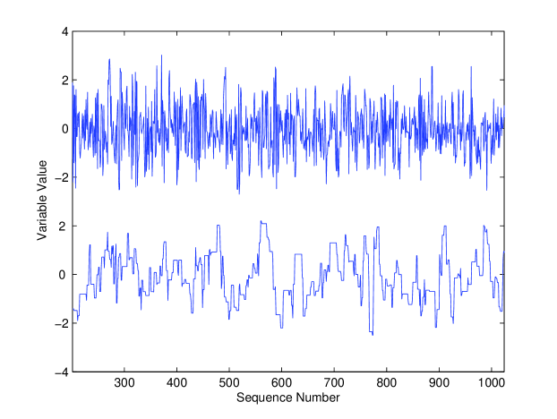
A 6-dimensional Gaussian distribution (as given above) with $\sigma_{0}=1$ is sampled with a chain of length $N_{samples}=8192$ using two methods: the Hamiltonian Monte Carlo method with $N=100$ leapfrog steps taken at each iteration at a step-size chosen such that $N\epsilon=\sigma_{0}$, and a Metropolis algorithm that uses a Gaussian proposal distribution with a step-size $\sigma_{T}/\sigma_{0}\approx 2.4/\sqrt{D}$.

Fig. 1 shows the chains generated by the two algorithms. These chains are used to compare the two methods. The acceptance rate for the HMC is $99\%$ while it is $25\%$ for the MCMC. HMC improves the mixing by accepting independent samples $4$ times more than the traditional MCMC chain. Correlations between the successive steps in these methods are shown in Fig. 2. The small panel shows the autocorrelations: the HMC autocorrelation dies off much faster than that of the MCMC. This feature is seen much better in the power spectrum of the chains. The HMC takes a smaller time to enter the white-noise regime at large scales than MCMC. This is given by the scale on which the power spectrum turns over and becomes flat which is around $k=0.1$ for the HMC and $k=0.02$ for the MCMC.

Figure 2: Power spectrum, $P(k)$, for the Hamiltonian Monte Carlo (solid red line) compared to that of a traditional MCMC method with an optimal step-size (dashed blue line).

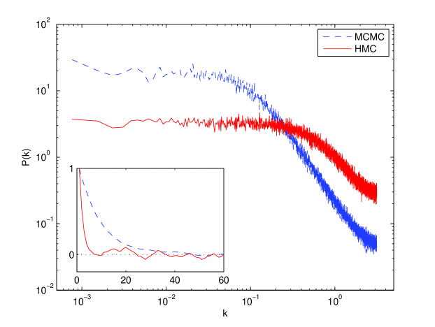
The efficiency of the chains can be read directly from the power spectra of Fig. 2. The efficiency is given by $\sigma_{0}/P_{0}$ and since $\sigma_{0}=1$, it is simply equal to $1/P_{0}$. The ratio of efficiencies are

$$\frac{E_{HMC}}{E_{MCMC}}=\frac{P_{0}^{MCMC}}{P_{0}^{HMC}}\approx 6.$$ (26)

Therefore in 6 dimensions an MCMC chain is 6 times longer than an HMC chain yielding the same performance. Later we will show that this number scales as the number of dimensions and hence the HMC does better than the MCMC on higher dimensions.

Figure 3: Marginalized distributions and two-dimensional contour plots of the 6-dimensional Gaussian model sampled with chains of length $N_{samples}=8192$ using the HMC (left) and MCMC (right).

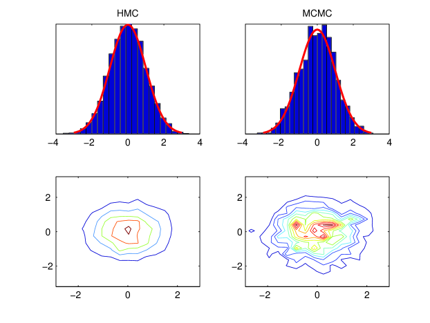
This can be seen more clearly in Fig. 3, where histograms of marginal distributions and two-dimensional contour plots are plotted for the both chains. For the same length of chains, the HMC gives more accurate results.

IV.1 Efficiency of the HMC

The exercise above can be repeated for other dimensions to see how the efficiency of the HMC chains are scales with the number of dimensions of the problem of interest. This can be done in two ways

1. by comparing the sample mean variance to an ideal chain; eqn.(22),

2. by computing the power spectrum and deriving the $P(k=0)$; eqn.(23).

We computed the efficiency of the HMC using the first method and cross checked it with the second method to confirm our results. The analysis are done for the HMC algorithm with $N\epsilon=1$. The efficiency is plotted versus the number of dimensions in Figure 4 and shows that it remains constant even in high dimensions.

Figure 4: Average efficiency of the HMC vs. the number of dimensions.

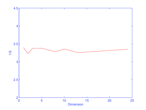
As a comparison, the optimal efficiency of the MCMC method is inversely proportional to the number of dimensions; $E\approx{1\over 3.3D}$ Dunkley:2004sv . And hence the ratio of the two efficiencies is proportional to the number of dimensions

$$\frac{E_{HMC}}{E_{MCMC}}\approx D.$$ (27)

Therefore in $D$-dimensions an HMC chain is $D$ times shorter than an MCMC chain yielding the same performance.

IV.2 Non-Gaussian And Curved Distributions

In 2 or more dimensions, the distribution of our interest may be very complicated. Sampling from non-Gaussian or curved distributions can be difficult and inefficient. In these cases usually a re-parametrization of the problem helps a lot to transform the distribution to a relatively simpler one which is easier to sample from Verde:2003ey .

Figure 5: left: The first 1000 samples drawn from the crescent-like distribution of eqn. 28 and their power spectra, $P(k)$ (right).

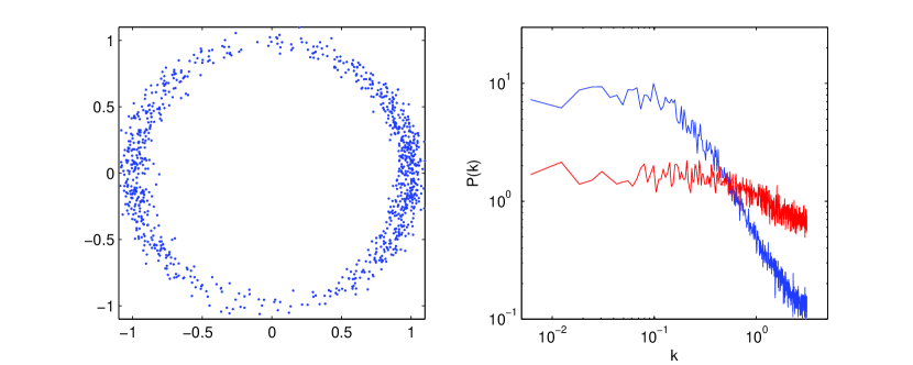
The HMC can improve the efficiency of sampling from these distributions. To demonstrate this, we choose the worst case scenario of Dunkley:2004sv ; a thin, curved, non-Gaussian distribution given by

$$E=\frac{(x^{2}+y^{2}-1)^{2}}{8\sigma_{1}^{2}}+\frac{y^{2}}{2\sigma_{2}^{2}}.$$ (28)

Sampling the above distribution in the present form is very inefficient with the traditional MCMC methods Dunkley:2004sv . In contrast, the HMC can easily sample that. Figure 5 shows the first 1000 samples drawn from the above distribution and their power spectra. The widths are chosen such that the dimensionless parameter $\sigma_{2}^{2}/\sigma_{1}=5$. As it can be seen in the figure, the chains have reached the equillibrium shortly and are sampling from the desired distribution. This is an idealized case where we exactly know the gradient at every point in the parameter space. However in a real-world problem we don’t know the gradients very accurately. We will discuss this in the next section and by applying this method to cosmological parameter estimation we will show that even a simple guess of the gradients will work. But better guesses will result in more efficient estimations.

V Cosmological Parameter Estimation with Hamiltonian Monte Carlo

The HMC is shown to be very promising in reducing the length of Markov chains for a reliable inference. Hence, this method can potentially speed up the cosmological parameter estimation by reducing the number of samples of a Markov chain. Taking a closer look at a typical algorithm for parameter estimation we will see the bottle necks of these algorithms are

1. Computing the power spectrum: at each step the CMB power spectrum should be computed for the new set of parameters. As the new experiments push to the larger $l$, computing the power spectrum becomes more time consuming.

2. Computing the likelihood: at each step, given the power spectrum, the likelihood should be computed. This is not as slow as the power spectrum computation, but becomes a bottle neck in long chains.

3. Number of samples needed in Markov chains: usually long Markov chains must be generated to achieve reliable results. Two practical issues of the MCMC chains are high correlations and low efficiency that result in long burn in times and high rejection rate. Specially in high dimensions, very lengthy Markov chains are needed (the ‘curse of dimensionality’).

The first two problems have attracted a lot of attention recently and fast methods of computing the power spectrum and likelihood have been designed Jimenez:2004ct , Fendt:2006uh and Auld:2006pm . All of these methods try to speed up the parameter estimation by making each step taken in a shorter time, but due to the nature of the traditional MCMC methods, still long chains are needed to obtain reliable results. An orthogonal and complimentary approach is to reduce the length of the Markov chains. This can be done by the HMC method. HMC can be done in ordinary cosmological parameter estimation codes. The method is simple and it is straightforward to add a module to a standard cosmological parameter estimation package, like CosmoMC, to perform that. The HMC algorithm needs to compute the gradient of the minus logarithm of the likelihood in each step. This can be done using an auxiliary distribution that mimics the minus logarithm of the likelihood function but is fast to compute. The leapfrogs can then be taken with no major additional cost of time.

V.1 Computing The Gradients: Zeroth Order Approximation

The simplest choice for an auxiliary function to estimate the gradients of the minus logarithm of the likelihood is

$$\frac{\mathcal{L}-\overline{\mathcal{L}}}{\sigma_{\mathcal{L}}}=({\bf x}-\overline{{\bf x}})^{\dagger}C^{-1}({\bf x}-\overline{{\bf x}}),$$ (29)

and the gradient would be

$$\frac{\partial\mathcal{L}}{\partial x_{i}} = \sigma_{\mathcal{L}}\left(\tilde{C}_{ij}^{-1}(x_{j}-\overline{x}_{j})+(x_{j}-\overline{x}_{j})\tilde{C}_{ji}^{-1}\right)$$

$$= \,2\,\sigma_{\mathcal{L}}\,\tilde{C}_{ij}^{-1}\,(x_{j}-\overline{x}_{j}).$$

As an example we sample from the 6-parameter flat LCDM model using the HMC. An exploratory run of traditional MCMC can be performed to obtain the fitting parameters $\sigma_{\mathcal{L}},\overline{\mathcal{L}}$ and $\overline{\mathbf{x}}$. Using the simple MCMC option of CosmoMC (sampling_method=1 option is to use the default Metropolis algorithm in the optimal fast/slow subspaces) at the exploratory phase the following fit to the minus logarithm of the likelihood is found

$$\mathcal{L} \simeq ({\bf x}-\overline{{\bf x}})^{\dagger}C^{-1}({\bf x}-\overline{{\bf x}})\sigma_{\mathcal{L}}+\overline{\mathcal{L}}$$

$$= \,0.5164\,({\bf x}-\overline{{\bf x}})^{\dagger}\,C^{-1}\,({\bf x}-\overline{{\bf x}})\,+\,5626,$$

where $C_{ij}$ is the covariance matrix and $\overline{\mathbf{x}}$ are the means, all estimated from the exploratory chains. These are all we need, the gradient can then be estimated using eqn. (V.1). Running modified CosmoMC with the above sampling method, yields $81\%$ acceptance rate. Proposed steps are rejected $19\%$ of times because of the imperfect estimate of the gradient of the field which causes inaccurate simulation of Hamiltonian dynamics. Even this simplest choice of the auxiliary function improves the acceptance rate by more than a factor of $3$ and reduces the correlations which in turn boosts up the efficiency of the chain and reduces the burn in time. However, this can be further improved to achieve a close-to-ideal sampler.

V.2 Computing The Gradients: Using Lico

Figure 6: Gradients of the minus logarithm of likelihood computed at 85 random positions using a Gaussian approximation to the likelihood and modified Lico.

A good feature of the HMC is that we are not limited to Gaussian auxiliary functions to estimate the gradients from. Hence we can choose functions that better resemble the minus log likelihood function. For example a polynomial fit can be made in the following form

$$\frac{\mathcal{L}-\overline{\mathcal{L}}}{\sigma_{\mathcal{L}}} = c_{0}+c_{1}(\frac{x_{1}-\overline{x}_{1}}{\sigma_{1}})+c_{2}(\frac{x_{2}-\overline{x}_{2}}{\sigma_{2}})+c_{3}(\frac{x_{1}-\overline{x}_{1}}{\sigma_{1}})(\frac{x_{1}-\overline{x}_{1}}{\sigma_{1}})$$

$$+ c_{4}(\frac{x_{1}-\overline{x}_{1}}{\sigma_{1}})(\frac{x_{2}-\overline{x}_{2}}{\sigma_{2}})+c_{5}(\frac{x_{2}-\overline{x}_{2}}{\sigma_{2}})(\frac{x_{2}-\overline{x}_{2}}{\sigma_{2}})+\cdots.$$

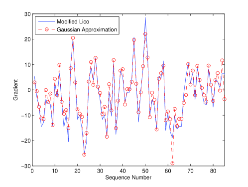
The coefficients of the above equation are found by Lico, the likelihood routine of the Pico package Fendt:2006uh . Lico breaks the parameter space into 30 regions and performs a fourth order polynomial fit to the $\mathcal{L}$ in each region separately. It is possible to modify Lico to compute the gradient of the above equation. This method must give a much better estimate of the gradients comparing to the simplest one.

Figure 7: Binned power spectra, $P(k)$, of the Markov chains sampled from the 6-parameter flat LCDM model using the default Metropolis algorithm of CosmoMC (dashed blue line) and the HMC (solid red line). The ratio of efficiencies are given by the inverse ratio of $P(0)$ for each method. The HMC is almost a factor of $6$ more efficient than the default Metropolis algorithm of CosmoMC. Autocorrelation functions for $\Omega_{b}h^{2}$ chains are also plotted in the small panel for comparison.

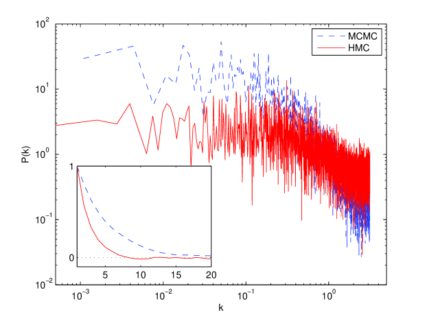
Fig. 6 shows the differences between the gradients computed using the two methods. Comparison is done at 100 random points in the parameter space.

To use this method in the HMC, we have added a module to CosmoMC that allows CosmoMC to use the above method based on Lico to compute the gradient of $\mathcal{L}$ whenever the parameters are within the range over which Pico s regression coefficients are defined. For parameters outside this range, CosmoMC will continue to use the Gaussian approximation to compute the gradient.

V.3 A Comparison between the HMC and the Monte Carlo method of CosmoMC

	$\Omega_{b}h^{2}$	$\Omega_{c}h^{2}$	$\theta$	$\tau$	$n_{s}$	$A_{s}$	Average
MCMC	11.5	19.6	11.7	28.9	17.8	13.5	17.1
HMC	3.2	2.8	4.0	2.9	3.4	3.8	3.3

Table 1: Autocorrelation lengths of the sampled chains from the 6-parameter flat LCDM model using the HMC and the Metropolis method of CosmoMC.

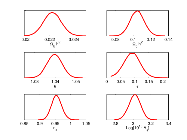
Having the HMC equipped with the above method of gradient estimation, we sample the 6-parameter flat LCDM model with an HMC sampler. The leapfrog step-sizes are the chosen to be $\epsilon=0.01\sigma_{i}$, where $\sigma_{i}=\sqrt{C_{ii}}$. We randomly draw the number of leapfrog steps taken at each iteration from a uniform distribution such that $N\,\epsilon\sim Uniform(0,3)\sigma_{i}$. We run the chain to generate $16000$ samples. This time we get $98\%$ acceptance rate, and very low correlations in the chain. We also run CosmoMC using the simple Monte Carlo option (with the optimal step-size $\sigma_{T}=2.4\sigma_{i}/\sqrt{D}$) to generate the same number of samples. The acceptance rate is $35\%$. The autocorrelation lengths of the HMC chain for the 6-parameter flat LCDM model are compared to those of the Metropolis method of CosmoMC in Table 1. The average autocorrelation length in the HMC chains are smaller than those of MCMC chains by a factor of $\sim 6$. This can be seen better in the power spectrum plots of Fig. 7. Autocorrelation functions are also plotted in the small panel for comparison. The efficiency of the HMC is almost an order of magnitude better than that of the default Metropolis method of CosmoMC. Therefore, using the HMC, one needs a much shorter chain to obtain the same accuracy as the Metropolis method.

Figure 8: Marginalized distributions of the 6-parameter flat LCDM model obtained from the HMC.

VI Discussion and Conclusions

With the future data of the upcoming experiments like ACT ACT and Planck Plank that will map the CMB sky on small scales (large $l$), the need to efficient and accurate methods of parameter estimation will be more. Besides finding methods of speeding up power spectrum and likelihood calculation, it is useful to design efficient Markov Chain Monte Carlo samplers to do reliable estimations with shorter chains.

We introduce the Hamiltonian Monte Carlo method (HMC) to improve the efficiency of the MCMC methods used in Bayesian parameter estimation in Astrophysics. This technique is based on Hamiltonian dynamics instead of the random walk. Hamiltonian dynamics allows the chain to move along trajectories of constant energy, taking large jumps in the parameter space with relatively inexpensive computations. This improves the acceptance rate and at the same time decreases the correlations among the chains. Unlike the traditional MCMC methods, the efficiency of the HMC remains constant even at large dimensions. Therefor shorter chains will be needed for a reliable parameter estimation comparing to a traditional MCMC chain yielding the same performance. Besides that, the HMC is well suited to sample curved, multi-modal and non-Gaussian distributions which are very hard to sample from using the traditional MCMC methods.

In addition to idealized toy models, we have applied this technique to cosmological parameter estimation. Our results have been compared to the outputs of the standard package of CosmoMC. For the 6-parameter flat LCDM model, the HMC is almost a factor of $10$ more efficient than the default MCMC method of CosmoMC. Therefore, using the HMC, one needs a much shorter chain to obtain the same accuracy compared to the Metropolis method.

In addition to the high efficiency, another important feature of the HMC is that we don’t have to compromise on the accuracy of our calculations. No approximation is made and the HMC sampler faithfully samples from the target distribution. It is shown in this paper that even a rough estimate of the gradient of the logarithm of likelihood can be used to make the HMC work. But the better the gradients are estimated the higher the acceptance rate will be. Combining this with methods of speeding up power spectrum and likelihood calculation such as Pico will make the Bayesian parameter estimation unbelievably fast.