Recovering the star formation rate in the solar neighborhood

This paper develops a method for obtaining the star formation histories of a mixed, resolved population through the use of color-magnitude diagrams (CMDs). The method provides insight into the local star formation rate, analyzing the observations of the Hipparcos satellite through a comparison with synthetic CMDs computed for different histories with an updated stellar evolution library. Parallax and photometric uncertainties are included explicitly and corrected using the Bayesian Richardson-Lucy algorithm. We first describe our verification studies using artificial data sets. From this sensitivity study, the critical factors determining the success of a recovery for a known star formation rate are a partial knowledge of the IMF and the age-metallicity relation, and sample contamination by clusters and moving groups (special populations whose histories are different than that of the whole sample). Unresolved binaries are less important impediments. We highlight how these limit the method. For the real field sample, complete to $M_{V}<3.5$, we find that the solar neighborhood star formation rate has a characteristic timescale for variation of about 6 Gyr, with a maximum activity close to 3 Gyr ago. The similarity of this finding with column integrated star formation rates may indicate a global origin, possibly a collision with a satellite galaxy. We also discuss applications of this technique to general photometric surveys of other complex systems (e.g. Local Group dwarf galaxies) where the distances are well known.

1 Introduction

Since the pioneering works of Bahcall & Soneira (bah (1984)) and Gilmore & Reid (gil83 (1983)), the comparison with deep star counts has been a primary method to disentangle the stellar components of the Milky Way. However, the number of parameters and the observational uncertainties involved in this kind of analysis are often prohibitive. In contrast, nearby stars are a well defined sample of disk stars and the distances are now well known so one can extract detailed information about the local star formation rate and how this is connected with the whole Galactic disk.

In this framework, the Hipparcos catalog provides a unique opportunity. Before Hipparcos, the local stellar population of bright stars, in main sequence or in red giant phase, was poorly represented; moreover, the distance uncertainties washed out most of the fine structure of the color-magnitude diagrams (CMDs). After Hipparcos, it was possible to study the color-magnitude diagram for local stars in a statistical sense, beyond the simple comparison between evolutionary tracks and single stars, a method for which is the subject of this paper.

Published studies based on the Hipparcos local sample have concentrated on two approaches. One is the direct comparison between data and artificial CMDs using a likelihood function, e.g. Bertelli & Nasi (bert (2001)) and Schröder & Pagel (scho (2003)). The second is the Bayesian approach, e.g. by Hernandez et al. (her2 (2000)) and Vergely et al. (verg (2002)).

Here we suggest an hybrid technique (for an over-complete description see Cignoni 2006). First, we adopt a Bayesian treatment of the observational uncertainties: the CMD is converted into an image (binning process) and a Richardson-Lucy algorithm is used to clean the data (see Cignoni & Shore 2006 for details). This “cleaned” Hipparcos CMD can then be used to recover the local star formation rate (SFR). This is done in different steps, as described in the following sections: (1) an ensemble of synthetic CMDs is generated using Monte Carlo simulations; (2) a likelihood function is minimized for the comparison between theory and observation; and (3) a confidence limit of the result is evaluated with a bootstrap technique.

In section 2 we describe the properties of the selected volume complete sample and how we removed the known stellar clusters, moving groups, and associations. Sections 3 and 4 describe the method: physical inputs adopted for the stellar evolutionary calculations, Monte Carlo generations of artificial CMDs, likelihood function and bootstrap. In section 5 we apply the algorithm to artificial CMDs, showing which parameters are critical for recovering the star formation rate. Section 6 shows the results for the Hipparcos data. Section 7 discusses the dependence of the recovered SFR from a kinematic selection of the data. Finally in section 9 the results are discussed and compared with previous works available in the literature.

2 Sample selection

The Hipparcos mission observed objects to a limiting magnitude of about $V=12.5$ mag, with a completeness limit that depends on Galactic latitude $b$ and spectral type (see e.g. Perryman et al. per (1995)): $V<7.9+1.1\sin|{b}|$ for spectral types earlier or equal to G5, $V<7.3+1.1\sin|{b}|$ for spectral types later than G5.

For a volume complete sample, we chose stars within 80 pc of the Sun and brighter than $V=8$ in visual apparent magnitude, corresponding to a minimum absolute visual magnitude $M_{V}=3.5$. Considering that the formal completeness limit is dependent by galactic latitude and spectral type, we checked if the sample is still complete against the Malmquist bias (in a magnitude limited sample, the brighter stars are statistically over-represented). The bias was quantified by comparing the luminosity functions for subsamples with different heliocentric distances. Figure 1 shows the luminosity functions for stars with different distances from the Sun at intervals of 10 pc.

Figure 1: Luminosity functions (in absolute visual magnitude) for stars selected in distance (as labeled). All the stars are brighter than $V=8$.

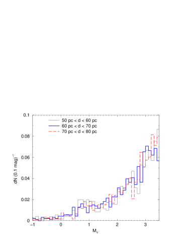
Using a Kolmogorov-Smirnov test, the hypothesis that the luminosity functions are realizations of the same distribution (for the range $-1<M_{V}<3.5$) cannot be rejected with a probability of 10%. Thus, the sample selected at $V=8$ should be complete up to 80 pc and $M_{V}=3.5$, which is ensured by selecting Hipparcos stars that are brighter than $V\sim 8$ and within $80$ pc from the Sun. This sample contains about $4000$ objects with a parallax error generally better than 10% (see Fig. 2).

Figure 2: Distribution of the parallax precision ($\Delta\pi/\pi$) for Hipparcos stars within 80 pc and brighter than $V=8$.

2.1 Clusters contamination

We are interested in the local star formation activity as it reflects that of the whole disk. In contrast, nearby clusters and associations are groups of stars that are not dynamically mixed with the field and which - having been formed together in large numbers at specific times - do not represent the mean properties of the solar neighborhood. Figure 3 shows the identified associations members within 80 pc and brighter than $V=8$. The most significant contamination is by the Hyades cluster with about 120 identified members.

Figure 3: The selected Hipparcos sample where members of associations are shown.

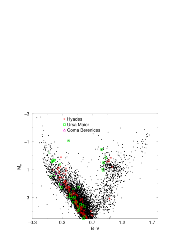
We will hence call “the Hipparcos sample” the set defined after that the identified cluster members are eliminated.

3 The model

3.1 Theoretical inputs

To recover the star formation history from the observational CMD one needs to model a synthetic population with various theoretical ingredients. Using a Monte Carlo algorithm (CERN library), masses and ages are extracted according assumed initial mass functions (IMFs) and star formation rates (SFRs). Then, a suitable age-metallicity relation (AMR) is adopted. The extracted synthetic stars are placed in the CMD by interpolation among the adopted stellar evolution tracks. In order to take into account the presence of binary stars, a chosen fraction of these stars are assumed as binaries and coupled with a companion star.

The code relies on a set of evolutionary computations covering with a fine grid the mass range $\approx\,0.1$ to $\approx\,7M_{\odot}$, with metallicities from $Z=0.001$ to $Z=0.03$. The amount of original helium abundance has been chosen by assuming a primordial helium abundance $Y_{P}=0.23$ and $\Delta Y/\Delta Z\sim 2$ (see e.g. Pagel & Portinari pag (1998), Castellani, Degl’Innocenti & Marconi cast99a (1999)). The adopted color transformation are from Castelli, Gratton & Kurucz (1997)

For masses greater than $0.5\,M_{\odot}$ we use the Cariulo et al. (car (2004)), Castellani et al. (cast03 (2003)), Castellani, Degl’Innocenti & Marconi (cast99a (1999)) evolutionary tracks (partially available at the URL: http://astro.df.unipi.it/SAA/PEL/Z0.html). The input physics adopted in the models are described in Cariulo et al. (car (2004)). Convective regions, identified following the Schwarzschild criterion, are treated with the mixing length formalism in which the mixing length parameter $\alpha$ defines the ratio between the mixing length and the local pressure scale height; we have uniformly adopted $\alpha=1.9$, which has been calibrated in a way to reproduce, with the adopted color transformations, the observed RG branch color of the galactic globular clusters and young globulars in the LMC (Cariulo et al. car (2004), Castellani et al. cast03 (2003), Brocato et al. broc (2003)). The solar mixture adopted for the calculations is $[Z/X]_{\odot}=0.0245$ (Grevesse & Noels greve (1993), GN93). We use throughout the canonical assumption of inefficient overshooting and the He burning structures are calculated according to the prescriptions of canonical semiconvection induced by the penetration of convective elements in the radiative region (Castellani et al. cast85 (1985)).

Less massive stars ($0.5\,M_{\odot}<\,M\,<\,0.7\,M_{\odot}$), whose evolutionary times are longer than the Hubble time, have been evolved up to central H exhaustion. For very low mass stars ($M<0.5\,M_{\odot}$) we used the Zero Age Main Sequence positions by Baraffe et al. (bar7 (1997),bar8 (1998)).

3.2 Artificial CMDs

The so called “forward” procedure for obtaining a SFR that can generate an observed photometric sample diagram is to produce artificial CMDs to be compared with the observations. The first technical problem of a similar approach is the time spent for the Monte Carlo generation of a CMD for each SFR. Both the data and the artificial photometry are stored in a color magnitude grid, each bin of which contains the number of stars observed or predicted to be in it. The SFR with the higher probability of generating the data is chosen by means of a likelihood test. So, to explore a sufficiently wide number of star formations, it is necessary to construct a basis set, each of partial CMDs with $\approx 10^{5}$ stars per step star formation, uniform in a given time interval and zero elsewhere. The step functions must be exhaustive (the sum covering the whole Hubble time) and they cannot overlap.

Thus, for each combination of IMF and AMR, the CMD corresponding to any SFR is computed as a linear combination of the partial CMDs:

$$m_{i}=\sum_{j}r_{j}\,c_{ij}$$ (1)

where $m_{i}$ is the number of star in the final CMD in bin $i$, $r_{j}$ is the star formation rate for the partial CMD $j$, and $c_{ij}$ is the number of stars in the bin $i$ owning to the partial CMD $j$.

The number of Monte Carlo simulations is reduced to the number of partial CMDs. This method has been already applied by several authors (see e.g. Aparicio, Gallart & Bertelli 1997a -1997b , Gallart et al. gal (1999), Bertelli & Nasi bert (2001)). The duration of each star formation interval is chosen depending on the timescale of the typical stellar population involved, in order to properly sample even those stars with rapid evolutionary changes. Thus, we have chosen star formation steps of 0.5 Gyr for stars younger than 2 Gyr, while for the later epoches the duration is increased (1 Gyr for stars with age between 2 and 4 Gyr, 2 Gyr for older stars).

4 The comparison between theory and observation

4.1 Choosing the grid

Choosing the grid dimension for the CMD binning is an essential step. If the CMD bins are too small, the histogram fluctuations are too large and it’s more difficult to recover the underlying SFR. If the bin size is too large one can loose information.

A first rule for choosing the grid uses from the typical masses involved in the sample: massive stars have shorter life time (and the corresponding CMD regions are underpopulated) and it is thus suitable to use a larger bin size in order to map their history. Another limit is the evolutionary phase of the star mapping the CMD: after the main sequence, the partial CMDs become nearly degenerate and consequently the grid needs to be finer. The adopted binning must arise by numerical simulations for the specific problem to check the sensitivity of the algorithm to the various choices.

4.2 Searching for the “best model”

To quantify the similarity among CMDs, we chose a Poisson based likelihood function:

$$\chi_{P}=\sum_{i=1}^{Nbin}n_{i}\ln\frac{n_{i}}{m_{i}}-n_{i}+m_{i}$$ (2)

where $m_{i}$ and $n_{i}$ are the model and the data histogram in the i-bin. This “likelihood” is considered as a mere “distance” to be minimized, while the acceptance level of a solution is estimated using a bootstrap technique.

Our model depends on several parameters (10 coefficients of the star formation rate), thus, the problem is to move within this multi-dimensional parameter space and to search for the combination of parameters that minimize $\chi_{p}$. For this task we implement the Nelder-Mead simplex method (Nelder & Mead, neld (1965)). The main problem of the simplex method is the efficency: the presence of many local minima can prevent reaching a real global minimum for $\chi_{P}$. To improve the efficency we add a logarithmically distributed random variable to each vertex of the simplex, the minimization algorithm is re-started each time a “global minimum” is found, and the new departure is randomly chosen (in order to avoid the dependence by the initial guess) in the parameter space to obtain a class of best values. The final best parameter is the smallest among the best values. The restart process is stopped when this “minimum value” no longer changes.

4.3 Confidence intervals

The bootstrap method is commonly used to estimate confidence intervals. In empirical bootstrap simulations one processes the original data set $N$ times (copies) so each of the original $n$ data points is sampled with replacement and with equal probability of being sampled. One finally obtains $N$ different data sets, each with $n$ data points. Because of the replacements, some values in each data set are repeated, while others are lacking. This mimics the observational process: if the observational data is representative of the underlying distribution, the data produced with replacements are copies of the original one with local crowding or sparseness. In practice, the method uses the bootstrapped copies imposing the same minimization procedure as it would be performed on the real data set. The result will be a set of “best” parameters. The confidence interval is then the interval that contains a defined percentage of this parameter distribution.

5 Sensitivity tests with artificial data

Applying the method to artificial data, we have tested:

1. how the completeness limit, that fixes the boundaries in magnitude of the CMD used for the analysis, affects the result. Different zones in the CMD give information about different epochs of star formation. The completeness limit determines our “zone of ignorance” for the underlying SFR.

2. how sensitive the recovered SFR is to parametric functions such as the IMF, AMR, binary population. This procedure may highlight parameters whose values need to be known very accurately in advance;

3. how the contamination of accidental intruders (e.g. stellar cluster stars) in the sample, could lead to a biased SFR.

For all tests we have fixed the grid bin size. Young partial CMDs comprise massive stars so the spanned region is broad (the more massive the star is, the longer its excursion in color to reach the red giant branch) and poorly populated: small bins contain few stars and the recovered SFR suffers of low number statistics. Old partial CMDs are composed by less massive stars so a narrower bin size is required to distinguish different SFRs. After some trials we found that a bin size of 0.05 mag, both for the color and absolute magnitude, is the best compromise. Hereafter, we call “artificial data” each synthetic CMD mimicking the Hipparcos data while the theoretical CMD is simply called the “model”.

5.1 Completeness limits

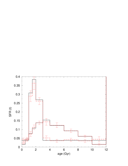
The completeness limit of the observed CMD limits our ability to exploiting all the information contained in the CMD. In this section we explore how different limits in absolute magnitude can modify the recovered SFR. We analyze three different completeness limits: $M_{V}=2.5,3.5,4.5$. During the test we separately select the contribution given by main sequence stars and later evolutionary phases (RGB and red clump), defined as stars with $B-V>0.8$. The results are drawn in Fig. 4 (here and in the following all SFR histograms have unit area).

Figure 4: “True” (solid line) and recovered (dashed line) SFR from stars brighter than $M_{V}=2.5,3.5,4.5$. On the left the figures show the results obtained using only main sequence stars. The figures on the right represent the recovered SFR by including all the evolutionary phases.

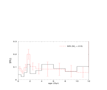
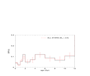
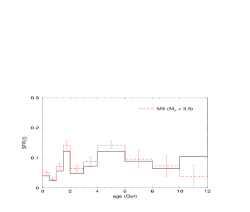
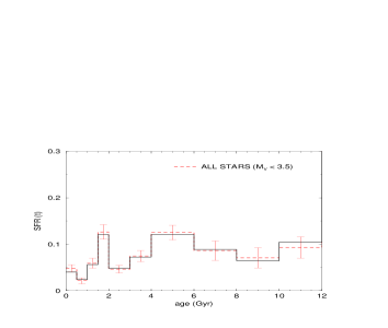
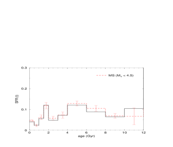
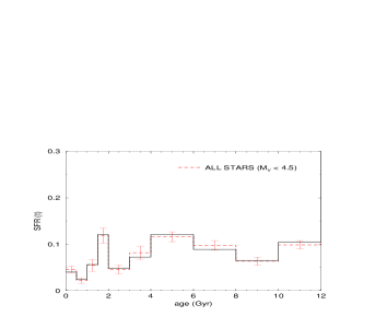
Main sequence stars with $M_{V}<2.5$ mag give information about only the recent SFR, while we learn nothing about stars older than 3 Gyr (this is evident from the large error bars for the recovered SFR beyond this age, which mitigates the result and demonstrates the impossibility for the procedure to recover the SFR due to the lack of information). The result is significantly improved by also including later evolutionary phases. The recovered SFR is close to the original one, even if the error bars are quite large. This is due to the fact that one obtains information only from fast evolutionary phases (clump and red giants for the past star formation and upper main sequence for the recent one) and the probability of finding stars in these zones is low. Obviously we are considering a perfect situation where both the chemical composition and the IMF of the stars are well known so the uncertainty is as minimum as possible; for real data other sources of uncertainties occur. Including stars to $M_{V}=3.5$ the precision of the recovered SFR increases and from the main sequence alone one can obtain the SFR up to $\sim 6$ Gyr. However, to study earlier epochs it is needed to include later evolutionary phases. Also in this case the uncertainty in the recovered SFR, for stars older than 6 Gyr, is large. The reason is the same: for $M_{V}<3.5$, the information on the ancient star formation comes only from late evolutionary phases which are too rapid to provide for a large number of stars. By increasing the magnitude limit at $M_{V}=4.5$, the entire SFR is recovered with small uncertainties. The inclusion of the main sequence, however, produces a systematic difference between the input and recovered SFR for the oldest era while including late evolutionary phases leads to the right solution.

This finding is easier to understand if one looks how different masses contribute to different epoches of star formation. Figures 5 draw this map (for minimum luminosities $M_{V}=3.5$ and $4.5$) for an artificial population built with a constant SFR (0-12 Gyr) and Salpeter IMF.

Figure 5: Theoretical distributions in time of stars generated with a flat SFR (0-12 Gyr), Salpeter IMF and solar composition. Different lines indicate different mass ranges. In the upper panel only stars with visual absolute magnitude below 3.5 are plotted, while in the lower panel the magnitude limit is $M_{V}=4.5$.

If the minimum luminosity is set to $M_{V}=3.5$ we cannot see the main sequence for masses below $1.2\,M_{\odot}$. So this mass range the RGB and He burning stars provide information about the earlier epochs, but not on the recent SFR. At $M_{V}=4.5$ we see the main sequence down to $1\,M_{\odot}$, so we can analyze with this mass range each period between now and $10-12$ Gyr ago. These results are not linked to the particular SFR parameterization: Fig. 6 shows the recovered SFR for different input SFRs.

Figure 6: As in Fig. 4 for $M_{V}<4.5$ and all evolutionary phases for different input SFR shapes.

In the following we present test results involving artificial data adopting the magnitude limit $M_{V}=4.5$.

5.2 IMF - SFR degeneracy

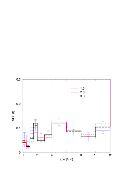
Even if the form of the IMF is well defined for masses above $1\,M_{\odot}$ from observations and theoretical analyses (see e.g. Larson et al. lars (1992)), the precise value of the exponent is still debated. For instance, Kroupa (krou (2001)) finds the Salpeter exponent 2.3$\pm$0.7 to be the most likely value, and any study of the local SFR must account for this uncertainty.

The possibility that changes in the IMF mimics the SFR effects on CMD is a well known degeneracy. We analyzed the sensitivity of the recovered SFR to the chosen IMF using different IMF exponents ($s=1.3,\,2.3,\,3.3,\,4.3$) for the artificial data while in the model a fixed IMF exponent equals to 2.3 was used. The results are shown in Fig. 7. It’s noteworthy that the input SFR is always recovered: even if a wrong IMF is adopted (that is, different from the one used for the artificial data), it doesn’t lead to a wrong solution (at least for “reasonable” IMF exponents less than 4). In conclusion, for the mass range covered by Hipparcos sample ($M_{V}\leq 4.5$), the IMF exponent alone is not a crucial parameter if the AMR is known in advance. Figure 5 shows this. For ages $<6$ Gyr the CMD is populated by the whole mass spectrum (only very massive stars are dead), so a variation of the IMF modifies the population in this age range in the same way (the relative SFR is preserved). In contrast, the old eras (8 to 12 Gyr) include only low mass objects (even intermediate mass stars are already dead), thus the IMF variations mainly alters the ratio between old (older than 8 Gyr) and recent star formation (see Fig. 7).

Figure 7: The “true” (solid line) and the recovered SFR for different values (labeled) of the IMF exponent used in the artificial data. The IMF exponent used in the model is fixed to 2.3.

5.3 Binaries - SFR degeneracy

Another source of uncertainty, when one looks at the solar neighborhood, is the percentage of stars in unresolved binary systems. Our model doesn’t account for binary evolution with mass exchange: we assume that each binary component evolves as a single star. Our knowledge of binary stars populations and evolution in the local disk is far from perfect, so including interacting binaries in the simulations would involve many unknown parameters (such as the mass exchange rate, evolution of the separation, etc.). However, the mere presence of a given percentage of unresolved binary systems affects the CMD morphology. In order to perform this analysis, we have built the usual artificial data using different prescriptions on the binary population (10%, 30%, 50% of binaries with random and equal mass ratio). The partial CMDs used in the model are built with the same composition and IMF adopted for the artificial data, but without binaries. The results of the simulations are shown in figure 8. As found for the IMF, if the mass ratio is uniformly distributed, we can recover the correct SFR independently on the presence of binaries. In the extreme case of equal mass ratio ($q=1$), the recovered SFR is severely biased. In particular, the presence of binaries doesn’t affect the recent result, while the only modifications affect the old SFR.

Figure 8: “True” (solid line) and recovered SFRs. The artificial data is generated with the indicated percentage of binaries and mass ratio (random number or unity), while the model is without binaries.

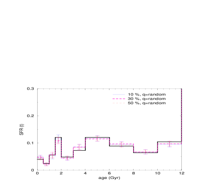
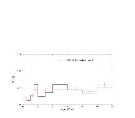
The explanation comes from the displacement that binaries cause from single star CMD: if the mass ratio is uniform the smearing effect is random and the main sequence is merely wider (this effect is generally smaller than 0.05 mag, which is the binning size) and it looks like an increased photometric error for the recovered SFR. If, however, the mass ratio is unity, the global effect is systematic and the main sequence develops a parallel double: in this case the recovered SFR is systematically biased. Thus, to recover a star formation rate, the choice of the binary population is not crucial but if an extreme prescription is adopted (e.g. equal masses), the recovered SFR may be biased.

5.4 Metallicity - SFR degeneracy

An old, metal-poor stellar populations can mimic younger, metal-rich populations. Moreover, knowing that the solar neighborhood is a mix of stars of different chemical compositions (see e.g. Nordström et al. nord (2004)), we expect a very complex influence of the composition on the CMD morphology. These simple considerations oblige us to check if it’s still possible to recover the SFR when only a partial knowledge on the age-metallicity relation is available.

In these calculations we now assume that the IMF and the binary population are the same both in the model and in the artificial data.

5.4.1 Artificial data with single metallicity

As first step, we have built an artificial population with a single metallicity (no AMR), then, the SFR is recovered assuming a wrong metallicity. The results are shown in Fig. 9.

Figure 9: Sensitivity test to metallicity. The adopted composition for the model is solar. If the data have the same composition, the “true” SFR (heavy solid line) is close to the recovered one (heavy dashed line). If the data metallicity is slightly different from the solar value ($\Delta Z=\pm 0.005$), systematic relevant deviations appear in the solution.

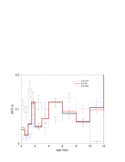
If we adopt the same metallicity for the artificial data and for the model, the SFR is recovered. However, if we slightly change the metallicity in the data ($\Delta Z=\pm 0.005$), without changing the composition of the model, systematic discrepancies appear in the recovered SFR. If the artificial data are metal poor compared to the model, the recovered old SFR is underestimated (and the recent one is overestimated) and oppositely for metal richer artificial data. This result is a strong warning about the widely used assumption of solar composition for nearby stars: small deviations from the solar value could bias the derived SFR. Moreover, we know that deviations from solar values exist and are usually much larger than $\Delta Z=\pm 0.005$. Figure 10 shows the age-metallicity relation and the metallicity distribution by Nordström et al. (nord (2004)), the most representative census for ages and metallicities in solar neighborhood. This is characterized by a constant mean metallicity and a large scatter at all ages (about $\sigma\sim 0.2\,\rm dex$ in $[Fe/H]$). The quoted formal error of $\sim 0.1$ dex in $[Fe/H]$ cannot account for the observed spread.

Figure 10: Left panel: age-metallicity diagram for single stars (within 40 pc from Sun) with age determination better than 25% (from Nordström et al. nord (2004)). Right panel: the distribution of $[Fe/H]$ for the same sample.

5.4.2 Artificial data with an age-metallicity dispersion

In order to test the sensitivity to a metallicity dispersion, artificial data were generated with the observed mean metallicity plus a variable dispersion (the explored range is from $\sigma=0.01$ dex to $\sigma=0.2$ dex in $[Fe/H]$). The conversion between $[Fe/H]$ and $Z$ that is appropriate for our models calculated for the GN93 composition ($[Z/X]_{\odot}=0.0245$) is:

$$\log Z=0.73\times 10^{([Fe/H]-1.61)}$$ (3)

The enhancement of $\alpha$ elements is not included because it has shown to be negligible for disk stars.

The SFR was searched, adopting in the model the same mean metallicity of the artificial data, but without metallicity spread. The results are shown in Fig. 11,

Figure 11: Solid line: SFR assumed for the artificial data. Dashed line: recovered SFR. The $\sigma$ value indicates the dispersion in $[Fe/H]$, used for the artificial data. The model has the same mean metallicity, but no dispersion.

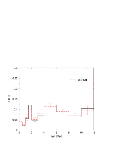
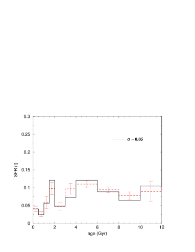
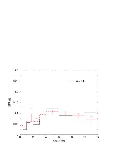
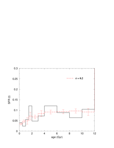
where the solid line is the input SFR and the dashed line the recovered one. Above $\sigma=0.1$ dex, most of the information contained in the SFR is lost: this numerical experiment has pointed out how the dispersion in metallicity can be a critical factor. A wrong estimate of the dispersion leads to a wrong solution.

For the final test we adopt the same dispersion both in the artificial data and in the model. The idea is to check if in presence of dispersion, even when we rightly estimate the metallicity dispersion of the data, the spread of the CMD due to the metallicity spread still allows to recover the underlying SFR. In order to do a realistic attempt, we adopt the metallicity distribution by Nordström et al. (nord (2004)) (Fig. 10).

The overall effect is a broadening of the partials CMDs. The SFR extraction is presented in figure 12 for an artificial population generated with this AMR.

Figure 12: Input SFR (solid line) compared with the recovered SFR (dashed line). Model and artificial data have the same metallicity dispersion.

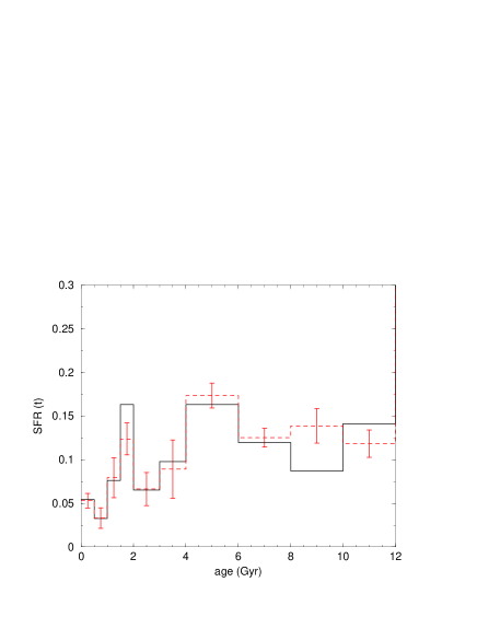
There are systematic shifts between the recovered and the input SFRs, indicating a limit in our ability to distinguish different stages of star formation (for a comparison with the single metallicity tests, see section  5.4.1), but the trend is preserved. The implication for real data is actually encouraging: if the nearby stars show an age-metallicity relation like the Nördstrom et al. result, the application of the model to Hipparcos stars can give information on the real SFR.

5.5 Contamination from clusters and associations

The solar neighborhood includes stellar clusters or part of them. We have removed about 80 stars (mainly Hyades stars) within 80 pc and brighter than $M_{V}=3.5$. This number may appear small ($\sim 2\%$ of the total sample), but these object are concentrated in time so they can produce a burst in the SFR (at $\sim 0.5$ Gyr, for the Hyades) which does not represent a galactic field property.

However, we cannot exclude that some cluster members remain as yet unidentified, so an interesting analysis involves the cluster impact on the recovered SFR. We have contaminated an artificial sample with a variable percentage of synthetic Hyades-like stars (500 Myr and solar metallicity), from 2% to 15%, with the results shown in Fig. 13. At 2% contamination the SFR changes within the error bars. Increasing the cluster percentage, the peak at 500 Myr becomes progressively more evident. At 15%, the recovered SFR is perturbed on a scale of 5 Gyr.

Figure 13: Recovered star formation rates for different contaminations (the percentage is labeled) of Hyades-like stars.

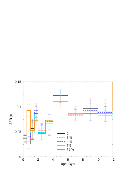
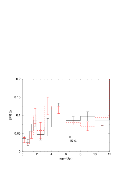
The same test has been performed with a synthetic cluster at 2 Gyr. Figure 14 shows the recovered SFR when 15% of synthetic cluster stars is added to the artificial data. It is evident that the changes in the recovered SFR are not isolated at 2 Gyr, but the whole SFR shape between 2 Gyr and 7 Gyr is altered.

Figure 14: Solid line and dashed line are respectively the recovered SFR when the contamination by cluster stars (2 Gyr old) is 0 and 15%.

6 Comparison with real data

We are now ready to present the SFR extraction from the real Hipparcos data. Because both the IMF and the binary population are not crucial factors (see sections  5.2 and  5.3), we have fixed them: the IMF exponent is Salpeter, there are no binaries, and we have again assumed the Nordström et al. AMR. Before applying the SFR extraction method to real data, we must treat the observational errors. Cignoni & Shore (2006) show how the Richardson-Lucy algorithm allows to restore the original CMD corrupted by a point spread function. Here, we apply the SFR extraction to the Hipparcos CMD that was previously deconvolved by this algorithm. However, the result of a R-L restoration is a two dimensional histogram and the information on the single stars is lost. Thus we cannot directly apply the bootstrap technique to determine the variance on the recovered SFR. A trick to avoid this problem is to construct bootstrap replicates of the data before the Richardson Lucy restoration. Then each bootstrap data is reconstructed with the R-L algorithm and the SFR is obtained for each reconstruction. This set furnishes the mean and variance for the final SFR.

The R-L algorithm is performed with the PSF built from the observational absolute magnitude error distribution. Figure 15 shows the results: the different curves represent the recovered SFR, after respectively 5, 10, 15, 20, 25 R-L restorations. In order to avoid artifacts, the restoration is stopped at the 25-th iteration when the bulk of the restoration is done (see discussion in Cignoni & Shore cign (2006)). For comparison, Fig. 15 (upper panel) shows the recovered SFR (labeled with 0) when our method is applied to the data without R-L restorations.

Figure 15: The SFR recovered from the Hipparcos sample. The comparison area involves all stars brighter than $M_{V}=3.5$. Different lines show the result after the labeled number of R-L iterations.

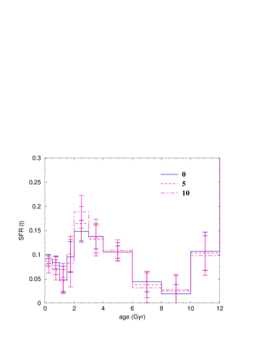
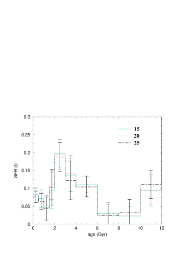
The global effect of the restorations is small and it is most evident around 2-3 Gyr. Over the 10th iteration, the solution is very stable and the only change is the increase of the estimated uncertainties because of the noise amplification.

Before discussing the recovered SFR, it is necessary to recall that the implemented Nordström et al. AMR is uncertain for ages lower than 1.5 Gyr and greater than 7 Gyr, thus the result for these ages could be unavoidably biased. Moreover, all the information (at $M_{V}<3.5$) on the SFR older than 7 Gyr comes from evolved stars, with the associated under-population problems. All these points will be discussed further. For the moment, we describe the results for the SFR:

• A bump in the time interval 10-12 Gyr;

• A modest activity in the time interval 7-10 Gyr;

• A steep increase from 2 Gyr to 6 Gyr;

• A modest activity during the last 1 Gyr.

In order to check the robustness of our finding, we tried to recover the SFR by adopting a different time resolution. In particular we tested a power law stepping $\delta t=[{(1+\varepsilon)^{n}}\,\times 0.5\,Gyr]$, with $\delta t$ the step duration, $\varepsilon$ a parameter and $n$ a running index (integer, starting from 0). Figure 16 shows the recovered SFR for $\varepsilon=1$.

Figure 16: The recovered SFR for a power law step resolution (dashed line; $\varepsilon=1$, see text) is compared with the result of Fig. 15. Both the SFR are obtained after 1 R-L restoration.

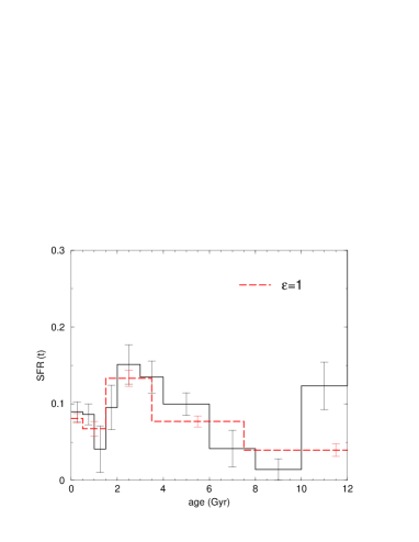
The coarser time steps allow to reduce the uncertainties, but the overall shape for ages less than 8 Gyr is confirmed. As we will discuss later, the results for greater ages are affected by many sources of uncertainty. In the following, the temporal resolution will be fixed to the prescription of section 3.2. Moreover the number of R-L restoration is fixed at 15.

6.1 Warnings about the AMR

Our SFR represents the most probable result provided that the model is not biased. As already discussed, the observed AMR is chosen mainly because it arises from a very wide observational sample. However, it is still affected by three important biases:

1. it was built looking for F-G type stars. This selection was done choosing stars between suitable blue and red color boundaries (by means of $(b-y)$ Strömgren color, which is almost metallicity independent). However, as a consequence of the blue cut-off, the younger metal poor stars are under-represented in the final AMR;

2. Due to the observational errors, the stellar age determination is progressively more and more difficult as a star is close to the zero age main sequence (where the stellar tracks degenerate). Consequently, the Nordström AMR is poorly known for very young stars and the AMR we used below 1 Gyr is an extrapolation;

3. The age determination is also a problem for stars older than 8 Gyr, because at these ages the main sequence is populated by low mass stars which evolve in a restricted region of the CMD. As a consequence, the ancient part of the AMR is given with very large uncertainties in the age (e.g. the presence of stars older than 13 Gyr).

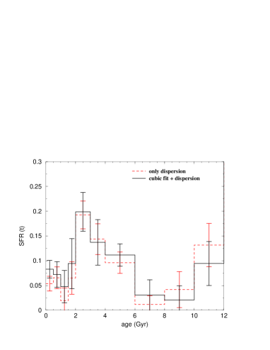
Although we have selected stars with a relative uncertainty for the age better than 25%, the previous points lead to doubts about the recovered SFR for stars younger than 1 Gyr and older than 8 Gyr. In particular, the recovered activity during the last 1 Gyr is partially due to the way the AMR is parameterized in our model. Figure 17 shows the effect of a different parameterization: the solid line is the resulting SFR if the adopted AMR is a polynomial fit (cubic) plus the dispersion, the dashed line is the result when the dispersion alone is implemented.

Figure 17: Dependence of the result on a different parameterization of the observed AMR. The dashed line indicates the SFR that is obtained implementing the metallicity spread of the Nordström et al. AMR. The heavy line indicates the resulting SFR when a cubic interpolation of the Nordström et al. data plus the same observed dispersion is adopted, see text.

6.2 Warning about the adopted completeness limit

Another point is the completeness limit $M_{V}=3.5$: in section 5 we showed how the information on the old SFR is enough limited by the completeness limit, with the full information only available with an hypothetical sample complete up to $M_{V}=4.5$. With the $M_{V}=3.5$ cut-off, the only tracers of the star formation older than 7 Gyr (see Fig. 5) are red giants, clump stars and subgiants. For this reason, at ages older than 7 Gyr the recovered SFR is certainly undersampled (see Fig. 18). Thus, the bump between 10 and 12 Gyr could be an artifact.

Figure 18: The highlighted region identifies the time interval where the recovered SFR is undersampled (because of the magnitude cut at $M_{V}=3.5$, the only tracers at these ages are red giant and helium clump stars).

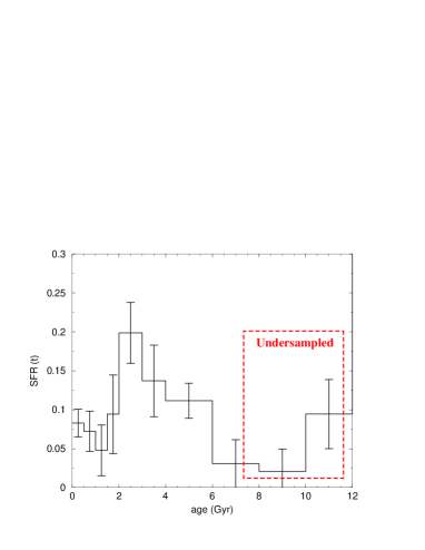
Only a deeper volume limited sample will provide a better understanding on the old SFR.

7 Kinematical selection

A genuine star formation rate should represent the number of stars born at each time in our volume; this condition can fall, for example when:

• Old disk stars may have diffused into a larger volume, so the old local SFR may be undersampled: the stellar velocities are randomized through chance encounters with interstellar clouds, they gain energy and increase the velocity dispersion.

• “Hot” populations may contaminate the sample. Thick disk and halo stars have kinematical properties that could have been fixed before the disk developed. These stars sample a much larger volume of the disk stars and they are weakly represented in the solar neighborhood.

In these cases, the recovered SFR would be a mere census of the ages of the stars actually present in the solar neighborhood. In order to avoid thick disk/halo contaminations and to check the amount of orbital diffusion of old disk stars, we have evaluated the Galactic velocity components for all stars in the sample and recovered the SFR for different kinematically selected subsamples.

The Hipparcos mission measured proper motions which, together with the parallaxes, give tangential velocities $V_{T}$. For most of the stars in our sample, a measured radial velocity is available (from the SIMBAD database ). With these data, we have computed the Galactic velocities U,V and W for more than 90% of the stars in the sample, corrected for the solar motion relative to the Local Standard of Rest (LSR, $U_{\odot}=+10.0$ Km/s, $V_{\odot}=+5.2$ Km/s, $W_{\odot}=+7.2$ Km/s according to Dehnen & Binney deh (1998)). Figure 19 shows the distribution of U,V and W velocities for all stars in the sample with measured radial velocities.

Figure 19: Distribution of U,V and W velocities (referred to the LSR) for all stars in the sample with a measured radial velocity and $M_{V}<3.5$.

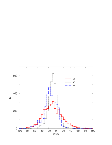
In order to search for stars with thin disk properties we need a kinematic criteria. Table 1 summarizes recent results for the kinematic properties of the thin disk, thick disk and halo (values from Bensby et al. ben3 (2003)).

	$X$	$\sigma_{\rm U}$	$\sigma_{\rm V}$	$\sigma_{\rm W}$	$V_{\rm asym}$
		———- [km s-1] ———-
Thin disk	0.90	$\leavevmode\nobreak\ \leavevmode\nobreak\ 35$	20	16	$-15$
Thick disk	0.10	$\leavevmode\nobreak\ \leavevmode\nobreak\ 67$	38	35	$-46$
Halo	0.0015	$160$	90	90	$-220$

Table 1: Characteristic velocity dispersions ($\sigma_{\rm U}$, $\sigma_{\rm V}$, and $\sigma_{\rm W}$) in the thin disk, thick disk, and halo. $X$ is the estimated observed fraction of stars for the given population in the solar neighborhood and $V_{\rm asym}$ is the asymmetric drift with respect to the LSR (values taken from Bensby et al. ben3 (2003)).

Before applying the SFR extraction to the kinematical selected data, we have performed the same selection also on the Nordström et al. age metallicity relation (the AMR implemented in the SFR extraction code). The result is presented in Fig. 20: even if the $[Fe/H]$ dispersion slightly decreases for lower stellar velocities, this value is still very high and no trend is recognizable in the AMR.

Figure 20: Normalized $[Fe/H]$ distributions (data by Nordström et al. nord (2004)) for stars with the labeled kinematic selection.

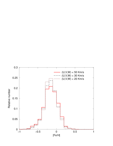
For this reason, we adopted the same AMR used for the full sample without kinematic selection. This is related to the debate over the existence of a distinct chemical history for disk and thick disk. It is well known that high velocity stars belong to more extended structures (thick disk and halo). Sandage (sand (1987)) and Casertano et al. (case (1990)), in particular, used kinematics to trace the thick disk population, but it is much less obvious that these stars reveal an age-metallicity relation that can be distinguished from that of the disk. Metallicity distributions of the thick disk and thin disk do not allow for an unequivocal separation. Some authors (see e.g. Gilmore et al. gilwy (1989), Bensby et al. ben (2005)) argue that the thick disk is a completely kinematically and chemically distinct Galactic zone; e.g. Bensby et al. (ben (2005)) determine a specific AMR, while a different conclusion is reached e.g. by Norris & Green (nor89 (1989)) and Norris & Ryan (nor91 (1991)), who argue that the thick disk is the high velocity dispersion tail of the old disk.

Figure 21 shows the recovered SFRs after 15 R-L restorations when the sample is kinematically selected. In particular, the result in the upper panel is found selecting objects with Galactic velocities within the velocity ellipse at $2\sigma$ for the thin disk. Result in the lower panel is found for objects with velocities within the velocity ellipse at $1\sigma$ for the thin disk.

The cut at $2\sigma$ excludes essentially all halo and thick disk objects. In this case (Fig. 21, upper panel), the recovered SFR is almost identical to the one without any selection. One explanation is that the contribution of thick disk and halo stars, for the period 1-8 Gyr, is minimal. This result confirms the general finding that the thick disk, if it exists, seems older than thin disk. For example Fuhrman (fuh (1998)) indicates 8 Gyr the thick disk age while Soubiran & Girard (soub (2005)) from 7 to 13 Gyr (with an average of $9.6\pm 0.3$ Gyr). In addition, the number density of local thick disk stars is a small fraction ($\sim 8\%$) of the thin disk stars. This result is confirmed by many works: Gilmore & Reid (gil83 (1983)) and Chen (chen (1997)) find 2%, Robin et al. (rob96 (1996)) find 6%, Soubiran et al. (soub03 (2003)) find 15%.

In contrast, by removing stars out of $1\sigma$ one should exclude:

• low velocity tails of halo and thick disk stars;

• disk stars whose orbits explore large scale heights (200-300 pc);

In this case, the recovered SFR (Fig. 21, lower panel) has a slightly lower peak at 3 Gyr, while the activity in the last 1.5 Gyr is increased. However, the variations are within the statistical uncertainties (between 1 and 2 $\sigma$ of acceptance) and the global trend is preserved.

Figure 21: Solid line: the recovered SFR using the full sample. Dashed line: the SFR recovered from stars with Galactic velocities within the velocity ellipse at $2\sigma$ (upper panel) and at $1\sigma$ (lower panel) the velocity ellipse of the thin disk.

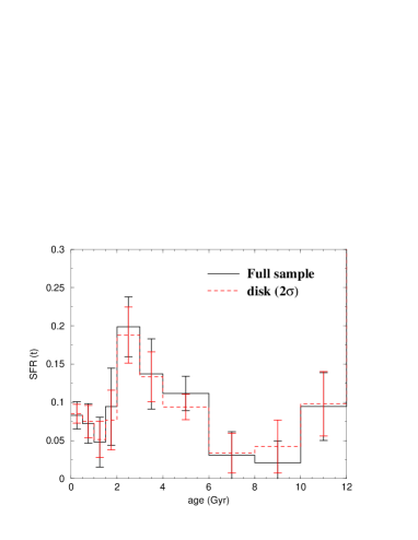
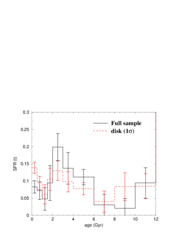
In conclusion, the recent SFR (last 6 Gyr) seems not to suffer of a significant dynamical diffusion. In this case, a correction for a possible disk depletion due to fast stars, does not really matter: within our level of acceptance, the recovered SFR is a genuine local SFR and not a mere local age distribution.

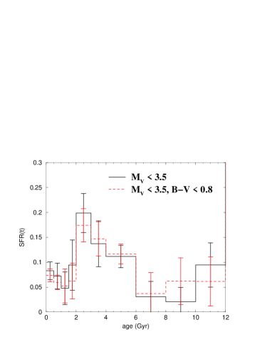
Because of the theoretical difficulties to reproduce the red clump stars (see the discussion in chapter 4), the analysis was repeated excluding all stars with $B-V>0.8$. In this case, because the excluded region involves stars of all ages, the recovered SFR (see Fig. 22) is slightly different at all ages (but still within the $1\,\sigma$ uncertainties), with a major effect around 10 Gyr.

Figure 22: The recovered SFR obtained from the full sample (solid line) and from a selection of stars with $B-V<0.8$ (dashed line).

8 Sensitivity to the adopted $(Z/X)_{\odot}$ value

Recent analysis of spectroscopical data using three dimensional hydrodynamic atmospheric models (see Asplund, Grevesse & Sauval aspl (2005) and references therein) have reduced the derived abundances of CNO and other heavy elements with respect to previous estimates (Grevesse & Sauval greve98 (1998), GS98). Thus the $Z/X$ solar value decreases from the GS98 value $(Z/X)_{\odot}=0.0230$ to $(Z/X)_{\odot}=0.0165$. GS98 already improved the mixture by GN93, widely adopted in the literature ($(Z/X)_{\odot}=0.0245$), mainly revising the CNO and Ne abundance and confirming the very good agreement between the new photospheric and meteoric results for iron. As already discussed our tracks are calculated for the GN93 solar mixture.

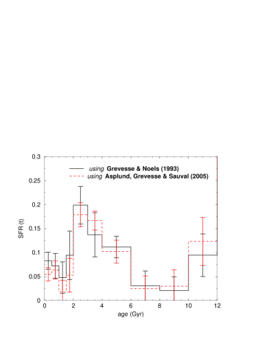
The change of the heavy element mixture can have two main effects: 1) the change of theoretical tracks at fixed metallicity (but this has been shown to be negligible; see Degl’Innocenti, Prada Moroni & Ricci ric (2006)); 2) the variation of the inferred metallicity from the observed $[Fe/H]$. This could be important for our purposes due to the adoption of the observational age-$[Fe/H]$ relation. Figure 23 compares the recovered SFR obtained using the Asplund, Grevesse & Sauval aspl (2005) or the GN93 solar mixture; the differences are within the statistical uncertainties.

Figure 23: Results for the recovered SFR obtained adopting the $Z/X$ solar value by Asplund, Grevesse & Sauval (aspl (2005)) (dashed line) and by GN93 (solid line).

9 Discussion and Prospects for Further Studies

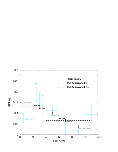
Our recovered SFR can be now compared with other recent published investigations. Bertelli & Nasi (bert (2001)), using a similar sample (Hipparcos stars within 50 pc and brighter than $M_{V}=4.5$) and a similar technique, found a local SFR that is independent by the chosen IMF, with the exception of low exponents (the value 1.3 is rejected). The figure 24 shows that our derived SFR is consistent with the ones by Bertelli & Nasi 2001. The small discrepancies could arise from the different inputs of the two models:

Figure 24: Our recovered SFR (dotted line) rebinned for comparison with Bertelli & Nasi 2001 (they used two functionally different assumptions for the star forming history: model a adopts a discontinuous change between two constant intervals of SFR; model b adopts a linearly increasing/decreasing SFR with a discontinuity in the slope at some time).

• The adopted evolutionary tracks: Bertelli & Nasi used the Padua stellar evolutionary tracks (Girardi et al. gira (1996)) which includes overshooting with an efficiency of about $0.12\,H_{P}$ in the mass range $1.0\,M_{\odot}<M<1.4\,M_{\odot}$ and $\approx 0.25\,H_{P}$ for higher masses. Our code implements the Pisa stellar tracks (Cariulo et al. car (2004), Castellani et al. cast03 (2003), Castellani, Degl’Innocenti & Marconi cast99a (1999)). Even if the red clump region is poorly reproduced by the Pisa stellar tracks, while the Padua tracks match better, we find (see Fig. 22) that clump and giant stars have a low impact on the recovered SFR for the last 6 Gyr.

• In the Bertelli & Nasi model the stars are uniformly distributed in the metallicity range $0.008\,<\,Z\,<\,0.03$. In contrast, we adopted the observational AMR by Nordström et al. (nord (2004)). Thus, their mean composition (solar) is metal richer than ours (using Grevesse & Noels greve (1993), the mean $[Fe/H]$ value $\sim-0.15$ corresponds to $Z\approx 0.012$).

• Bertelli and Nasi adopt between 30 and 70 percent of binaries (“decreasing from 70 percent for the more massive primaries to about 27 percent at the faint limit $M_{V}$=4.5”), while our models are without binaries. In the main sequence, the luminosity of a star depends on the mass, thus a binary system can mimic a different mass (and a different age); we already showed that reasonable binary fraction has no influence on the results (i.e. section 5.3), however the amount of binaries introduced by the authors could lead to some differences.

Schröder & Pagel (scho (2003)) also used Hipparcos stars within 100 pc and within 25 pc of the Galactic midplane. The SFR and the IMF are inferred by comparing the expected and observed numbers of stars in particular evolutionary phases (upper main sequence, clump, subgiants, etc.). These authors implemented the evolutionary tracks by Eggleton (egg (1973)) for solar metallicity. The presence of different chemical composition was taken into account by smearing the single metallicity CMD with a Gaussian spread. Their result is a local SFR that slowly increases towards recent times. The authors explain this as an effect of a dilution of the thin disk stars as they diffuse into larger scale heights by dynamical diffusion. In order to transform to a column-integrated SFR they adopted a dynamic diffusion timescale of about 6 Gyr. The final result is only slightly different from the local SFR (except the recent 1 Gyr, where the authors correct for a radial mixing). In practice, this result seems to confirm our finding that the dynamical diffusion of orbits has a low impact up to 6 Gyr before the present.

Within a Bayesian methodology, Hernandez et al. (her2 (2000)) used an inversion method on the Hipparcos stars brighter than $M_{V}=3.15$, deriving the local SFR for the last 3 Gyr. The implemented evolutionary tracks are the Padua isochrones (Girardi et al. gira (1996)) with $[Fe/H]=0$. In figure 25, it is shown our SFR against their findings for the last 3 Gyr (due to the lower temporal resolution of our SFR we needed to rebin the the higher time resolution of Hernandez et al. SFR).

Figure 25: Our recovered SFR (dotted line) compared with the Hernandez et al. (her2 (2000)) SFR (dashed line). Both the SFR are rebinned at 1 Gyr.

The two results are compatible, although our time resolution does not allow us to resolve the SFR behavior found by these authors (a cyclic pattern with a period of 0.5 Gyr). Considering that their sample is very similar ours, the differences in the result could be addressed to:

• Hernandez et al. (her2 (2000)) implemented a solar value ($[Fe/H]=0$) without spread, while we have adopted the Nordström et al. age metallicity relation;

• They used Padua isochrones (Girardi et al. gira (1996)), the same as Bertelli & Nasi (bert (2001));

• They implemented a power law IMF with exponent 2.7 (steeper than our value 2.35).

Moreover, because their technique is very different from our method, this agreement constitutes an independent verification of our method.

Vergely et al. (verg (2002)) used a similar inversion method. These authors determined simultaneously the star formation history, the AMR and the IMF from the Hipparcos stars brighter than $V=8$. The authors adopt a much larger sample (not magnitude limited) and the AMR is not constrained. Their result is a column SFR. The surprising feature is the similarity between their result (not local), see Fig. 26, and our SFR (local). In particular, their column-integrated SFR decreases with lookback time on a timescale of 4-5 Gyr, essentially the result we obtain.

Figure 26: Vergely et al. (verg (2002)) recovered SFR (heavy dot-dashed line) compared with our result (dotted line).

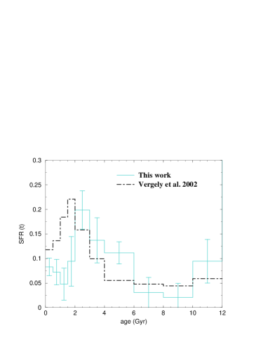
This supports our result and can mean:

• the local stellar population is not depleted in the past, but the derived SFR represents a genuinely lower activity;

• no significant dynamical diffusion has taken place on a time scale of 4-5 Gyr.

Rocha-Pinto et al. (roch (2000)) provided a SFR based on chromospheric emission ages for a sample of solar-like stars within 80 pc. Their result shows enhanced SFR episodes at 0-1 Gyr and 2-5 Gyr, that are approximately similar to our result, and at 7-9 Gyr (but it could be a spurious effect due to the low chromospheric emission for these ages). Also these authors find that the effect of dynamical orbit diffusion is not severe and does not affect the general trend of the SFR.

In conclusion, our result seems to represent a realistic SFR of the solar neighborhood. The recovered SFR is quite independent of the kinematical selections, suggesting that all the stellar generations (in the last 6 Gyr) are well represented and stars are not diffused in a larger volume. The SFR is consistent with other studies based on similar samples and different techniques. The result that our local SFR is close to the column SFR (Vergely et al. verg (2002)) seems to indicate that our result is not local and may be valid for the whole disk.

Having checked that dynamical diffusion has not been so efficient in the last 5-6 Gyr and the internal assumptions of the model (IMF, binaries, adopted solar mixture) have a low impact on the result, we can discuss the physical implication of our results.

The SFR obtained in the present work is concentrated in the recent 4 Gyr, that is a timescale longer than Galactic disk rotation ($<1$ Gyr). This result essentially rules out the possibility that this phenomenon is local, suggesting Galactic scale triggering event. It is difficult to explain our result if the Galactic disk is a “closed box” (see e.g. Van den Bergh van (1962), Schmidt schm (1963)): in this case the resulting SFR would be decreasing from the disk formation to the present (in opposition to our result), following the normal exhaustion of the gas content and an increased production of inert remnants. Even if the disk is periodically refilled with gas, our result is difficult to explain: the resulting SFR would be nearly constant in time (unless the infall is huge, but in this case the age-metallicity relation would change relative to observational evidence; e.g. Valle et al. valle (2005)).

Thus, the recovered SFR seems to indicate some kind of induced event, for example by the accretion of a satellite galaxy. However, the tracks left by a such an intruder should be recognized in the age-metallicity relation, while the survey of Nordström et al. (nord (2004)) shows practically no change in mean metallicity from 1 to 12 Gyr. An accretion should be evident from the analysis of the kinematical properties of stars in different age bins, but the methods to obtain stellar ages are still affected by large errors (see discussion in section 6.1).

Much larger surveys of stellar ages and metallicities as a function of galactocentric distance and kinematics are needed to test our hypothesis: comparing results from different regions of the disk could make clear if the recovered event is really a global event.

10 Conclusions

We have used a selection of the Hipparcos stars to recover the local SFR. The analysis is restricted to the stars within 80 pc and brighter than $M_{V}=3.5$. Numerical experiments with artificial CMDs show that, at these luminosities, neither the IMF nor the binary fraction are critical inputs, while the possibility to recover the SFR is strongly influenced by the adopted age-metallicity relation.

In particular, this result was checked assuming the observational AMR for the solar neighborhood by Nordström et al. (nord (2004)): the simulation with artificial CMDs indicate that most of the information about the underlying SFR is still recoverable. Finally, we applied the algorithm to real Hipparcos data. In contrast with artificial CMDs, the first problem was the presence of observational uncertainties (due to photometric and parallax errors). To take these uncertainties into account, we applied to the data the Richardson-Lucy technique as introduced in Cignoni & Shore (cign (2006)), cleaning the Hipparcos CMD from the observational errors. Then, assuming the observational AMR by Nordström et al. (nord (2004)), we have found the most probable SFR from our sample. The result indicates that the recent local SF history of the Galactic disk is increasing from the past to the present with some irregularities. The mean value increases very steeply from 6-7 Gyr ago up to 2 Gyr, in a way qualitatively similar to the findings of Vergely et al. (verg (2002)) and Bertelli & Nasi (bert (2001)). In particular, this result is is quite independent against kinematic selections, suggesting that:

1. The local contamination of halo and thick disk stars is negligible in the last 6 Gyr and/or these populations are older than 6 Gyr;

2. In the last 5-6 Gyr, all the stellar generations are well sampled; in other words, the recovered local SFR seems not to be biased by dynamical diffusion and the local volume is not “depleted” by old disk stars.

The timescale of the recovered SFR seems too long (larger than the dynamical timescale) to be attributed to local events: an accretion of a satellite galaxy is suspected.