Processing of turbulence-layer wind speed with Generalized SCIDAR through wavelet analysis

Abstract

We describe a new method involving wavelet transforms for deriving the wind velocity associated with atmospheric turbulence layers from Generalized SCIDAR measurements. The algorithm analyses the cross-correlation of a series of scintillation patterns separated by lapses of $\Delta t$, 2$\Delta t$, 3$\Delta t$, 4$\Delta t$ and 5$\Delta t$ using wavelet transforms. Wavelet analysis provides the position, direction and altitude of the different turbulence layers detected in each cross-correlation. The comparison and consistency of the turbulent layer displacements in consecutive cross-correlations allow the determination of their velocities and avoid misidentifications associated with noise and/or overlapping layers. To validate the algorithm, we have compared the velocity of turbulence layers derived on four nights with the wind vertical profile provided by balloon measurements. The software is fully automated and is able to analyse huge amounts of Generalized SCIDAR measurements.

1 Introduction

Adaptive optics in astronomy is a poweful technique that compensates for the distortions introduced by the atmosphere on the quality and resolution of images taken by ground-based telescopes. The excellent image quality requirements of the new generation of large and extremely large telescopes demands a proper knowledge of atmospheric turbulence in order to design efficient adaptive optics systems. Knowledge of the spatial and temporal behaviour of atmospheric turbulence at an astronomical site is crucial for optimizing the efficiency and operation of adaptive optics systems working with several deformable mirrors (multiconjugate adaptive optics). The SCIntillation Detection And Ranging technique (SCIDAR) is the most contrasted and efficient remote sensing technique for obtaining the optical vertical structure of atmospheric turbulence. The SCIDAR technique, its implementation and results have been extensively explained in several papers (Vernin & Roddier 1973; Rocca, Roddier & Vernin 1974; Fuchs, Tallon & Vernin 1994; Avila, Vernin & Masciadri 1997; Kluckers et al. 1998; Johnston et al. 2002).

In the last few years, several campaigns for atmospheric turbulence characterization have been carried out at different astronomical sites, many of them using the generalized SCIDAR (G-SCIDAR hereafter) technique (Avila, Vernin & Cuevas 1998; Avila et al. 2003; Kluckers et al. 1998; Vernin et al. 2000; McKenna et al. 2003; Fuensalida et al. 2004a,b; Avila et al. 2006). The refractive index structure constant profiles, $C_{N}^{2}$(h), are derived from SCIDAR observations through automatic programs using inversion methods (Vernin 1992; Kluckers et al. 1998; Prieur, Daigne & Avila 2001; Johnston et al. 2002). The velocities of the turbulent layers are obtained through interactive programs (Kluckers et al. 1998; Avila et al. 2001, 2003; Vernin et al. 2000) based on the CLEAN method, (Prieur et al. 2001) and the first iterative and potentially automated algorithm also based on the CLEAN procedure has been recently published (Prieur et al. 2004). We present here an alternative method for deriving the wind velocity of turbulence layers from G-SCIDAR measurements based on wavelet analysis. We have developed fully automatic software that is very suitable for analysing huge amounts of SCIDAR data based on this new method.

In Section §2 we briefly describe the G-SCIDAR technique. A brief introduction to wavelet analysis applied to the problem of determining wind turbulence profiles is presented in Section §3.1. The input data for the algorithm are shown in Section §3.2 and we describe the algorithm in Section §4. The velocity of turbulence layers derived from our wavelet-based method are compared to wind vertical profiles measured using balloons (Section 5). In this paper we present only the developed wavelet-based method and results derived from a few G-SCIDAR observations compared to balloon measurements to test the proposed algorithm. We are already preparing a paper with the statistical results of the wind velocity of turbulent layers above the Canary Islands astronomical observatories from long-term SCIDAR measurements.

2 Brief description of the G-SCIDAR technique

Classical techniques (Vernin & Roddier 1973; Rocca, Roddier & Vernin 1974) and G-SCIDAR (Fuchs, Tallon & Vernin 1994; Avila, Vernin & Masciadri 1997; Kluckers et al. 1998) analyse the scintillation patterns produced at the telescope pupil by the light coming from the stars in a binary system. Turbulence profiles as a function of height, $C_{N}^{2}(h)$, are derived through the inversion of the average normalized autocovariance of a large number of scintillation patterns (see Fuchs et al. 1994 and references therein for a detailed description of G-SCIDAR theory).

Figure 1: (a) Principle of the SCIDAR technique considering a single turbulence layer. $\delta$ corresponds to the angular separation between the stars in the binary system. h is the altitude of the turbulence layer over the observation plane. D corresponds to the distance between the lateral peaks of the normalized autocorrelation. (b) The average normalized autocorrelation of a series of scintillation patterns at the telescope pupil produced by a single turbulent layer on the light coming from a binary star. (c) The principle of G-SCIDAR considering multiple turbulence layers. $h_{1}$ and $h_{2}$ indicate the altitude of two turbulence layer over the analysis plane. The obs line represents observatory level. $h_{a}$ corresponds to the position of the analysis plane below observatory level. $D_{1}$, $D_{2}$ and $D_{a}$ indicate the distance between the lateral peaks of the normalized autocorrelation produced for the different turbulence layers considered.

Figure 2: Maps in this figure are only simulations to illustrate the problem and do not correspond to real data.(a) Simulation of the average normalized autocorrelation of a series of scintillation patterns at the telescope pupil produced by three turbulent layers on the light coming from a binary star. $D_{1}$, $D_{2}$ and $D_{a}$ indicate the distance between the lateral peaks of the normalized autocorrelation produced for the different turbulence layers considered as in Figure 1c. (b) Simulated cross-correlation of scintillation images separated by a lapse $\Delta t$. (c) Simulated cross-correlation of scintillation images separated by a lapse 2$\Delta t$. (d) Simulated cross-correlation of scintillation images separated by a lapse 3$\Delta t$. (e) Simulated cross-correlation of scintillation images separated by a lapse 4$\Delta t$. (f) Simulated cross-correlation of scintillation images separated by a lapse 5$\Delta t$. $V_{1}$, and $V_{2}$ are the wind speeds of two turbulence layers over the observing site, while $V_{a1}$ corresponds to the speed of a turbulent layer close to the altitude of the observing site.

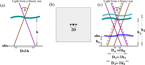
While classical SCIDAR was insensitive to turbulence at low altitudes, with G-SCIDAR low altitude atmospheric turbulence can be separated from the dome contribution (Fuchs, Tallon & Vernin 1994). In G-SCIDAR, the plane of observations lies a few kilometres below the telescope pupil, while the telescope pupil is the analysis plane in the classical SCIDAR.

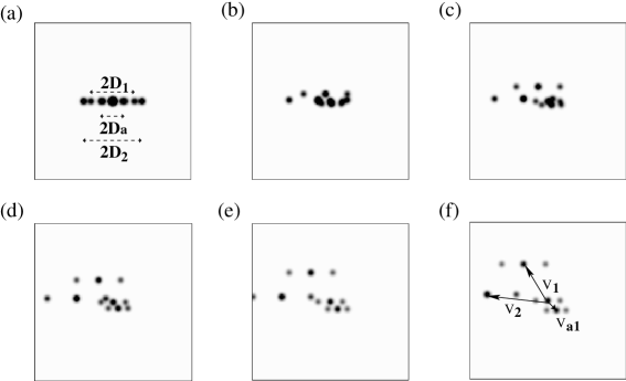
For a single turbulent layer at an altitude h above the ground (Fig. 1a), the average normalized autocorrelation of several scintillation patterns from SCIDAR measurements of a binary system will result in a frame with three peaks (Fig. 1b). The distance D between the lateral and central peaks is related to the angular separation ($\delta$) of the two stars forming the binary system and the altitude of the turbulence layer (h), as is illustrated in Figure 1a. When the atmosphere presents several turbulent layers (Fig. 1c) the result from the analysis of G-SCIDAR measurements will be a frame with several lateral peaks (Fig. 2a). In this map, the central peak includes the contribution of the different turbulent layers. Lateral peaks equidistant from the central peak indicate the intensity and altitude of a particular turbulent layer. $C_{N}^{2}(h)$ is basically derived through the inversion of the cut connecting the peaks (Vernin 1992; Kluckers et al. 1998; Prieur, Daigne & Avila 2001; Johnston et al. 2002).

Wind velocity of turbulence layers can be derived from the average normalized cross-correlation of a series of scintillation patterns relative to a reference pattern (Avila et al. 2001). If we consider a single turbulent layer with a wind velocity $\mathbf{\stackrel{{\scriptstyle\rightarrow}}{{V}}}$ , the average normalized cross-correlation of two scintillation patterns taken at times separated by $\Delta t$ will result in a map with a triplet placed at $\mathbf{\stackrel{{\scriptstyle\rightarrow}}{{V}}}$$\Delta t$ from the central peak of the corresponding average normalized autocorrelation. In the most realistic case of several turbulent layers moving at different wind velocities, the resulting frame will show several triplets located at different positions according to the wind vector of each layer (Fig. 2b). When we take frames separated by $n\Delta t$, the triplets will placed at $n$$\mathbf{\stackrel{{\scriptstyle\rightarrow}}{{V}}}$$\Delta t$ from the central peak (0,0). Figures 3c–f show the average normalized cross-correlation of two scintillation patterns taken at 2$\Delta t$, 3$\Delta t$, 4$\Delta t$ and 5$\Delta t$, respectively. In these simulated cross-correlations, layers are well resolved for scintillation patterns taken after 3$\Delta t$, which is not far from the real case. The altitude of the different turbulent layers is determined by the distance of the lateral to the central peak of each triplet, as in the autocorrelation. The distance and relative position of triplets with respect to the centre of the frame determine the wind speed of each turbulence layer. Information on the velocity of relatively faint turbulent layers can eventually be missed in the cross-correlation owing to temporal decorrelation of the scintillation and/or eventual fluctuations of $\mathbf{\stackrel{{\scriptstyle\rightarrow}}{{V}}}$ during the integration time (Avila et al. 2001).

It is important to note that the SCIDAR technique provides wind speed measurements only where a turbulence layer is detected.

3 Wavelet-based algorithm for deriving turbulence layer wind speed

3.1 Wavelet-based transform application

Wavelets are mathematical functions that decompose data into different frequency components allowing each component to be studied separately. The basic idea behind wavelet analysis is to take a mother wavelet ($M(X)$), translate and dilate it ($M_{a,b}(X)$), integrate it product with the signal $(F(X))$ and study the coefficients in wavelet space, spanned by translation b and dilation a. The set of functions $M_{a,b}(X)$ are given by

$$\centering M_{a,b}(X)=\frac{1}{a^{1/2}}M(\frac{X-b}{a}),\@add@centering$$ (1)

where a and b are real, a being greater than 0. Wavelet analysis is based on the integration of the $F(X)$ products with the set of functions $M_{a,b}(X)$ :

$$T_{M}({\it b,a})=\frac{1}{a^{1/2}}\int M^{*}(\frac{X-b}{a})F(X)dX,$$ (2)

where b is the translation parameter and corresponds to position or time when the data is spatial or temporal, respectively. The dilation parameter a corresponds to scale length or temporal period. M^∗ indicates the complex conjugate of M. The wavelet transform (Equation 2) expands a one-dimesional function, $F(X)$, into a two-dimensional parameter space, the wavelet space (b, a) giving a local measure of the relative amplitude of activity at scale a and at space/time b. Wavelet analysis has been applied in a wide variety of scientific fields, including atmospheric sciences, engineering, financial analysis, geophysics, image analysis, medical science, turbulence, etc. A practical introduction and description of wavelet analysis can be found, for example, in Torrence & Compo (1998) and Mayers, Kelly & O’Brien (1993).

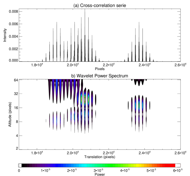
In order to derive the velocity of the turbulence layers from SCIDAR observations using wavelets, we have transformed each cross-correlation ($C(X,Y)$) into a one-dimensional function ($F(X^{\prime})$) placing the different lines $Y$ consecutively (see Fig. 3). Therefore, $F(X^{\prime})$ is a one-dimensional function of $X\times Y$ elements where each set of $X$ elements corresponds to a $Y$ line in the $C(X,Y)$. Hence, $F(X^{\prime})$ is a function in spatial space, where each element corresponds to a well-define position in the $C(X,Y)$. In the wavelet space, the translation parameter b can be identified with the position $X^{\prime}$ and hence to the position in the cross-correlation $C(X,Y)$. Therefore, b gives information about wind speed (velocity and direction). The dilation parameter a is related to the distance between the lateral peaks to the central peak of each turbulent layer. Hence, a can be identified to the altitude of the different turbulent layers.

Figure 3: Transformation of each cross-correlation $C(X,Y)$ derived from SCIDAR observations into a one-dimensional function $F(X^{\prime})$ to apply the 1D wavelet algorithm.

For the analysis of $F(X^{\prime})$, we have selected a commonly used mother wavelet, the Morlet function. The Morlet wavelet consists of a plane wave modulated by a Gaussian,

$$M(x)\approx e^{i\omega_{0}x}e^{-x^{2}/2},$$ (3)

where $\omega_{0}$ is a non-dimensional scale length (space) or frequency (time) that we take as 6 to satisfy the condition that the wavelet function have zero mean and be located in both space/time and scale/frequency space (Farge 1992). Considering the form of the Morlet wavelet, equation (2) is only the convolution of the signal, F(X’) with a set of Morlet functions. The result of the convolution of $F(X^{\prime})$ with Morlet wavelets (a sequence of translated and dilated Morlet functions) is a 2D function in wavelet space (b,a) with the brightest peaks indicating the wind speed (b component) and the turbulent layer altitude (a component). Figure 4 shows an example of the 2D function in the wavelet space derived from the convolution of the simulated cross-correlation frame in Figure 2d transformed to a 1D function (as in Figure 3) and a series of Morlet functions. The wavelet power spectrum presents several bright knots, the brighter ones corresponding to each of the turbulent layers. Fainter knots placed at the same translation position as the brighter ones correspond to harmonic frequencies (see also Fig. 5). In Section §3.2 we explain the way we select or reject a peak in the wavelet power spectrum to determine the wind speed of the turbulence layers.

Figure 4: (a) The 1D cross-correlation series derived from the cross-correlation of Fig. 2d, as explained in Figure 3. (b) The wavelet power spectrum derived through the convolution of the 1D cross-correlation series with a set of Morlet wavelets (a dilated and translated Morlet function). The horizontal axis of this plot corresponds to a well-defined position in the cross-correlation, and the vertical axis indicates the separation of the lateral peaks of each detected triplet in the cross-correlation. The brightest peaks in this 2D map corresponds to position of the central peak of each triplet.

3.2 Wavelet-based algorithm for wind velocity measurements

The algorithm proposed in this paper is based on wavelet transforms. As we explained in Section §3.1, the peaks of the wavelet power spectrum derived from the convolution of the 1D cross-correlation with a set of Morlet functions provide information about the location of the triplets in the input data, as well as the separation of the lateral peaks. The basic idea of the method is to extract the velocity of the turbulent layers by the consistencies of its displacements in consecutive wavelet power spectra obtained from the cross-correlation of scintillation patterns taken at intervals $\Delta t$, 2$\Delta t$, 3$\Delta t$, 4$\Delta t$ and 5$\Delta t$. As we have five cross-correlations, we have five different 1D cross-correlation inputs for the wavelet analysis. Therefore, we get five wavelet power spectra. The algorithm has already been tested with simulated data (García-Lorenzo & Fuensalida 2006).

The first step in the processing of the data is noise filtering in the cross-correlation frames. Different sources contribute to the noisy background: noise from the detector, electronic noise, and noise associated with the finite dimensions of the images. We first identify the pixels in the cross-correlations (and auto-correlation) with values smaller than zero and change their value to zero. From the autocorrelation, we eliminate the central pixels, where the triplets corresponding to the turbulence profiles appear (Fig. 2a), and we calculate the background median of the pixels larger than zero (BM hereafter) and their standard deviation (ST hereafter). BM and ST are taken as references for the noise filter. The noisy background of the cross-correlations is evaluated as the pixels in these maps with values smaller than BM plus a factor of ST. A default value of 3 is adopted for the automatic processing of the data, although this factor can also be selected by the user when starting the analysis of the data with the developed software. If a factor two is selected, we call a sigma2 filter for the analysis. For a factor four, we call a sigma4 filter. Those pixels satisfying the noise filtering conditions are taken as zero, and only pixels with values larger than the noise filter conditions are considered as real signal.

The wavelet algorithm starts analysing the cross-correlation corresponding to 5$\Delta t$, which we refer to hereafter as cc5. The peaks located in the wavelet power spectrum are caracterized by two coordinates. The horizontal coordinate gives information about the location of the triplet in cc5 (the velocity vector), and the vertical coordinate corresponds to the separation of the lateral peaks of the triplets (the height of the turbulent layer). In order to discard any harmonic frequency or any peak associated with noise, we compare the derived coordinates with 5cc. For each peak detected in the wavelet power spectrum, we translate its coordinates to cc5 and check that, at the calculated position, there exists a triplet with the lateral peaks separated by as much as the vertical coordinate indicates. If the validation is positive, the coordinates of that peak are saved in an intermediate file. Those peaks of the wavelet power spectrum with a negative validation are considered as harmonics or noise and are deleted from the rest of the analysis. Figure 5 presents an outline of the procedure over the cross-correlation shown in Figure 2d. Sometimes, a few peaks that are not associated with any real triplet but with noise are not eliminated in this first step of the algorithm.

Figure 5: Schematic view of the procedure for validating triplets located in the wavelet power spectrum from the wavelet analysis of a cross-correlation. In the top left panel, we present the input data, the cross-correlation at $n\Delta t$. The top-right panel corresponds to the wavelet power spectrum derived from the wavelet analysis. The filled circles mark the selected points to explain the method for validating the triplets. The bottom-right panel indicates the points giving a positive validation. The file with the validated triplets, their corresponding position in the cross-correlation and the separation between the lateral peaks is shown in the bottom-left panel.

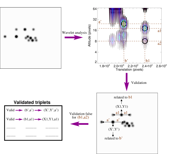
We follow the same procedure for the cross-correlations at 4$\Delta t$ (cc4 hereafter) and 3$\Delta t$ (cc3 hereafter). Once we have proccesed cc5, cc4, and cc3, we translate to 3$\Delta t$ the validated triplets for each cross-correlation using the relationship: $Velocity=Space/Time$. In this way, any triplet located at coordinates ($X_{n}$,$Y_{n}$) at $n\Delta t$ will be placed at the position:

$$(X_{3},Y_{3})=(X_{n},Y_{n})\frac{3\Delta t}{n\Delta t}.$$ (4)

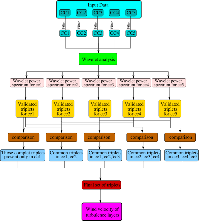
We then compare the three sets of points at the same temporal position 3$\Delta t$. Those points at the same coordinates and showing the same distance between lateral peaks are identified as true triplets. To compare coordinates, we allow an uncertainty equal to the full width half maximum of the central peak of the triplets. It is clear that any triplet in cc5 must be at cc4 and cc3, although triplets present at cc4 and/or cc3 corresponding to faster layers could be missing in cc5. We continue the analysis in the same way, now comparing cc4, cc3 and the cross-correlation corresponding to 2$\Delta t$ (hereafter cc2). Triplets at cc4 must be in cc3 and cc2, but the triplet in cc3 and cc2 could be absent in cc4. We compare cc3, cc2 and the cross-correlation at $\Delta t$ (hereafter cc1), and finally, we compare the results for cc2 and cc1. The triplet in cc2 must be in cc1, although these tend to be blended into one another. The coordinates of the final validated triplets are transformed to the velocity and altitude using the determined parameters of the observational setup ($\Delta t$,the conjugated plane, observatory altitude, etc.). To summarize, Figure 6 shows a schematic view of the algorithm. We are able to identify high velocity turbulent layers if the central and one of the lateral peaks are present in cc1 at least. Only those triplets associated with turbulence layers moving as fast as they have disappeared in cc1 are undetected in our procedure. These kinds of layers should be (a) very fast and in low-altitude or (b) high-altitude layers of moderate velocity. For our system (see section §4.1 for details), in a configuration with the conjugate plane at four kilometres and a binary star with an angular separation of 9.6 arcsec, a low-altitude turbulence layer moving faster than 45 m/s or a high altitude layer (over 18 000 m) moving faster than 29 m/s will be lost from the analysis depending on the direction. Low altitude layers faster than 45 m/s are associated with bad weather conditions, when the telescope is closed due to wind limitions on telescope operation. For the second case, when a high-altitude layer is moving at a moderate velocity the proposed algorithm will miss the layer. Indeed, the instrument configuration (see Section §4.1) will miss the velocity information on such turbulence layer and only increasing the sample frequency will retain such information. High altitude turbulence layers moving faster than 30 m/s have been already reported on San Pedro Mártir. However, the statistical study of wind vertical profiles at different astronomical sites (García-Lorenzo et al. 2005) indicates that such fast winds do not occur very often at high altitudes. Moreover, the turbulence above the Canary Islands observatories tend to be concentrated in low-altitude layers (Fuensalida et al. 2004). Therefore, the second case should not be a habitual situation in our data.

A few programs have been already developed for the determination of wind profiles from G-SCIDAR observations (Kluckers et al. 1998; Avila et al. 2001, 2003; Vernin et al. 2000; Prieur et al. 2004). The advantage of our procedure is not only the new algorithm, but also that we make use of five cross-correlations instead of two, as with previous programs and therefore have a higher resolving capacity of slow layers. The processing of more maps represents a higher computer dedication, but it minimize several common problems. The detection of dome seeing (layers with $V=0$ in the cross-correlations) is easier when using five cross-correlations, which is an advantage of the developed procedure over previous works (Kluckers et al. 1998; Avila et al. 2001, 2003; Vernin et al. 2000; Prieur et al. 2004). For example, in Fig. 3, the layer corresponding to dome seeing (the central triplet with $V=0$) is blended with other turbulence layers in the cross-correlation at $\Delta t$ (Fig. 2b) and 2$\Delta t$ (Fig. 2c), while it appears resolved from the cross-correlation at 3$\Delta t$ (Fig. 2d). Therefore, for cross-correlation of scintillation patterns with lapses of 5$\Delta t$, only low-altitude turbulence layers with velocities smaller than twice the velocity resolution of the system can be confused with dome seeing.

In Section §4 we present some examples and explanations to illustrate the automatic program.

Figure 6: Schematic view of the algorithm for computing wind velocities of turbulence layers for SCIDAR observations (see Section §3.2).

4 Wind profile results from the wavelet-based algorithm

In this section, we present a few examples to illustrate the data processing with the proposed algorithm on real G-SCIDAR observations. We compare the derived velocity of the turbulence layers with the vertical wind profile measured with balloons.

4.1 The Data

The data analysed in this paper were obtained on 2003 July 23, August 5–6 and August 31 at the Observatorio del Teide (OT) on the island of Tenerife (Spain). The 1.5 m Carlos Sánchez Telescope (1.5m-TCS) was used in combination with the G-SCIDAR instrument developed at the Instituto de Astrofísica de Canarias (IAC). Each detector pixel covers a square of side 2.81 cm on the 1.5m-TCS pupil. We used 1000 images of scintillation patterns to derive the average normalized autocovariance and five frames that are measurements of the 2D spatiotemporal cross-correlation functions separated by a lapse of $\Delta t$ equal to 26 ms, 52 ms, 78 ms, 104 ms and 130 ms. These sets of frames are similar to those maps in Fig. 2 and they constitute the experimental data input to the wavelet-based algorithm in order to determine the wind velocity of the turbulence layers.

For comparison and validation of wind speed derived from the wavelet-based algorithm, we have used wind vertical profiles measurements from the closest radiosonde station located $\sim$13 km from the OT. The Centro Meteorológico Territorial de Canarias Occidental of the Spanish Instituto Nacional de Meteorología (INM: http://www.inm.es) operates this radiosonde station, which is part of the NOAA network (station 60018). Radiosondes are launched twice daily (at 12Z and 00Z) from an altitude of 105 m and reaches an altitude of around 30 km. We have selected the radiosonde data obtained at 00Z for the nights of our SCIDAR observations.

4.2 Examples of Processing

The developed software is able to evaluate the wind velocity of turbulent layers for the data of a full night or only the wind velocity associate with a particular G-SCIDAR measurement. The first example of processing corresponds to the latter case. We have selected a sigma4 filter for the noise filtering (see Section §3.2). Figure 7 shows the autocorrelation (Fig. 7a) and the five cross-correlations (Fig. 7b, 7c, 7d, 7e and 7f) frames corresponding to that particular measurement before (Fig. 7(1)) and after (Fig. 7(2)) the noise sigma4 filter was applied.

Figure 7: (a) The average normalized autocorrelation of 1000 scintillation patterns observed at the TCS pupil produced by turbulent layers on the light coming from the binary star BS 7948 on the night of August 31 at around 23 UT. (b) Cross-correlation of the same series of scintillation images as (a) but separated by a lapse of $\Delta t$ = 26 ms. (c) Cross-correlation of the same series of scintillation images as (a) but separated by a lapse of 2$\Delta t$ = 52 ms. (d) Cross-correlation of the same series of scintillation images as (a) but separated by a lapse of 3$\Delta t$ = 78 ms. (e) Cross-correlation of the same series of scintillation images as (a) but separated by a lapse of 4$\Delta t$ = 104 ms. (f) Cross-correlation of the same series of scintillation images as (a) but separated by a lapse of 5$\Delta t$ = 130 ms. The lefthand plots (1) correspond to drawn frames and the righthand plots (2) are maps after the noise filter sigma4 were applied.

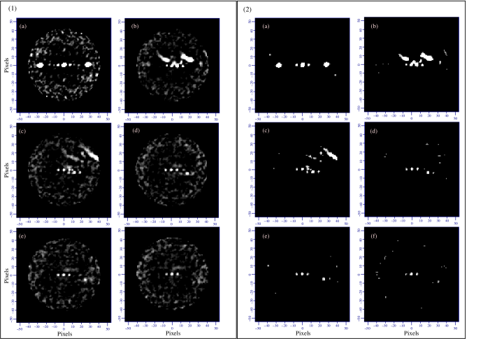
From the wavelet analysis of each cross-correlation after noise filtering, we obtain a wavelet spectrum and we analyse the peaks of these wavelet spectra as explained in Section §3.2. For comparison, Figure 8 shows the identified triplets in the wavelet power spectrum corresponding to each cross-correlation function analysed on the same scale as the maps in Figure 7. Each point in Figure 8 corresponds to the position of the central peak of each identified triplet. Figure 8f shows the final triplets selected from the comparison of the validated triplets in each cross-correlation. Scale in Figure 8f is larger than in the other plots in Figure 8 in order to include those triplets that only appears in cc1 and cc2. Bear in mind that the comparison is made at 3$\Delta t$ (see Section 3.2). From the analysis of this particular G-SCIDAR measurement we have detected three different turbulence layers moving at different velocities. The first identified turbulence layer is the dome seeing and corresponds to the points around the origin of coordinates in Figures 7 and 8 with velocity equal to zero (the same position at the auto-correlation and the five cross-correlations). The second turbulence layer is moving from the centre to the bottom right of the frames with a relative slow velocity. It corresponds to a low-altitude turbulent layer close to or at observatory level. This second layer is located at around the pixel (20,$-7$) at 3$\Delta t$ (Figure 8). The third turbulence layer identified is moving quickly from the centre to the upper right of the frames. This third layer is composed of several layers apparently at similar altitudes but moving with different velocities. Actually, it seems to correspond to a velocity-stratificated layer formed by thinner turbulence layers situated at slightly different altitudes. The wavelet algorithm allows us to separate the stratification if the velocity difference between the thinner layers is larger than the velocity and altitude resolution of the experimental setup.

Figure 8: Location of triplets identified in the wavelet spectrum of (a) cc1 ; (b) cc2; (c) cc3; (d) cc4; (e) cc5. (f) Location of the validated triplets after the comparison of identified triplets for each particular wavelet spectrum (as explained in Section §3.2). Please note that axis scale is much larger in this plot to include all the identified layers at 3$\Delta t$.

The coordinates of the final validated triplets are transformed to velocity and altitude using the parameters of the observational setup ($\Delta t$,the conjugated plane, observatory altitude, binary star angular separation, etc.). The velocity and altitude resolution of the proposed algorithm is better than the current resolution provided by the inversion algorithm for the turbulence profile. For this reason, we bin the resolution of the velocity profile to the turbulence intensity profile. Such better resolution can be used to obtain the contribution of each turbulent layer detected in the cross-correlation to the $C_{N}^{2}$ profile following, for example, the approach by Avila et al. (2001). We are developing an improved wavelet-based algorithm to determine simultaneously the velocity and $C_{N}^{2}$ of individual turbulent layers in order to increase the resolution on the determination of the $C_{N}^{2}$ profile. For this subject, we impose the condition that the sum of $C_{N}^{2}$ associated with individual layers should be equal to the $C_{N}^{2}$ profile derive from the autocorrelation. However, this issue is complex to tackle because of the presence of harmonics in the wavelet spectrum and the temporal decorrelation of scintillation (Avila et al. 2001). In this paper, we concentrate on the determination of velocities of turbulent layers and we have left the calculation of their associated $C_{N}^{2}$ values for a new and improve version of the current software.

It is important to note that the velocity vector derived from G-SCIDAR measurements is in fact the projection of the actual velocity vector of the turbulence layer on the plane perpendicular to the observing direction (e.g. Avila et al. 2001). Such projection affects both the module and direction in different ways. The appendix A presents the expresions for the errors when deriving the velocity vector from G-SCIDAR observations as a function of the actual wind vector of the turbulence layer.

The developed software does not correct for projection effects on the determination of the wind direction because such projections are small as the observations are carried out at zenith angles smaller than 30^∘. In particular, errors smaller than four degrees are archived when deriving the wind direction (see Appendix A). This is more than acceptable taking into account that the wind orientation is not important when deriving the relevant temporal parameters for adaptive optics. The developed software includes the correction of projection effects when determining the wind module. The percent errors associated to the wind module depend on the wind direction of each turbulence layer respect to the azimuth of the observation. For zenith angles of 30^∘, such errors could be as larger as 14% when the actual velocity vector of the turbulence layer is on the direction of the azimuth (see Appendix A).

Figure 9 shows the derived turbulence profile and wind velocity of the particular G-SCIDAR measurement analysed in detail in this section.

Figure 9: (a) Vertical turbulence profile ($C_{N}^{2}$); (b) wind modulus of turbulence layers derived from the wavelet-based algorithm; (c) wind direction (in degrees) for the motion of turbulence layers derived from the wavelet-based algorithm

4.3 Comparison of results with balloon measurements

In order to validate results from the wavelet-based algorithm to determine the velocity of turbulence layers, we have used balloon measurements from the NOAA station 60018 (see Section §4.1). We have obtained an average $C_{N}^{2}(h)$ and wind profiles from the individual vertical profiles obtained approximately during the corresponding balloon ascent. Figure 10 shows the comparison of both wind measurements, indicating a remarkable correspondence between the SCIDAR and balloon measurements. To calculate the wind direction measured with G-SCIDAR we have used the position angle in the sky of the binary star observed to derived these profiles.

Figure 10: Wind vertical profiles (left) and the simulataneous vertical turbulence profile ($C_{N}^{2}$) for four nights (dates are indicated at the top of each plot). Error bars only indicates the standard deviation of the G-SCIDAR measurements (around 130 individual profiles) during the balloon ascent. The solid line in the left plot corresponds to wind speed measurements with radiosondes launched 13 km away from the Observatory and close to sea level. Filled dots are the derived velocities for turbulence layers from the G-SCIDAR measurements during the corresponding balloon ascent. The right panel of each plot shows the average (solid line) and median (dotted line) of the $C_{N}^{2}$ measurements derived from G-SCIDAR observations during the corresponding balloon ascent. The horizontal axis represents the $C{{}_{N}^{2}}$ on a logarithmic scale. The vertical axis corresponds to the altitude above sea level. The horizontal dashed line indicates the Observatory altitude (2400 m). Dome seeing has been removed from the profiles using a procedure based on the properties of the parity of functions (Fuensalida, García-Lorenzo & Hoegemann 2006).

In general, the altitude of turbulence layers in the average $C_{N}^{2}$ profile appears in regions where the balloon wind data present strong vertical gradients. This is the case for three of the four example nights (030723, 030805 and 030831). This is in good agreement with the idea that wind gradients break the stable stratification producing hydrodynamical instabilities and generating dynamical turbulence, which leads to the formation of turbulence layers in the presence of a potential temperature gradient (Coulman et al. 1995). The turbulence profile observed for the night 030806 presents turbulence layers associated with smooth gradients in the wind vertical profile (in modulus or direction) which might not be in concordance with the accepted scenario. We also identify strong vertical gradients in the vertical wind profiles that are not associated with any turbulence layer (night 030805 at around 10 and 15 km). However, we lack temperature gradient information to analyse those situations properly.

5 Conclusions

Monitoring programmes for atmospheric turbulence characterization are already in progress at several astronomical sites. Such characterization will allow us to improve current adaptive optic systems to compensate for the effects of turbulence on the light from astronomical objects. The development of powerful mathematical procedures and efficient software to treat turbulence data in real time will allow us to develop “active” adaptive optic systems. By “active” we mean an adaptive optic system using information on the turbulence structure in real time and with the capacity of fitting its parameters to the actual turbulence conditions.

We have presented a new automatic method for deriving the wind speed of turbulence layers from G-SCIDAR observations. The developed algorithm have a higher capacity of resolving slow turbulence layers than previous programs because we make used of five cross-correlation. Comparison of wind vertical profiles from G-SCIDAR and balloon measurements demonstrates the effectiveness of the propose algorithm. We illustrate the new algorithm with the results obtained for four nights of G-SCIDAR observations at the Observatorio del Teide on the island of Tenerife (Spain). The algorithm allows us to process a huge amount of G-SCIDAR data without human intervention. The developed software takes into account the effect of the projection of the actual velocity vector of turbulence layers on the observing direction when determining the wind module. The calculation of some important parameters for adaptive optics, such as the coherence time, can be strongly affected when such effect is not considered.

6 APPENDIX A:
Projection effects on the determination of the velocity vector of turbulence layers from G-SCIDAR observations.

The velocity derived from Generalized SCIDAR (G-SCIDAR hereafter) observations is in fact the projection of the layer velocity vector on a plane perpendicular to the observing direction. In this appendix, we calculate the mathematical expression for the error in the determination of the wind direction from G-SCIDAR due to such projection and assuming turbulence layer moving horizontally..

Let $XYZ$ be a three-dimensional coordinate system. The axes are depicted in a world-coordinates orientation with the $Z$-axis pointing up. For an astronomical site, the $Z$-axis represents the zenith direction.

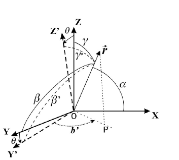
If we are observing a particular source at a Zenithal distance $\theta$, we can define a second three-dimensional coordinate system, $X^{\prime}Y^{\prime}Z^{\prime}$. Such a coordinate system can be selected as a coordinate system rotated about the $X$-axis; that is, $X^{\prime}Y^{\prime}Z^{\prime}\equiv XY^{\prime}Z^{\prime}$. In this way, the $Z^{\prime}$-axis represents the observing direction, so that, the $Z^{\prime}$-axis forms an angle $\theta$ with the $Z$-axis, and the $Y^{\prime}$-axis corresponds to the azimuth direction of the observation. Figure 11 shows the $XYZ$ and $XY^{\prime}Z^{\prime}$ coordinate systems.

Let (l_y, m_y, n_y) and (l_z, m_z, n_z) be the direction cosines of the $Y^{\prime}$ and $Z^{\prime}$ axis, respectively, in the $XY^{\prime}Z^{\prime}$ system expressed in function of $X$, $Y$, and $Z$ in the $XYZ$-system. Then,

Figure 11: A view of the coordinate systems $XYZ$ and $XY^{\prime}Z^{\prime}$.

$$y^{\prime}=l_{y}x+m_{y}y+n_{y}z\hskip 28.45274pt\Longrightarrow\hskip 28.45274pty^{\prime}=\cos\theta y-\sin\theta z$$ (5)

$$z^{\prime}=l_{z}x+m_{z}y+n_{z}z\hskip 28.45274pt\Longrightarrow\hskip 28.45274ptz^{\prime}=\sin\theta y+\cos\theta z$$ (6)

The direction of a vector $\mathbf{\stackrel{{\scriptstyle\rightarrow}}{{r}}}$ is determined by its direction cosines, given by (cos $\alpha$, cos $\beta$, cos $\gamma$) in the $XYZ$-system, and (cos $\alpha$, cos $\beta$’, cos $\gamma$’) in the $XY^{\prime}Z^{\prime}$-system (see Fig. 11:

$$x_{r}=|\mathbf{\stackrel{{\scriptstyle\rightarrow}}{{r}}}|\cos\alpha;\hskip 22.76228pty_{r}=|\mathbf{\stackrel{{\scriptstyle\rightarrow}}{{r}}}|\cos\beta;\hskip 22.76228ptz_{r}=|\mathbf{\stackrel{{\scriptstyle\rightarrow}}{{r}}}|\cos\gamma$$ (7)

$$x^{\prime}=|\mathbf{\stackrel{{\scriptstyle\rightarrow}}{{r}}}|\cos\alpha^{\prime};\hskip 19.91684pty^{\prime}=|\mathbf{\stackrel{{\scriptstyle\rightarrow}}{{r}}}|\cos\beta^{\prime};\hskip 19.91684ptz^{\prime}=|\mathbf{\stackrel{{\scriptstyle\rightarrow}}{{r}}}|\cos\gamma^{\prime}$$ (8)

From equations (5), (6), (7), and (8), we can obtain:

$$\cos\beta^{\prime}=\cos\theta\cos\beta-\sin\theta\cos\gamma$$ (9)

$$\cos\gamma^{\prime}=\sin\theta\cos\beta+\cos\theta\cos\gamma$$ (10)

The projection of the vector $\mathbf{\stackrel{{\scriptstyle\rightarrow}}{{r}}}$ on the $XY^{\prime}$-plane (OP segment in Fig. 11), the vector $\mathbf{\stackrel{{\scriptstyle\rightarrow}}{{r}}}$ itself and the $Y^{\prime}$-axis form a spherical triangle (see Fig. 11). Applying the law of cosines (Zwillinger 1995) to this spherical triangle, we can write:

$$\cos\beta^{\prime}=\cos b^{\prime}sin\gamma^{\prime}$$ (11)

Replacing equation (11) in equation (9), we obtain:

$$\cos b^{\prime}=\frac{\cos\beta\cos\theta-\cos\gamma\sin\theta}{\sqrt{1-(\cos\beta\sin\theta+\cos\gamma\cos\theta)^{2}}}$$ (12)

For a plane–parallel stratified atmosphere, any turbulence layer will be in the $XY$-plane, and therefore, $\gamma=90^{\circ}$. In this case, equation (12) can be written as:

$$\cos b^{\prime}=\frac{\cos\beta\cos\theta}{\sqrt{1-\cos^{2}\beta\sin^{2}\theta}},$$ (13)

where $\beta$ corresponds to the direction of the turbulence layer motion referred to the azimuth direction. If a binary star is observed in the direction Z’ using the G-SCIDAR technique, the detected direction is the projection in the XY’ plane fixed by the b’ angle. Therefore, the error is the difference between $\beta$ and $b^{\prime}$ and it is given by:

Figure 12: (a) Error in the determination of wind direction from G-SCIDAR observations ($b^{\prime}$) as a function of the actual direction of the velocity vector of a turbulence layer ($\beta$). Different symbols correspond to different observing directions (zenith angles). (b) The same as (a) but for zenith angles smaller than 30 degrees, which is the usual situation in G-SCIDAR observations.

$$(\beta-b^{\prime})_{rad}=\beta-\arccos\{\frac{\cos\beta\cos\theta}{\sqrt{(1-\cos^{2}\beta\sin^{2}\theta)}}\}.$$ (14)

Figure 12 shows the differences between a turbulence layer velocity direction and its wind direction determined from G-SCIDAR observations for different zenithal distances ($\theta$). For zenith angles smaller than 30 degrees, such differences are always smaller than 4 degrees. In general, G-SCIDAR observations are carry out at zenith angles smaller than 30^∘ (this is always the case for G-SCIDAR instruments installed at the Canary Islands observatories). Therefore, the effect of the projection of the actual velocity vector on the plane perpendicular to the observing direction is almost negligible and is always smaller than 4 degrees.

The projection of the velocity vector on the plane perpendicular to the observing direction also affects to the determination of the velocity module. The proyection of $|$$\mathbf{\stackrel{{\scriptstyle\rightarrow}}{{r}}}$$|$$\equiv$r on the XY’-plane is the segment OP$\equiv$r’ (see Fig. 11), then:

$$r^{\prime}=rsin\gamma^{\prime}$$ (15)

Using equations (9), (11) and (13) and taking into account that we assume $\gamma=90^{\circ}$ for G-SCIDAR measurements, we derive:

$$\frac{r^{\prime}}{r}=\sqrt{1-cos^{2}\beta sin^{2}\theta}$$ (16)

Figure 13 shows the percent errors when determining the wind module from G-SCIDAR measurements for different Zenith angles. The maximum error is reached when the velocity vector is along the azimuth direction, $\beta=0^{\circ}$ or $\beta=180^{\circ}$. Percent errors smaller than 14% (see Fig. 13) are archived when observing with zenith angles smaller than 30^∘, which is the usual situation in G-SCIDAR observations.

Figure 13: (a) Percent error in the determination of wind modules from G-SCIDAR observations as a function of the actual direction of the velocity vector of a turbulence layer ($\beta$). Different symbols correspond to different observing directions (zenith angles). (b) The same as (a) but for zenith angles smaller than 30 degrees, which is the usual situation for G-SCIDAR observations.

References

- Avila et al. (2006) Avila, R., Carrasco, E., Ibañez, F., Vernin, J., Prieur, J.L., & Cruz, D.X. 2006, PASP, 118, 503
- Avila et al. (2004) Avila, R., Masciadri, E., Vernin, J., & Sánchez, L.J. 2004, PASP, 116, 682
- Avila et al. (2003) Avila, R., Ibañez, F., Vernin, J., Masciadri, E., Sánchez , L.J., Azouit, M., Agabi, A., Cuevas, S., & Garfias, F. 2003, Rev.Mex.AA, 19, 11
- Avila, Vernin, & Sánchez (2001) Avila, R., Vernin, J., & Sánchez, L.J., Azouit, M., Agabi, A., Cuevas, S., & Garfias, F. 2003, Rev.Mex.AA, 19, 11
- Avila, Vernin & Cuevas (1998) Avila, Vernin, J. & Cuevas, S. 1998, PASP, 110, 1106
- Coulman, Vernin, & Funchs (1995) Coulman, C.E., Vernin, J., & Fuchs, A. 1995, Appl. Opt., 34, 5461
- Avila, Vernin & Masciadri (1997) Avila, R., Vernin, J. & Masciadri, E. 1997, Appl.Opt. 36, 7898
- Farge (1992) Farge, M. 1992, Wavelet transform and their applications to turbulence, Annu., Rev., Fluid Mech., 24, 395
- Fuchs, Tallon, & Vernin (1994) Fuchs, A., Tallon, M., & Vernin, J. 1994, Proc.SPIE,2222,682
- Fuensalida, García-Lorenzo, & Hoegemann (2006) Fuensalida, J.J., García-Lorenzo, B., Hoegemann, C. 2006, MNRAS, submitted
- Fuensalida et al. (2004) Fuensalida, García-Lorenzo, B., Castro, J., Chueca, S., Delgado, J.M., Gonzálea-Rodríguez, J.M., Hoegemann, C., Reyes, M., Verde, M., & Vernin, J. 2004a, SPIE Conf. on Remote Sensing, SPIE, 5572, 1
- Fuensalida et al. (2004) Fuensalida, J.J., Chueca, S., Delgado, J., García-Lorenzo, B., Rodríguez-González, J.M., Hoegemann, C., Mendizábal, E., Reyes, M., Verde, M., & Vernin, J. 2004b, Proc.SPIE, 5490, 73
- García-Lorenzo & Fuensalida (2006) García-Lorenzo, B., & Fuensalida, J.J. 2006, Proc.SPIE, 6267, 6267, 61
- García-Lorenzo et al. (2005) García-Lorenzo, B., Fuensalida, J.J., Muñoz-Tuñon, C., & Mendizabal, E. 2005, MNRAS, 356, 849
- Johnston et al. (2002) Johnston, R.A., Dainty, C., Wooder, N., & Lane, R. 2002, Appl.Opt., 41, 6768
- Kluckers et al. (1998) Kluckers, V., Wooder, N., Adcock, M., & Dainty, C. 1998, A&ASuppl.Ser., 130, 141
- Meyers, Kelly, & O’Brien (1993) Meyers, S.D., Kelly, B.G., & O’Brien, J.J. 1993, An introduction to wavelet analysis in oceanography and meteorology: with application to the dispersion of Yanai waves. Mon. Wav. Rev., 121, 2858
- McKenna et al. (2003) McKenna, D.L., Avila, R., Hill, J.M., Hippler, S., Salinari, P., Staton, P.C., & Weiss, R. 2003, SPIE Conf. on Adaptive Optical System technologies, SPIE, 4839, 825
- Prieur et al. (2004) Prieur, J.L., Avila, R., Daigne, G., & Vernin, J. 2004, PASP, 116, 778
- Prieur, Daigne & Avila (2001) Prieur, J.L., Daigne, G., & Avila, R. 2001, A&A, 371, 366
- Rocca, Roddier, & Vernin (1974) Rocca, A., Roddier, F., & Vernin, J. 1974, J.Opt.Soc.Am., 64, 1000
- Torrence & Compo (1998) Torrence, C., & Compo, G.P. 1998, Bull. Am. Meteorol. Soc., 79, 61-78
- Véran et al. (1997) Véran, J.P., Rigaut, F., Maitre, H., & Rouan, D. 1997, J.Opt.Soc.Am.A., 14, 3057
- Vernin et al. (2000) Vernin, J., Agabi, A., Avila, R., Azouit, M., Conan, R., Martin, F., Masciadri, E., Sanchez, L., & Ziad, A. 2000, Gemini Site Testing Campaign: Cerro Pachón and Cerro Tololo (Gemini RPT-AO-G0094; Washington: AURA) (http://www.gemini.edu/documentation/reports.html)
- Vernin (1992) Vernin, J. 1992, in Wave Propagation in random media (Scintillation): Proceedings of the conference held 3-7 August, 1992 at the University of Washington, USA. Co-published with SPIE. Ed. V.I. Tatarskii, A. Ishimaru, & V.U. Zavorotny
- Vernin & Roddier (1973) Vernin, J. & Roddier, F. 1973, J.Opt.Soc.Am., 63, 270
- Zwillinger (1995) Zwillinger, D. (Ed.). ”Spherical Geometry and Trigonometry.” 6.4 in CRC Standard Mathematical Tables and Formulae. Boca Raton, FL: CRC Press, 1995