Brownian Motion of Stars, Dust, and Invisible Matter

Abstract

Treating the motion of a dust particle suspended in a liquid as a random walk, Einstein in 1905 derived an equation describing the diffusion of the particle’s probability distribution in configuration space. Fokker and Planck extended this work to describe the velocity distribution of the particles. Their equation and its solutions have been applied to many problems in nature starting with the motion of Brownian particles in a liquid. Chandrasekhar derived the Fokker-Planck equation for stars and showed that long-range gravitational encounters provide a drag force, dynamical friction, which is important in the evolution of star clusters and the formation of galaxies. In certain circumstances, Fokker-Planck evolution also describes the evolution of dark (invisible) matter in the universe. In the early universe, the thermal decoupling of weakly interacting massive particles from the plasma of relativistic leptons and photons is governed by Fokker-Planck evolution. The resulting dissipation imprints a minimum length scale for cosmic density fluctuations. Still later, these density fluctuations produce stochastic gravitational forces on the dark matter as it begins to cluster under gravity. The latter example provides an exact derivation of the Fokker-Planck equation without the usual assumption of Markovian dynamics.

1 Introduction

While working in 1905 at the Swiss Patent Office in Bern, Albert Einstein wrote two papers and his PhD thesis on the topic of Brownian motion Einstein1 ; Einstein2 ; EinsteinPhD . These papers and several later works are translated into English in Ref. EBMbook . Einstein’s work on Brownian motion helped Jean Perrin confirm the existence of atoms and molecules Perrin09 and laid the foundations for stochastic processes in statistical physics, a topic of great importance a century later.

Brownian motion is the erratic movement of macroscopically small bodies suspended in a liquid. The phenomenon was described in 1827 by biologist Robert Brown Brown1828 . Brown recognized that random motion occurred equally for living and nonliving particles. For six decades the phenomenon attracted little attention, although several authors suggested that the motion was due not to convective currents in the liquid but instead might be caused by molecular collisions. This hypothesis gained credence with the experiments of Gouy Gouy , which stimulated increased attention to the subject. Einstein — and independently Sutherland Sutherland05 — provided the first quantitative theory of Brownian motion, followed closely by Smoluchowski Smol06 .

An excellent brief account of the research inspired by Brownian motion is given in Ref. BM100 . Pais’s scientific biography of Einstein Pais is the definitive source for the history and context of Einstein’s work. The current article focuses on the role of Brownian motion in the development of kinetic theory and its application to weakly collisional systems in astrophysics.

2 Einstein’s analysis of Brownian Motion

Einstein recognized that a system of particles suspended in a liquid would have osmotic pressure and would undergo diffusion like a mixture of gases. As he did so often in his major works, he evaluated the dynamical equations at thermal equilibrium. Consider a suspension with uniform temperature having a number density gradient — for example, a teaspoon of sugar being dissolved in water. Treated as a fluid, the suspension obeys continuity and momentum equations. If the mean free time for collisions with the solvent atoms is sufficiently short, then the suspension will be in a quasi-equilibrium state even with nonzero density gradient and fluid velocity. One-dimensional equilibrium implies

1. Force balance: $f-\partial p/\partial x=0$

   • Ideal gas law (van ’t Hoff): $p=nRT/N_{A}$ ($p=\hbox{osmotic pressure}$, $n=\hbox{number density of suspended particles}$, $R=\hbox{gas constant}$, $N_{A}=\hbox{Avogadro's number}$)

   • Stokes drag force: $f/n=6\pi\eta av$ ($\eta=\hbox{viscosity}$, $a=\hbox{particle radius}$, $v=\hbox{velocity}$)

2. Number flux balance: $nv-D_{x}\partial n/\partial x=0$ ($D_{x}=\hbox{diffusivity}$)

The pressure force and diffusive flux are both proportional to $\partial n/\partial x$, which may be eliminated to give the Einstein-Sutherland relation,

$$D_{x}=\frac{RT}{6\pi\eta aN_{A}}\ .$$ (1)

If $D_{x}$, $\eta$, and $a$ can be measured, this relation allows the determination of Avogadro’s number. Modern physicists are so used to the ideal gas law $p=nkT$ that we forget the atomic origin of Boltzmann’s constant, $k=R/N_{A}$.

In the limit of negligible advective velocity $v$, the number density obeys the diffusion equation

$$\frac{\partial n}{\partial t}=D_{x}\frac{\partial^{2}n}{\partial x^{2}}\ ,$$ (2)

whose Green’s function solution in an unbounded domain is

$$n(x,t)=\frac{N_{0}}{\sqrt{4\pi D_{x}t}}\exp\left(-\frac{x^{2}}{4D_{x}t}\right)\ .$$ (3)

We see that diffusion leads to a steadily growing mean square displacement for each Brownian particle,

$$\langle x^{2}\rangle=2D_{x}t\ .$$ (4)

This is the same law as a random walk because diffusion is equivalent to an ensemble of random walks. A Java applet illustrating Brownian motion as a random walk is available online at http://www.aip.org/history/einstein/brownian.htm.

These results allow one to measure Avogadro’s number $N_{A}$ by measuring the temperature and viscosity of the solute and the size of the Brownian particles, and then measuring the diffusivity from $\langle x^{2}\rangle(t)$ for Brownian motion BM06 . Perrin achieved the technical breakthrough of uniform-sized Brownian particles by repeated centrifugation of resin particles over a period of months. His work on sedimentation and the “discontinuous structure of matter” (i.e. the existence of atoms, in the stilted English of the Swedish Academy) led to the Nobel Prize in Physics in 1926.

Einstein was unable to measure the size of Brownian particles this way. Instead, in his PhD thesis, Einstein cleverly deduced how the viscosity of a suspension varies with the volume fraction of the suspended particles, which is proportional to $a^{3}N_{A}$. If the diffusivity is known, then equation (1) leads to an estimate of $N_{A}$. Einstein considered a sugar-water solution, boldly treating the sugar molecules themselves as Brownian particles, even though their individual motions were invisible. Measurements of the diffusivity and viscosity as functions of concentration led him to an estimate of the sucrose molecule size and Avogadro’s number: $a=6.2$ A, $N_{A}=3.3\times 10^{23}$. The calculation contained an arithmetic error in the viscosity calculation, which was pointed out several years later by a student of Perrin’s. When Einstein corrected the error Einstein2 , he obtained $a=4.9$ A, leading to the much more accurate result $N_{A}=6.6\times 10^{23}$.

3 Kinetic theory of Brownian Motion

Brownian motion can be described in two complementary ways: random walks and diffusion. The former approach follows individual particle trajectories while the second follows a distribution function. In this section we begin with the Einstein-Smoluchowski theory of random walks and conclude by exploring diffusion in velocity space with the Fokker-Planck equation.

The simplest description of Brownian motion is a sequence of impulses (instantaneous velocity changes) separated by ballistic motion. After $N$ steps of duration $\Delta t=t/N$ starting from position ${\bf x}_{0}$,

$${\bf x}={\bf x}_{0}+\sum_{i=1}^{N}{\bf v}_{i}\Delta t\ .$$

Suppose that the velocities have zero mean and are statistically independent (a Markov process), with

$$\langle{\bf v}_{i}\rangle=0\ ,\ \ \langle{\bf v}_{i}{\bf v}_{j}\rangle=\sigma_{v}^{2}{\bf I}\,\delta_{ij}$$

where ${\bf I}$ is the unit tensor. Then by the Central Limit Theorem, as $N=t/(\Delta t)\to\infty$, ${\bf x}-{\bf x}_{0}$ becomes Gaussian with covariance

$$\langle({\bf x}-{\bf x}_{0})({\bf x}-{\bf x}_{0})\rangle=N(\sigma_{v}\Delta t)^{2}\,{\bf I}=2D_{x}t\,{\bf I}\ ,\ \ D_{x}=\frac{1}{2}\sigma_{v}^{2}(\Delta t)\ ,$$ (5)

recovering the result of equation (4).

Random walks in position are unrealistic because the velocity cannot change instantaneously. Assuming a random walk in velocity with zero-mean, statistically independent accelerations ${\bf a}_{i}$, repeating the above derivation gives

$$\sigma_{v}^{2}=2D_{v}t\ ,\ \ D_{v}=\frac{1}{2}\sigma_{a}^{2}(\Delta t)\ .$$ (6)

In thermal equilibrium, $\sigma_{v}^{2}=kT/M$ where $M$ is the mass of the Brownian particle, yielding the unphysical result $kT=2MD_{v}t\to\infty$ as $t\to\infty$. It was invalid to assume zero mean acceleration. As a Brownian particle’s velocity ${\bf v}$ increases, it sees a larger flux of background particles moving opposite its velocity, and collisions with them transfer a net momentum proportional to $-{\bf v}$. (Stokes drag is the macroscopic equivalent.) Assuming a linear drag force and discrete Markovian dynamics, averaging over the acceleration for a given velocity gives

$$\langle{\bf a}_{i}\rangle=-\gamma{\bf v}_{i}\ ,\ \ \langle{(\bf a}_{i}-\langle{\bf a}_{i}\rangle)({\bf a}_{j}-\langle{\bf a}_{j}\rangle)\rangle=\frac{2D_{v}}{\Delta t}\,{\bf I}\,\delta_{ij}\ .$$ (7)

Now, ${\bf v}_{i+1}={\bf v}_{i}+{\bf a}_{i}(\Delta t)$. Averaging over velocities, in equilibrium we must have $\langle{\bf v}_{i}\rangle=\langle{\bf v}_{i+1}\rangle=0$ and $\langle{\bf v}_{i}{\bf v}_{i}\rangle=\langle{\bf v}_{i+1}{\bf v}_{i+1}\rangle=(kT/M)\,{\bf I}$. Working to first order in $\Delta t$, and imposing the Markovian condition $\langle({\bf a}_{i}-\langle{\bf a}_{i}\rangle){\bf v}_{i}\rangle=0$, we obtain the important result

$$D_{v}=\gamma\frac{kT}{M}\ .$$ (8)

This formula is an example of the fluctuation-dissipation theorem: in equilibrium, diffusivity (describing fluctuations) is proportional to damping. At first glance, the Einstein-Sutherland relation (1) seems to violate this because the diffusivity is inversely proportional to the viscosity. However, the Einstein-Sutherland derivation is valid only in the limit of overdamped motion, for which $D_{v}=\gamma^{2}D_{x}$ with $\gamma=6\pi\eta a/M$.

A continuous description of Brownian motion in velocity space was made possible by the introduction of a stochastic differential equation by Langevin in 1908 Langevin :

$$\frac{d{\bf v}}{dt}=-\gamma{\bf v}+{\bm{\Gamma}}(t)\ ,$$ (9)

where ${\bm{\Gamma}}$ is a stochastic force with mean and covariance

$$\langle\Gamma(t)\rangle=0\ ,\ \ \langle\Gamma(t)\Gamma(t-t^{\prime})\rangle=2D_{v}\delta(t-t^{\prime})\,{\bf I}\ .$$ (10)

Langevin multiplied equation (9) by ${\bf x}$ and averaged to derive the Einstein-Sutherland relation, which he showed is valid only for $\gamma t\gg 1$. However, the Langevin equation has a much wider applicability to stochastic phenomena in physics and other disciplines.

The Langevin equation focuses attention on particle trajectories. It is often more convenient to describe a system statistically using distribution functions. A lucid translation between these two descriptions was provided by Klimontovich Klim and Dupree Dupree . A system of particles has one-particle velocity distribution function

$$f({\bf v},t)=\sum_{i}\phi({\bf v}-{\bf v}_{i}(t))\ ,\ \ \phi({\bf v})=\delta^{3}({\bf v})\ .$$ (11)

Here, $i$ labels the particles and the Dirac delta function is a unit-normalized distribution. Evolving the system for a time $\Delta t$ and Taylor expanding this distribution gives

$$\frac{\partial f}{\partial t}=\sum_{i}\left[-\frac{\partial\phi}{\partial{\bf v}}\cdot\frac{d{\bf v}_{i}}{dt}+\frac{\Delta t}{2}\frac{d{\bf v}_{i}}{dt}\cdot\frac{\partial^{2}\phi}{\partial{\bf v}\partial{\bf v}}\cdot\frac{d{\bf v}_{i}}{dt}\right]+O(\Delta t)^{2}\ .$$ (12)

Now taking the ensemble average and using equations (9) and (10) yields the Fokker-Planck equation fp :

$$\frac{\partial f}{\partial t}=\frac{\partial}{\partial{\bf v}}\cdot\left(\gamma{\bf v}f+{\bf D}\cdot\frac{\partial f}{\partial{\bf v}}\right)\ ,\ \ {\bf D}=\frac{\gamma kT}{M}\,{\bf I}\ .$$ (13)

This important equation describes diffusion (heating) and drag in velocity space. The fluctuation-dissipation theorem — the linear relation between diffusivity and drag — is necessary to ensure the correct equilibrium solution

$$f({\bf v})=n\left(\frac{M}{2\pi kT}\right)^{3/2}\exp\left(-\frac{Mv^{2}}{2kT}\right)\ .$$ (14)

When the distribution function depends on position as well as velocity, the Fokker-Planck equation generalizes to the Kramers equation Kramers (often called Fokker-Planck):

$$\frac{Df}{dt}\equiv\frac{\partial f}{\partial t}+{\bf v}\cdot\frac{\partial f}{\partial{\bf x}}+{\bf g}\cdot\frac{\partial f}{\partial{\bf v}}=-\frac{\partial}{\partial{\bf v}}\cdot\left({\bf A}f-\gamma{\bf v}f-{\bf D}\cdot\frac{\partial f}{\partial{\bf v}}\right)\ .$$ (15)

Here ${\bf g}$ is the fluid acceleration, while the quantities ${\bf A}$ (drift), $\gamma$ (drag), and ${\bf D}$ (diffusivity) are called transport coefficients. Often, but not always, they are independent of ${\bf v}$. (The distinction between ${\bf g}$ and ${\bf A}$ is then purely conventional.) Note that $Df/dt$ represents the transport (advection) of particles in the $({\bf x},{\bf v})$ phase space along characteristics $d{\bf x}/dt={\bf v}$, $d{\bf v}/dt={\bf g}$. The quantity ${\bf J}={\bf A}f-\gamma{\bf v}f-{\bf D}\cdot\partial f/\partial{\bf v}$ is a flux density in velocity space. The total particle number $\int f\,d^{3}x\,d^{3}v$ is conserved.

Equation (15) and its relatives are called advection-diffusion equations. They have widespread applications in plasma physics, astrophysics, and other disciplines Gardiner ; Risken . Although our analysis began with Brownian motion, the advection-diffusion equation can describe many systems in which particle interactions play a dynamical role, including weakly collisional gases. The advection-diffusion equation and its transport coefficients must be derived for each application from more fundamental dynamics, or justified phenomenologically.

The rest of this article will discuss applications of the advection-diffusion equation in astrophysics.

4 Brownian Motion of stars

Our galaxy contains more than 100 globular clusters, dense balls of $10^{5}$ or more stars formed early in the galaxy’s history. Some of these clusters contain many more X-ray sources than are found among a comparable number of stars in low-density environments elsewhere in the galaxy Pooley . The X-rays arise from gas transferred from a close companion and accreting onto a compact object (neutron star, white dwarf, or black hole). The implication is that some globular clusters have many more close binaries (per unit mass of stars) than the rest of the galaxy. Why?

A plausible answer to this question was suggested more than 30 years ago GCXRB . Gravitational scattering between a binary and a third star can transfer energy to the third star, resulting in a more tightly bound (hence more compact) binary. If the internal velocity of the binary is greater than the typical speed of other stars (i.e., it is a “hard” binary), encounters preferentially remove energy from the binary (causing it to “harden”). Once a stellar binary is sufficiently hard, stellar evolution can form a compact object which accretes from its companion.

When energy is removed from a binary the relative velocities of the two stars increases. This is true for any self-gravitating system close to dynamical equilibrium, as can be seen from the classical virial theorem. Let $K$ and $V$ be the total kinetic and potential energy per unit mass of the cluster, respectively. The virial theorem for an inverse square law force states $\langle 2K+V\rangle\approx 0$ where the angle brackets denote a time average over a timescale longer than the characteristic time for stars to cross the cluster. Using the virial theorem we can evaluate the temperature-dependence of the specific heat. The total energy per unit mass is $E=K+V$ and the “temperature” is proportional to the kinetic energy per unit mass. The specific heat is then

$$\frac{dE}{dT}\propto\frac{d}{dK}(K+V)\approx-\frac{dK}{dK}=-1$$ (16)

where the virial theorem has been used. Self-gravitating systems have a negative specific heat and are therefore thermodynamically unstable LBW . This is true for any central force with two-body potential proportional to $r^{n}$ with $-2<n<0$. It is also true for black holes in general relativity (for which the temperature is the Hawking temperature.)

The thermodynamic instability operates on the timescale for particle interactions to thermalize the cluster. Suppose that the core of a cluster shrinks slightly. As a consequence of the virial theorem the core heats up. Scattering by gravitational interactions conducts heat outward, causing the core to lose energy and thereby contract further. The outer part of the cluster expands with the addition of energy. Heat conduction in a stellar dynamical system is a diffusive process governed approximately by the Fokker-Planck equation Chandra .

Qualitatively, the kinetic theory for a stellar dynamical system describes fluctuations caused by two-body scattering superposed on mean-field dynamics. The rate for two-body scattering can be estimated using the Rutherford (Coulomb) cross section for scattering of bodies with relative speed $v$:

$$\gamma\sim n\sigma v\ln\Lambda\ ,\ \ \sigma\approx\left(\frac{GM}{v^{2}}\right)^{2}\ ,$$ (17)

where we have assumed equal mass stars; the “Coulomb logarithm” $\ln\Lambda$ accounts for long-range interactions, which dominate the total cross section for momentum transfer. The drag coefficient $\gamma\propto v^{-3}$ for gravitational interactions; for a nearly Maxwellian distribution with velocity dispersion $\sigma_{v}$ the velocity-space diffusivity $D\approx\gamma\sigma_{v}^{2}$. For the densest globular clusters, $\gamma^{-1}\sim 10^{9}$ yr is much less than the age of the clusters, implying that two-body scattering has had ample time to drive the collapse of the core and, plausibly, the formation of compact binaries which then become X-ray sources.

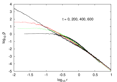
Figure 1: Spherically averaged density profile of a $N=1000$ star cluster (the average of 5 clusters) evolved starting from a Plummer sphere with core radius $r=3\pi/16$. (The total mass and energy of the cluster are 1 and $-1/4$, respectively; the crossing time is $t_{\rm cr}=2\sqrt{2}$ and the relaxation time is $t_{\rm rel}=0.1Nt_{\rm cr}/\ln N=41$.) Two-body scattering transfers heat out from the core of the cluster causing it to shrink and become increasingly dense until hard binaries form.

Modern computing power makes it almost possible (with approximate treatments of stellar evolution and tidal interactions) to study globular cluster dynamics directly using full numerical simulation HeggieHut . A more modest example illustrating the gravothermal instability is shown in Figure 1 using exact pairwise forces and a fourth-order symplectic integrator farrbert .

5 Dark Matter and Brownian Motion in the Early Universe

Most of the mass in the universe is in some form other than atomic (“baryonic”) matter. This matter is invisible — it neither scatters nor absorbs detectable amounts of electromagnetic radiation — and has been dubbed “dark matter.” Dark matter has been detected only through its gravitational effect on atomic matter and light. Its existence has been suspected for 70 years and known with confidence for about 25 years. However, the exact nature of dark matter is still unknown.

The most natural hypothesis is that dark matter consists of particles or fields not yet detected in the laboratory. Astrophysics and cosmology provide strong constraints on the nature of this substance. The particles (or field excitations) must have sufficiently small thermal speed to provide the seeds for galaxy formation. This rules out standard model neutrinos. It cannot be atomic matter in any form without having overproduced helium during big bang nucleosynthesis. While proposals have been made that dark matter is an illusion arising from modified gravity MOND , the only known theoretically and experimentally consistent implementation of modified gravity without dark matter Bekenstein is far less economical and less well tested than the dark matter hypothesis.

Dark matter is natural in extensions of the standard model particleDM , with two leading candidates: axions and WIMPs (weakly interacting massive particles). Axions are hypothetical ultra-low energy excitations of the $\theta$-vacuum of QCD that arise naturally as a solution of the strong CP problem (i.e., why the strong interactions conserve CP, or why the neutron has a tiny electric dipole moment). They are spin-0 particles of mass $10^{-6}$ to $10^{-2}$ eV and despite their light mass have negligible thermal speeds because they form a Bose-Einstein condensate.

WIMPs are popular dark matter candidates because supersymmetry and other extensions of the standard model of particle physics call for particles with approximately the correct mass and cross section to produce the observed abundance of dark matter LeeWeinberg . The favored dark matter candidate is the lightest neutralino $\chi^{0}$, the supersymmetric partner of a linear combination of the photon, $Z^{0}$, and Higgs bosons. The neutralino is spin-$\frac{1}{2}$, has mass $m_{\chi}$ in the range 20 to 500 GeV, and is its own antiparticle.

At present, these dark matter models are speculative. Proof will come only from direct detection of dark matter particles in the laboratory. Nonetheless, the models are sufficiently compelling to merit detailed examination of their astrophysical consequences. The remainder of this section focuses on WIMPS as they are better studied than axions.

WIMP dark matter may be effectively collisionless today, but in the early universe WIMPs scattered rapidly with fermions in the relativistic plasma. Inelastic processes such as $\chi^{0}\chi^{0}\leftrightarrow L\bar{L}$, where $L$ is a lepton, maintained the abundance of WIMPs in chemical equilibrium until the reaction rates fell below the Hubble expansion rate (chemical decoupling or freezeout). This happened after the WIMPs became nonrelativistic and their abundance decreased exponentially through annihilation. At a temperature $\sim m_{\chi}/25$, annihilation ceased to be effective and the abundance of WIMPs froze out to $n(\chi^{0})/n(L)\sim 10^{-10}$.

After annihilation ceased, WIMPS continued to undergo elastic scattering $\chi^{0}L\leftrightarrow\chi^{0}L$ with abundant leptons until the temperature had fallen to a few MeV (not coincidentally, slightly before neutrino decoupling at 2 MeV). During this period the WIMPs underwent Brownian motion as they were bombarded by the light relativistic leptons, with two important consequences. First, the WIMPs were maintained in kinetic (thermal) equilibrium with the relativistic plasma until the elastic scattering rate fell below the Hubble expansion rate (kinetic decoupling). Second, friction between the WIMPs and leptons damped density perturbations generated in the early universe. WIMP dark matter should therefore have a thermal cutoff in its perturbation spectrum at length scales corresponding roughly to the Hubble distance at kinetic decoupling.

The Brownian motion of WIMPs can be studied starting from the relativistic Boltzmann equation. Expanding the Boltzmann collision integral in powers of the momentum transfer divided by the WIMP mass, for nonrelativistic WIMPs one obtains the relativistic Fokker-Planck equation

$$\frac{Df}{d\tau} \equiv g^{\mu\nu}\left(p_{\mu}\frac{\partial f}{\partial x^{\nu}}+\Gamma^{\lambda}_{\ \,i\mu}p_{\lambda}p_{\nu}\frac{\partial f}{\partial p_{i}}\right)$$

$$=\left(\frac{df}{d\tau}\right)_{c} = \gamma\frac{\partial}{\partial{\bf p}}\cdot\left[({\bf p}-m_{\chi}{\bf v}_{L})f+m_{\chi}kT_{L}\frac{\partial f}{\partial{\bf p}}\right]\ ,$$ (18)

where $f({\bf x},{\bf p},t)$ is the distribution function in a local Lorentz frame, ${\bf v}_{L}$ and $T_{L}$ are the mean fluid velocity and temperature of the lepton fluid, and $\gamma$ is the collision rate coefficient determined from particle physics.

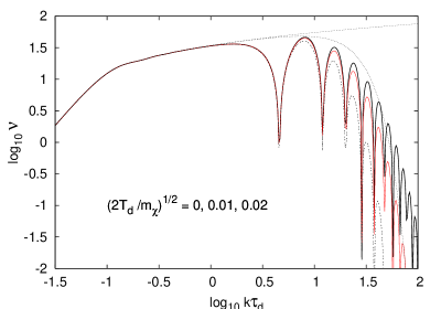
Figure 2: Cold dark matter density transfer function versus wavenumber (in units of the inverse decoupling time) after kinetic decoupling in the early universe; $\nu$ is the factor by which primordial fluctuations grow due to gravitational instability. Here $T_{d}$ is the temperature at which kinetic decoupling takes place; realistic models have $0.01<(2T_{d}/m_{\chi})^{1/2}<0.02$ (larger values of this parameter give more damping). The upper, monotonic curve assumes, unrealistically, that the dark matter is always collisionless and was never coupled to the radiation. The other non-oscillating curve shows a crude model of kinetic decoupling described by a Gaussian cutoff.

Equation (5) and the Einstein and fluid equations for the photon-lepton plasma have been solved numerically including the acoustic oscillations of the plasma before and during kinetic decoupling, the frictional damping occurring during kinetic decoupling, and the free-streaming damping occurring afterwards and throughout the radiation-dominated era b06 . For a $m_{\chi}=100$ GeV WIMP with bino-type interactions, kinetic decoupling occurs at a temperature $T_{d}=16$ MeV. Figure 2 shows the net effect of WIMP-lepton scattering on the linear transfer function of cold dark matter density perturbations. The damped oscillations are analogous to the acoustic peaks of the cosmic microwave background anisotropy and the baryon acoustic oscillations imprinted on the galaxy distribution. However, because WIMPs decouple at a redshift $z\sim 10^{10}$ instead of $z=1300$, the length scale of these fluctuations is about 1 pc instead of 100 Mpc. This length scale corresponds to a mass $10^{-4}\,(T_{d}/$10 MeV)^-3 M_⊙. It is possible, though at the moment controversial, that substructures as small as this might persist in our galaxy today and be detectable through the products of rare dark matter annihilations diemand .

6 Brownian Motion in Galaxy Formation

After kinetic decoupling in the early universe, dark matter dynamics is governed entirely by gravity. As shown above, stars undergo Brownian motion in a self-gravitating cluster. However, dark matter particles are much lighter than stars and their two-body interaction time is far longer than the age of the universe. Nonetheless, dark matter particles can scatter from quasiparticles or substructure in galaxy halos much as electrons scatter from substructure in the nucleon during deep inelastic scattering. In effect, galaxy halos are filled with gravitational partons.

The concept of dark matter substructure is based on the fact that nonlinear gravitational instability accumulates mass into dense clumps conventionally called dark matter halos (or minihalos or microhalos for the very small ones) ps74 . In the hierarchical clustering paradigm for structure formation, small-scale structures form first and then aggregate into larger objects where they persist for some time. Gravitational N-body simulations have shown that the spherically-averaged radial density profiles of the evolved halos take a nearly universal form nfw without providing an explanation for this result. One possibility is that scattering by substructure leads to relaxation.

The BBGKY hierarchy provides the exact statistical description for the evolution of a classical gas. The first BBGKY equation is similar to the Boltzmann equation except that it is exact, not phenomenological, and it is not closed:

$$\frac{\partial f}{\partial t}+{\bf v}\cdot\frac{\partial f}{\partial{\bf x}}+{\bf g}\cdot\frac{\partial f}{\partial{\bf v}}=-\frac{\partial}{\partial{\bf v}}\cdot{\bf F}_{v}\ ,\ \ \frac{\partial}{\partial{\bf x}}\cdot{\bf F}_{v}=4\pi G\rho_{2c}({\bf x},{\bf v},t)\ .$$ (19)

Here $\rho_{2c}$ is an integral over the phase-space two-point correlation function. The second BBGKY equation gives the evolution of the two-point correlation in terms of the three-point correlation, etc. For weakly correlated gases, these higher-order correlations may be neglected, and the two-point correlation term may be approximated by a Boltzmann collision integral. A different approach is needed for a gravitational plasma, where Boltzmann’s Stosszahlansatz does not apply.

In the early stages of gravitational clustering, $\rho_{2c}$ can be evaluated using second-order cosmological perturbation theory and the first BBGKY equation reduces to a Fokker-Planck equation mabert04 , with surprising results. First, the diffusivity eigenvalues can be negative, which appears to be a consequence of gravitational instability. Second, in the quasilinear regime there is no drag — $\gamma=0$ in equation (15) — but there is a nonzero radial drift ${\bf A}=A(r)\vec{e}_{r}$. Dynamical friction arises only in higher orders of perturbation theory (or in the fully nonlinear regime). The radial drift is induced by substructure. Finally, the timescale for relaxation obtained from the drift and diffusivity is the Hubble time, i.e. the collapse time of the initial perturbation. This initial relaxation is surprisingly fast.

The only approximation made in deriving this Fokker-Planck equation for dark matter evolution was second-order perturbation theory. The starting point was the exact BBGKY equation, not the phenomenological master equation, and there was no assumption of Markov dynamics. Indeed, the time evolution of a given realization of the random process is completely smooth. Why, then, is the system described by a Fokker-Planck equation? The answer is that the equation of motion for dark matter particles is a modified Langevin equation:

$$\frac{d{\bf v}}{dt}=-2H(t){\bf v}+b(t){\bf g}\ ,$$ (20)

where $H(t)$ is the Hubble expansion rate, $b(t)$ is proportional to the growth factor of density perturbations, and ${\bf g}({\bf x})$ is a Gaussian random field. For one realization of this process (i.e., one universe) this field is definite and the acceleration of every particle is smooth. The kinetic equation governs the evolution of the average dark matter halo, hence involves averaging over an ensemble of Gaussian random fields. This averaging leads to a Fokker-Planck equation.

The derivation suggests that spatial fluctuations of the density field can cause relaxation, but is not conclusive because the most important dynamical effects occur only in the fully nonlinear regime. Dynamical friction of substructure (both as “field” and “test” particles) and tidal stripping of substructure must be incorporated into the description. A major stumbling block is the statistical characterization of the substructure and its effects. Most investigations of substructure neglect velocity information, giving an inadequate description of phase space correlations. It remains to be seen whether a satisfactory kinetic theory can be devised for the fully nonlinear regime of dark matter gravitational clustering.

7 Conclusions

Brownian motion continues to serve as a paradigm for stochastic processes in physics and other disciplines. Einstein’s great insight was that the dynamics of Brownian motion can be understood by applying thermodynamic equilibrium to the interaction between a fluid of Brownian particles and the fluid in which those particles are suspended.

The universality of thermodynamics arises because most statistical systems near equilibrium relax at rates calculable from thermal equilibrium. Self-gravitating systems like globular star clusters and galaxies, with their negative specific heats and lack of thermodynamic equilibrium, are an important exception. While N-body simulations are the main tool for studying the evolution of self-gravitating systems, analytical insight can be obtained from kinetic theory, especially from the diffusive evolution driven by fluctuations.

A century after Einstein’s analysis of Brownian motion, the kinetic theory of self-gravitating systems remains a largely unsolved problem, presenting a great opportunity for a future Einstein — or a Fokker, Kramers, or Dupree.

References

- (1) A. Einstein, “ ber die von der molekularkinetischen Theorie der W rme geforderte Bewegung von in ruhenden Fl ssigkeiten Suspendierten Teilchen,” Ann. der Physik 17, 549–560 (1905).
- (2) A. Einstein, “Eine neue Bestimmung der Molek ldimensionen,” Ann. der Physik 19, 269–306 (1906); Erratum ibid., 34, 591–592 (1911).
- (3) A. Einstein, “Eine neue Bestimmung der Molek ldimensionen,” Ph.D. thesis, University of Z rich (July, 1905).
- (4) A. Einstein, Investigations on the Theory of Brownian Movement, edited by R. F rth and translated by A. D. Cowper, Dover, New York, 1956.
- (5) J. B. Perrin, “Mouvement brownien et réalité moléculaire,” Ann. de Chimie et Physique (VIII) 18, 5–114 (1909).
- (6) R. Brown, “A brief account of microscopical observations made in the months of June, July, and August, 1827, on the particles contained in the pollen of plants; and on the general existence of active molecules in organic and inorganic bodies,” Philos. Mag. (N. S.) 6, 161–173 (1828).
- (7) L. G. Gouy, “Note sur le Mouvement Brownien,” J. de Physique 7 [2], 561–564 (1888).
- (8) W. A. Sutherland, “A dynamical theory of diffusion for non-electrolytes and the molecular mass of albumin,” Philos. Mag. 9, 781–785 (1905).
- (9) M. von Smoluchowski,“Zur kinetischen Theorie der Brownschen Molekularbewegung und der Suspensionen,” Ann. der Physik 21, 756–780 (1906).
- (10) P. Hänggi and F. Marchesoni, “100 Years of Brownian Motion,” Chaos 15, 026101 (2005).
- (11) A. Pais, Subtle is the Lord, Oxford University Press, New York, 1982.
- (12) R. Newburgh, J. Peidle, and W. Rueckner, “Einstein, Perrin, and the reality of atoms: 1905 revisited,” Am. J. Phys. 74, 478–481 (2006).
- (13) P. Langevin, “Sur le théorie de mouvement brownien,” C.R. Acad. Sci. (Paris) 146, 530–533 (1908); see also D. S. Lemons and A. Gythiel, “Paul Langevin’s 1908 paper ‘On the theory of Brownian motion,’” Am. J. Phys. 65, 1079–1081 (1997).
- (14) Yu. L. Klimontovich, The Statistical Theory of Non-Equilibrium Processes in a Plasma, MIT Press, Cambridge, 1967.
- (15) T. H. Dupree, “Nonlinear Theory of Drift-Wave Turbulence and Enhanced Diffusion,” Phys. Fluids 10, 1049–1055 (1967).
- (16) A. D. Fokker, “Die mittlere Energie rotierender elektrischer Dipole im Strahlungsfeld,” Ann. der Physik, 43, 810–820 (1914); M. Planck, “ ber einen Satz der statistischen Dynamik and seine Erweiterung in der Quantentheorie,” Sitzungsber. Preuss. Akad. Wiss., 324–341 (1917).
- (17) H. A. Kramers, “Brownian motion in a field of force and the diffusion model of chemical reactions,” Physica 7, 284–304 (1940).
- (18) C. W. Gardiner, Handbook of Stochastic Methods, Springer, Berlin, 2004.
- (19) H. Risken, The Fokker-Planck Equation, Springer-Verlag, New York, 1996.
- (20) D. Pooley et al., “Dynamical Formation of Close Binary Systems in Globular Clusters,” Astrophys. J. 591, L131–L134 (2003); D. Pooley and P. Hut, “Dynamical Formation of Close Binaries in Globular Clusters: Cataclysmic Variables,” Astrophys. J. 646, L143–L146 (2006).
- (21) A. C. Fabian, J. E. Pringle, and M. J. Rees, “Tidal capture formation of binary systems and X-ray sources in globular clusters,” Mon. Not. R. Astron. Soc. 172, 15p–18p (1975); D. C. Heggie, “Binary evolution in stellar dynamics,” Mon. Not. R. Astron. Soc. 173, 729–787 (1975).
- (22) D. Lyden-Bell and R. Wood, “The gravo-thermal catastrophe in isothermal spheres and the onset of red-giant structure for stellar systems,” Mon. Not. R. Astron. Soc. 138, 495–525 (1968).
- (23) S. Chandrasekhar, “Stochastic Problems in Physics and Astronomy,” Rev. Mod. Phys. 15, 1–89 (1943); “Dynamical Friction. I. General Considerations: the Coefficient of Dynamical Friction,” Astrophys. J. 97, 255–262 (1943); M. N. Rosenbluth, W. M. MacDonald, and D. L. Judd, “Fokker-Planck Equation for an Inverse-Square Force,” Phys. Rev. 107, 1–6 (1957).
- (24) D. Heggie and P. Hut, The Gravitational Million-Body Problem, Cambridge University Press, Cambridge, 2003.
- (25) W. Farr and E. Bertschinger, in preparation (2006).
- (26) M. Milgrom, “A modification of the Newtonian dynamics as a possible alternative to the hidden mass hypothesis,” Astrophys. J. 270, 365–370 (1983); R. H. Sanders and S. S. McGaugh, “Modified Newtonian Dynamics as an Alternative to Dark Matter,” Ann. Rev. Astron. Astrophys. 40, 263–317 (2002).
- (27) J. D. Bekenstein, “Relativistic gravitation theory for the modified Newtonian dynamics paradigm,” Phys. Rev. D70, 083509 (2004); Erratum ibid., 71, 069901 (2004).
- (28) L. Bergstrom, “Non-Baryonic Dark Matter - Observational Evidence and Detection Methods,” Rep. Prog. Phys. 63, 793–841 (2000); G. Bertone, D. Hooper, and J. Silk, “Particle Dark Matter: Evidence, Candidates and Constraints,” Phys. Rep. 405, 279–390 (2005).
- (29) B. W. Lee and S. Weinberg, “Cosmological Lower Bound on Heavy-Neutrino Masses,” Phys. Rev. Lett. 39, 165–168 (1977); G. Jungman, M. Kamionkowski, and K. Griest, “Supersymmetric Dark Matter,” Phys. Rep. 267, 195–373 (1996).
- (30) E. Bertschinger, “The Effects of Cold Dark Matter Decoupling and Pair Annihilation on Cosmological Perturbations,” Phys. Rev. D, 74, in press (astro-ph/0607391).
- (31) J. Diemand, B. Moore, and J. Stadel, “Earth-mass dark-matter haloes as the first structures in the early Universe,” Nature 433, 389–391 (2005).
- (32) P. Schechter and W. H. Press, “Formation of Galaxies and Clusters of Galaxies by Self-Similar Gravitational Condensation,” Astrophys. J. 187, 425–438 (1974).
- (33) J. F. Navarro, C. S. Frenk, and S. D. M. White, “The Structure of Cold Dark Matter Halos,” Astrophys. J. 462, 563–575 (1996); “A Universal Density Profile from Hierarchical Clustering,” Astrophys. J. 490, 493–508 (1997).
- (34) C.-P. Ma and E. Bertschinger, “A Cosmological Kinetic Theory for the Evolution of Cold Dark Matter Halos with Substructure: Quasi-Linear Theory,” Astrophys. J. 612, 28–49 (2004).