Hardness Ratio Estimation in Low Counting X-ray Photometry

Abstract

Hardness ratios are commonly used in X-ray photometry to indicate spectral properties roughly. It is usually defined as the ratio of counts in two different wavebands. This definition, however, is problematic when the counts are very limited. Here we instead define hardness ratio using the $\lambda$ parameter of Poisson processes, and develop an estimation method via Bayesian statistics. Our Monte Carlo simulations show the validity of our method. Based on this new definition, we can estimate the hydrogen column density for the photoelectric absorption of X-ray spectra in the case of low counting statistics.

1 Introduction

In recent years, high angular resolution X-ray telescopes make it possible to detect X-ray sources with only a few counts. This is very different from the optical photometry. Because of these low counts, the Poisson processes in corresponding wavebands cannot be approximated to Gaussian distribution. Therefore the statistics will be very different in some estimations and calculations than used before. In recent years Bayesian method has gained many applications (e.g. van Dyk et al. 2001 and references therein) since it has more advantages in low count cases than traditional statistics.

Hardness ratios are widely used in high energy astrophysics since faint sources with only limited counts cannot give any satisfying spectral modeling. In X-ray detection, hardness ratios are normally used to show spectral properties roughly (e.g. Tennant et al., 2001; Sivakoff, Sarazin & Carlin 2004). Hardness ratios are usually defined as the ratio of counts in different wavebands ($HR=b/a$) or the ratio of the difference and sum of counts in two wavebands ($HR=(b-a)/(b+a)$), $a$ and $b$ are counts in two wavebands $A$ and $B$. On the other hand, for the spectra of X-ray sources, the photoelectric absorption, quantified with the hydrogen column density $N_{H}$, cannot be neglected. Hydrogen column density contains many kinds of important information, such as the radial distance and the interstellar circumstance of the sources. For low count sources, hydrogen column density is hard to know since no reliable spectral fitting can be made. However interstellar absorption is energy dependent. Consequently the information of hydrogen column density can be drawn from the hardness ratios. In this paper, we first give a new definition of hardness ratio and its estimation method, and then we discuss the procedure to estimate the hydrogen column density accordingly.

2 The distribution of $\lambda$ parameter under certain counts

We begin our discussion with the following problem: Suppose that one experiment obtained two counts from two different Poisson distributions, we need to: (1) Estimate the ratio of the expectation values of the two Poisson distributions, and (2) Construct the confidence interval of the ratio.

The expectation values of the Poisson processes are just the $\lambda$ parameters of the Poisson distribution $P(n|\lambda)=\frac{\lambda^{n}}{n!}e^{-\lambda}$. Therefore the above problem may be formulated as follows: Suppose $a$ and $b$ are two counts corresponding to two different Poisson processes $A$ and $B$ with their parameters as $\lambda_{A}$ and $\lambda_{B}$ respectively, $\lambda_{A}/\lambda_{B}$ and its confidence interval needs to be estimated. To solve this problem we first need to derive the distribution of $\lambda$ parameter under certain counts, i.e., the conditional distribution of $\lambda_{A}$ and $\lambda_{B}$, as follows.

$$p(\lambda_{A}=x|n_{A}=a) = \frac{P(n_{A}=a|\lambda_{A}=x)p(\lambda_{A}=x)}{\int_{0}^{\infty}P(n_{A}=a|\lambda_{A}=t)p(\lambda_{A}=t){\rm d}t}.$$ (1)

First we assume, as a pragmatic convention, a uniform prior for the $\lambda$ parameter.

$$p_{u}(\lambda_{A}=x|n_{A}=a) = \frac{P(n_{A}=a|\lambda_{A}=x)}{\int_{0}^{\infty}P(n_{A}=a|\lambda_{A}=t){\rm d}t}$$ (2)

$$= \frac{x^{a}e^{-x}}{a!}.$$

Similarly,

$$p_{u}(\lambda_{B}=y|n_{B}=b) = \frac{y^{b}e^{-y}}{b!}.$$ (3)

This continuous distribution is Gamma distribution, as shown in Fig. 1.

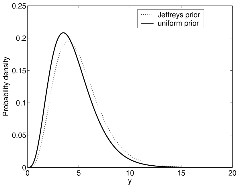
Figure 1: The probability density function of $\lambda_{B}$ when $b=4$ under the two different prior assumption.

In addition, we use Jeffreys prior ($p(\lambda)=1/\sqrt{\lambda}$), which may be more advantageous over the uniform prior commonly used, because the inferences derived from Jeffreys prior are parameterization-invariant (See Kass & Wasserman 1996 for detail of this prior). Under this prior, the conditional distribution of $\lambda$ is

$$p_{J}(\lambda_{A}=x|n_{A}=a) = \frac{P(n_{A}=a|\lambda_{A}=x)(1/\sqrt{x})}{\int_{0}^{\infty}P(n_{A}=a|\lambda_{A}=t)(1/\sqrt{t}){\rm d}t}$$ (4)

$$= \frac{2^{a}x^{a-1/2}e^{-x}}{(2a-1)!!\sqrt{\pi}},$$

and

$$p_{J}(\lambda_{B}=x|n_{B}=b) = \frac{2^{b}x^{b-1/2}e^{-x}}{(2b-1)!!\sqrt{\pi}}.$$ (5)

To account for the background contamination, suppose that $a$ is the count corresponding to a Poisson process $A$ with the addition of a Poisson background process $A_{bkg}$, the expectation value of the process $A_{bkg}$ is assumed to be known as $\lambda_{Ab}$. According to the properties of Poisson processes, the sum of two Poisson processes is also a Poisson process with the parameter $\lambda_{A}+\lambda_{Ab}$. So the probability of the total count $n$ is $P(n=a|\lambda_{A}=x,\lambda_{Ab})=\frac{(x+\lambda_{Ab})^{a}}{a!}e^{-(x+\lambda_{Ab})}$. Apply the Bayesian assumption and the uniform prior distribution assumption, we obtain the conditional distribution of $\lambda_{A}$, as follows.

$$p_{u}(\lambda_{A}=x|n_{A}=a,\lambda_{Ab}) = \frac{P(n_{A}=a|\lambda_{A}=x,\lambda_{Ab})p_{u}(\lambda_{A}=x)}{\int_{0}^{\infty}P(n_{A}=a|\lambda_{A}=t,\lambda_{Ab})p_{u}(\lambda_{A}=t){\rm d}t}$$ (6)

$$= \frac{P(n_{A}=a|\lambda_{A}=x,\lambda_{Ab})}{\int_{0}^{\infty}P(n_{A}=a|\lambda_{A}=t,\lambda_{Ab}){\rm d}t}$$

$$= \frac{(x+\lambda_{Ab})^{a}e^{-x}}{a!\sum\limits_{k=0}^{a}(\frac{\lambda_{Ab}^{k}}{k!})}.$$

When $\lambda_{Ab}$ is much smaller than $a$, this result is same as equation(2). Also we can obtain the conditional distribution under the Jeffreys prior distribution assumption,

$$p_{J}(\lambda_{A}=x|n_{A}=a,\lambda_{Ab}) = \frac{(x+\lambda_{Ab})^{a}e^{-x}(1/\sqrt{x})}{\int_{0}^{\infty}(t+\lambda_{Ab})^{a}e^{-t}(1/\sqrt{t})dt},$$ (7)

and it is same as equation(4) when $\lambda_{Ab}$ is much smaller than $a$.

3 Estimate the Hardness Ratio

There are two different definitions of hardness ratio, $R=\lambda_{A}/\lambda_{B}$ and $HR=(\lambda_{B}-\lambda_{A}/)/(\lambda_{B}+\lambda_{A})$. In traditional method, the estimate of $R$ and $HR$ are $a/b$ and $(b-a)/(b+a)$ respectively, and the errors are propagated under the Gaussian distribution, i.e.,

$$\sigma_{R} = \frac{a}{b}\sqrt{\frac{\sigma_{a}^{2}}{a^{2}}+\frac{\sigma_{b}^{2}}{b^{2}}},$$

$$\sigma_{HR} = \frac{2\sqrt{b^{2}\sigma_{a}^{2}+a^{2}\sigma_{b}^{2}}}{(b+a)^{2}}.$$ (8)

Here we propose a method to estimate the hardness ratio based on the Bayesian method. Both the uniform prior and the Jeffreys prior will be used. When $\lambda_{Ab}$ is much smaller than $a$, we use equation(2) (under the uniform prior) or equation(4) (under the Jeffreys prior) to estimate $R=\lambda_{A}/\lambda_{B}$ and $HR=(\lambda_{B}-\lambda_{A})/(\lambda_{B}+\lambda_{A})$.

First we assume the uniform prior of $\lambda$. For the conditional distribution function of $\lambda_{A}/\lambda_{B}$,

$$P_{u}(\frac{\lambda_{A}}{\lambda_{B}}\leq z) = \int_{0}^{\infty}P(\frac{\lambda_{A}}{\lambda_{B}}\leq z|\lambda_{B}=y)p_{u}(\lambda_{B}=y){\rm d}y$$ (9)

$$= \int_{0}^{\infty}(\int_{0}^{zy}\frac{x^{a}e^{-x}}{a!}{\rm d}x)\frac{y^{b}e^{-y}}{b!}{\rm d}y.$$

For the conditional probability density function of $\lambda_{A}/\lambda_{B}$,

$$p_{u}(\frac{\lambda_{A}}{\lambda_{B}}=z) = \frac{\rm d}{{\rm d}z}P_{u}(\frac{\lambda_{A}}{\lambda_{B}}\leq z)$$ (10)

$$= \frac{\rm d}{{\rm d}z}\int_{0}^{\infty}(\int_{0}^{zy}\frac{x^{a}e^{-x}}{a!}{\rm d}x)\frac{y^{b}e^{-y}}{b!}{\rm d}y$$

$$= \int_{0}^{\infty}(\frac{\partial}{\partial z}\int_{0}^{zy}\frac{x^{a}e^{-x}}{a!}{\rm d}x)\frac{y^{b}e^{-y}}{b!}{\rm d}y$$

$$= \int_{0}^{\infty}\frac{{(zy)}^{a}e^{-zy}}{a!}y\frac{y^{b}e^{-y}}{b!}{\rm d}y$$

$$= \frac{z^{a}(a+b+1)!}{(z+1)^{a+b+2}a!b!}.$$

This distribution is shown in Fig. 2 when $a=4$, $b=3$. It is easy to verify that the distribution is normalized,

$$\int_{0}^{\infty}\frac{z^{a}(a+b+1)!}{(z+1)^{a+b+2}a!b!}{\rm d}z=1.$$ (11)

For the hardness ratio $HR$, the probability distribution of this hardness ratio is given by,

$$P_{u}(\frac{\lambda_{B}-\lambda_{A}}{\lambda_{B}+\lambda_{A}}\leq z) = \int_{0}^{\infty}P(\frac{\lambda_{B}-\lambda_{A}}{\lambda_{B}+\lambda_{A}}\leq z|\lambda_{A}=x)p_{u}(\lambda_{A}=x){\rm d}x$$ (12)

$$= \int_{0}^{\infty}P(\lambda_{B}\leq\frac{1+z}{1-z}\lambda_{A}|\lambda_{A}=x)p_{u}(\lambda_{A}=x){\rm d}x$$

$$= \int_{0}^{\infty}(\int_{0}^{\frac{1+z}{1-z}x}\frac{y^{b}e^{-y}}{b!}{\rm d}y)\frac{x^{a}e^{-x}}{a!}{\rm d}x.$$

The conditional probability density function is given by,

$$p_{u}(\frac{\lambda_{B}-\lambda_{A}}{\lambda_{B}+\lambda_{A}}=z) = \frac{\rm d}{{\rm d}z}P_{u}(\frac{\lambda_{B}-\lambda_{A}}{\lambda_{B}+\lambda_{A}}\leq z)$$ (13)

$$= \frac{\rm d}{{\rm d}z}\int_{0}^{\infty}(\int_{0}^{\frac{1+z}{1-z}x}\frac{y^{b}e^{-y}}{b!}{\rm d}y)\frac{x^{a}e^{-x}}{a!}{\rm d}x$$

$$= \int_{0}^{\infty}(\frac{\partial}{\partial z}\int_{0}^{\frac{1+z}{1-z}x}\frac{y^{b}e^{-y}}{b!}{\rm d}y)\frac{x^{a}e^{-x}}{a!}{\rm d}x$$

$$= \int_{0}^{\infty}\frac{{(\frac{1+z}{1-z}x)}^{b}e^{-\frac{1+z}{1-z}x}}{b!}\frac{2x}{(1-z)^{2}}\frac{x^{a}e^{-x}}{a!}{\rm d}x$$

$$= \frac{(1-z)^{a}(1+z)^{b}(a+b+1)!}{2^{(a+b+1)}a!b!}.$$

This distribution is shown in Fig. 3 when $a=4$, $b=3$. It is easy to verify that the distribution is normalized,

$$\int_{0}^{\infty}\frac{(1-z)^{a}(1+z)^{b}(a+b+1)!}{2^{(a+b+1)}a!b!}{\rm d}z=1.$$ (14)

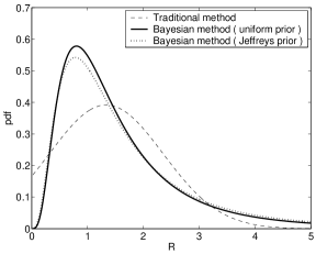
Figure 2: The probability density function of $\lambda_{A}/\lambda_{B}$ when $a=4$, $b=3$. The solid line represents the distribution derived by our proposed method under the uniform prior, the doted line represents the distribution derived by our proposed method under the Jeffreys prior, the dashed line represents the Gaussian distribution derived by the traditional method.

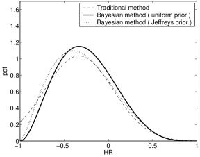
Figure 3: The probability density function of $(\lambda_{B}-\lambda_{A})/(\lambda_{B}+\lambda_{A})$ when $a=4$, $b=3$.The solid line represents the distribution derived by our proposed method under the uniform prior, the doted line represents the distribution derived by our proposed method under the Jeffreys prior, the dashed line represents the Gaussian distribution derived by the traditional method.

Similarly, we obtain the conditional probability density function of $R$ and $HR$ under the Jeffreys prior assumption as follows,

$$p_{J}(R=z) = \frac{z^{a-1/2}2^{a+b}(a+b)!}{(z+1)^{a+b+1}(2a-1)!!(2b-1)!!\pi},$$ (15)

and

$$p_{J}(HR=z) = \frac{(1-z)^{a-1/2}(1+z)^{b-1/2}(a+b)!}{(2a-1)!!(2b-1)!!\pi}.$$ (16)

Using the result of $p(R=z)$ and $p(HR=z)$, we can estimate $R$ and $HR$.

Under the uniform prior assumption, since we have only one observation, we take the most probable value as the estimate of $R=\lambda_{A}/\lambda_{B}$, denoted as $(z_{R})_{u}$. Let

$$\frac{\partial}{\partial z}p_{u}(\frac{\lambda_{A}}{\lambda_{B}}=z|n_{A}=a,n_{B}=b) = 0,$$ (17)

we obtain,

$${(z_{R})_{u}} = \frac{a}{b+2}.$$ (18)

Similarly, we obtain the most probable value as the estimate of HR:

$${(z_{HR})_{u}} = \frac{b-a}{b+a}.$$ (19)

Similarly, we get the most probable value of $R$ and $HR$ under the Jeffreys prior assumption,

$${(z_{R})_{J}} = \frac{a-1/2}{b+3/2},$$ (20)

and

$${(z_{HR})_{J}} = \frac{b-a}{b+a-1}.$$ (21)

The highest posterior density (HPD) interval is used to give the error bars. The HPD interval under the confidence level $\alpha$ is the range of values which contain a fraction $\alpha$ of the probability, and the probability density within this interval is always higher than that outside the interval.

There are other point estimates and error estimates. For example, the mean value and the equal tailed interval. Since the distributions of $R$ and $HR$ are obtained, these alternative estimates can be easily derived.

When $\lambda_{Ab}$ cannot be ignored, equation (6) or equation (7) can be used to estimate $R$ and $HR$. In this situation, it is difficult to give a simple analytic distribution function like equation (10) or equation (13); in this case, one can only use numerical integration to obtain the distribution of $R$ and $HR$, and then do the estimate.

4 Frequency Properties of Intervals

We use the Monte Carlo simulations to investigate the statistical properties of our result, and compare them with the traditional methods.

First we set $\lambda_{A}$ and $\lambda_{B}$. Do Poisson sampling for $N$ times and each time we get $a$ and $b$ respectively. Each time we estimate $R$ and $HR$ using two kinds of methods. Finally we obtain that, for two methods, the mean square error of the point estimate, the coverage rate (the percentage of times during which the confidence interval contains the real value), and the mean confidence interval.

The simulations contain two cases: low counts and high counts. In case 1, we first set $\lambda_{A}=3$ and $\lambda_{B}=3$, then set $\lambda_{A}=4$ and $\lambda_{B}=3$. In case 2, we first set $\lambda_{A}=20$ and $\lambda_{B}=20$, then set $\lambda_{A}=20$ and $\lambda_{B}=15$. The confidence level in the simulations is 90%. The results of the simulations are shown in table 1.

Table 1: Statistical Properties of Our Method and Traditional Method.

			Low counts		High counts
			1:1	4:3	1:1	4:3
	our method	R	0.5291	0.6872	0.3066	0.4397
mean square error	traditional method	R	1.2399	1.5308	0.3628	0.5767
	our method	R	94.62%	89.13%	93.00%	90.00%
	(uniform prior)	HR	94.38%	91.49%	85.90%	85.00%
	our method	R	92.27%	92.35%	91.30%	87.87%
	(Jeffreys prior)	HR	82.82%	87.52%	87.50%	84.62%
coverage rate	traditional	R	84.70%	84.82%	90.29%	89.46%
	method	HR	88.22%	85.34%	89.10%	88.26%
	our method	R	3.40	4.67	1.20	1.60
	(uniform prior)	HR	1.06	1.00	0.50	0.53
	our method	R	4.05	5.56	1.17	1.80
mean	(Jeffreys prior)	HR	1.13	1.05	0.50	0.56
confidence interval	traditional	R	4.91	5.90	1.17	1.78
	method	HR	1.43	1.23	0.52	0.55

From the simulation results, we notice that our proposed method is more reliable than the traditional method when the counts are low. The reason is that the traditional method is based on using the Gaussian distribution to approach the Poisson distribution, which is not reliable when the counts are low.

5 Application to $N_{H}$ Estimation

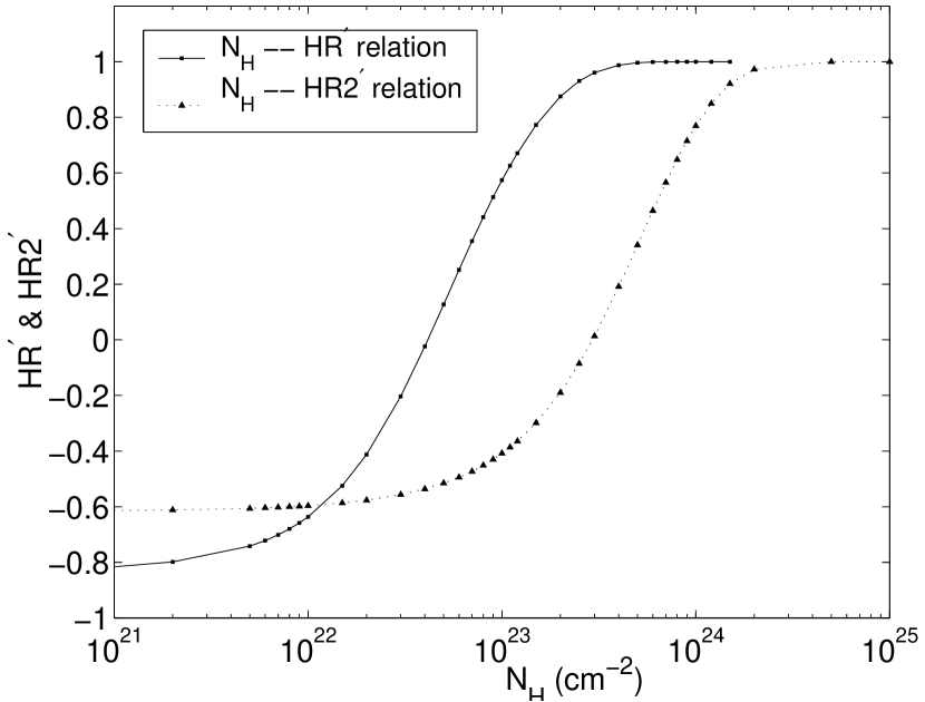
Figure 4: Relation between $N_{H}$ and $HR^{\prime}$ & $HR2^{\prime}$. The solid line with squares is the relation of $N_{H}$ and $HR^{\prime}$, while the dotted line with triangles is the one of $N_{H}$ and $HR2^{\prime}$ (Wu et al. 2006)

Here we propose a method to estimate the hydrogen column density using data obtained with the Chandra X-ray observatory. Because of the high angular resolution of Chandra, a positive detection of a point source during a survey observation only requires several counts. Therefore our method will be more reliable when estimating the hardness ratio than the traditional method. The detail procedure of this application can be found in another paper (Wu et al. 2006). The basic idea is introduced as follows.

The basic procedure consists of the following three steps: (1) calculate the relationship between the hardness ratios and $N_{H}$ values under certain spectral model; (2) estimate hardness ratios according to observed counts in different wavebands; and (3) interpolate the $N_{H}$ values and error intervals from hardness ratios.

According to the most likely physical nature of the sources, we can assume a spectral model (e.g. power law with photon index $\Gamma=2$ for typical X-ray binaries). Then we can use PIMMS (http://cxc.harvard.edu/toolkit/pimms.jsp) tool to calculate the relationship between hydrogen column density and the hardness ratio. Using PIMMS, one can get the count rate in certain energy band under a given X-ray spectrum and hydrogen column density. The count rate in the given energy band is just the $\lambda$ parameter in this energy band; this was our original movivation of defining the hardness ratios in terms of the $\lambda$ parameter. The calculated $N_{H}$ (hydrogen column density) — $HR$ relationships are shown in Fig. 7 for three different energy bands of $A$ (1 - 3 keV), $B$ (3 - 5 keV) and $C$ (5 - 8 keV) for a Chandra ACIS-I observation (Wu et al. 2006) respectively: $HR^{\prime}=\frac{\lambda_{B}-\lambda_{A}}{\lambda_{B}+\lambda_{A}}$, $HR2^{\prime}=\frac{\lambda_{C}-\lambda_{B}}{\lambda_{C}+\lambda_{B}}$. From Fig. 7, we can see that $HR^{\prime}$ or $HR2^{\prime}$ is more appropriate for $N_{H}<2\times 10^{23}{\rm cm}^{-2}$ or $N_{H}>2\times 10^{23}{\rm cm}^{-2}$, respectively. Having the value and error interval of $HR$, we can finally do linear interpolation on curves in Fig. 7 to obtain the value and error interval of hydrogen column density.

6 Summary & Discussion

First we give the conditional probability distribution of $\lambda$ parameter under certain counts in a Poisson process using Bayesian statistics. According to this result we derive the probability density function of two kinds of hardness ratios. We take the most probable values as the estimate of hardness ratios and the HPD intervals as the error intervals. Then we use Monte Carlo simulations to investigate the statistical properties of our results, and find that our method is more reliable than the traditional method when the counts are low. Finally we show how to estimate the hydrogen column density using hardness ratios.

Our method developed in this paper provides a way to estimate the hydrogen column density of sources which are too faint to do spectral fitting. However the spectral shape for these sources must be assumed a prior. This method is especially convenient for a sample of faint sources with similar spectra.

After this paper has been submitted initially on 06-03-29, we noticed another submitted paper (Park et al. 2006) which discusses the same statistical problem as we have done in this paper. In that paper the authors also used the Bayesian method to estimate the hardness ratio, and showed some applications on quiescent Low-Mass X-ray Binaries, the evolution of a flare, etc, therefore justifying the wide range of applications of such a statistical problem. Since the strict analytic solution of the hardness ratio distribution does not exist for general situations, the authors suggested methods by Monte Carlo and numerical integration to obtain the distribution in that paper. In our paper we find simple analytic solutions of the probability density functions of hardness ratios for the situations in which the background can be ignored. This will be useful and convenient for some applications, such as Chandra data in which background can be ignored for hardness ratio estimation of point sources.

Finally, we note, under the advise of the referee, that in 1980s some studies have been done on the ratio of Poisson means both from a frequentist standpoint (James & Roos 1980) and from a Bayesian standpoint (Helene 1984 and Prosper 1985). In this paper we used the Bayesian method under the uniform prior and the Jeffreys prior, made extensive comparisons between this method and traditional method, aiming explicitly at applications in astrophysics.

References

- (1) Kass, R. E., & Wasserman, L., 1996, J. Amer. Statist. Ass. 91, 1343
- (2) James, F., & Roos, M., 1980, Nucl. Phys. B172, 475
- (3) Helene, O., 1984, Nucl. Instr. and Meth. A228, 120
- (4) Prosper, H. B., 1985, Nucl. Instr. and Meth. A241, 236
- (5) Park, T., Kashyap, V. L., Siemiginowska, A., Dyk, D. A. V., Zezas, A., Heinke, C., & Wargelin, B. J., 2006, submitted to ApJ (arXiv:astro-ph/0606247)
- (6) Sivakoff, G. R., Sarazin, C. L., & Carlin, J. L., 2004, ApJ, 617, 262
- (7) Tennant, A. F., Wu, K., Ghosh, K. K., Kolodziejcazk, J. J., & Swartz, D. A., 2001, ApJ, 549, L43
- (8) van Dyk, D. A., Connors, A., Kashyap, V. L., & Siemiginowska, A., 2001, ApJ, 548, 224
- (9) Wu, J. F., Zhang, S. N., Lu, F. J., & Y. K. Jin, 2006, accepted for publication in Chinese Journal of Astronomy and Astrophysics ( arXiv:astro-ph/0606478)