Coherent Synchrotron Radiation for Laminar Flows

Abstract

We investigate the effect of shear in the flow of charged particle equilibria that are unstable to the Coherent Synchrotron Radiation (CSR) instability. Shear may act to quench this instability because it acts to limit the size of the region with a fixed phase relation between emitters. The results are important for the understanding of astrophysical sources of coherent radiation where shear in the flow is likely.

I Introduction

When the wavelength of synchrotron radiation emitted by a bunch of relativistic particles is comparable to the size of the bunch the particles may radiate coherently. The coherent emission produces significantly greater power than the incoherent emission. Coherent synchrotron emission is seen from different astrophysical source but most notably from the rotationally powered radio pulsars (e.g., Manchester & Taylor (1977)). In particle accelerators the coherent synchrotron emission is usually undesirable because it causes very rapid energy loss. In this context we would also like to mention efforts to study coherent curvature radiation as a pulsar emission mechanism in the laboratory benford1981 .

Several effects may act to stabilize a system unstable to the CSR instability. In Schmekel:2004jb the authors analyzed the influence of a small energy spread in a beam of charged particles in approximately circular motion. A distribution function with a single value of the canonical angular momentum was considered. The radial width of the beam was given by the amplitude of the betatron oscillations which is non-zero for a non-zero energy spread. It was shown that the decoherence introduced by the betatron oscillations leads to a characteristic frequency spectrum, whereas the dependence on the Lorentz factor and the number density remains unaffected.

In this paper we relax the assumption of zero spread in the canonical angular momentum $P_{\phi}$ of the equilibrium distribution. In general this leads to shear in that the average angular velocity becomes dependent on the radius of the orbit. In practice the requirement of a small spread in the canonical angular momentum may be harder to satisfy than a small energy spread. Shear is expected in astrophysical sources of coherent emission arons1979 .

Shear itself can be the cause of instabilities, for example, the “diocotron instability” Davidson2001 , but this is not the focus of the present paper. In the case of CSR it is reasonable to expect that the shear acts to stabilize the CSR instability due to particles with different radii “slipping away”. Using a linear perturbation analysis of the fluid equations for a laminar Brillioun flow we show that even with a spread of the canonical angular momentum $\Delta P_{\phi}>0$, previous results for equilibria with constant $P_{\phi}$ can be recovered treating the plasma as a relativistic cold fluid. Computer simulations of CSR emission in Brillioun flows Schmekel:2004su are compatible with this picture. With the cold fluid approximation adopted here, the stability depends on the number density and the angular velocity which depends on the radius. The azimuthal velocity is approximately equal to the speed of light.

The problem of CSR emission has been investigated by several authors. Goldreich and Keeley GoldreichKeeley1971 considered the stability of a charge distribution whose motion is confined to a thin ring with the particle motion being one-dimensional. This calculation led to confusion as to how the proposed CSR mechanism works in detail (cf. buschauer1978 ).

As proposed in Schmekel:2004jb the CSR instability is related to the classical negative mass instability Nielson1959 ; Briggs1966 ; Entis1971 ; Kolomenskii1959 in the sense that an increase in particle energy leads to a decrease in its angular velocity. While the classical negative mass instability is caused by the Coulomb part of the electromagnetic potential, the CSR instability is caused by the radiation field. The negative mass effect is not immediately apparent in a one-dimensional treatment based on conservation of energy and charge. Heifets and Stupakov Heifets:2002un effectively built in the negative mass effect by hand having a constrained radius and particle energy.

The treatments GoldreichKeeley1971 ; Heifets:2002un ; Schmekel:2004jb give the growth rate in the absence of an energy spread. However, considering a non-zero energy spread requires a truly two-dimensional model. Larroche and Pellat investigated the effect of steep boundaries in the particle distribution function larroche1987 .

Section II describes the assumed models, and Section III approximate solutions of the equations. Section IV derives a dispersion relation for the considered perturbation. Section V discusses the results.

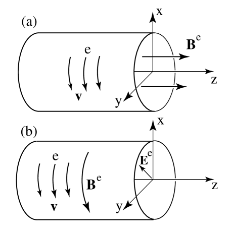
Figure 1: Panel (a) shows the geometry of a relativistic E-layer for the case of a uniform external axial magnetic field. Panel (b) shows the second case of a relativistic E-layer in an external toroidal magnetic field and an external radial electric field.

II Theory

We consider two cases illustrated in Figure 1. The first case (a) corresponds to a thin layer of relativistic electrons gyrating in a uniform external magnetic field, an “E-layer.” The second case (b) corresponds to the electrons moving almost parallel to a toroidal magnetic field.

II.1 Case a

We consider a laminar Brillioun type equilibrium of a long, non-neutral, cylindrical relativistic electron (or positron) layer in a uniform external magnetic field ${\bf B}_{e}=B_{e}\hat{\bf z}$, where we use a non-rotating cylindrical $(r,\phi,z)$ coordinate system. The electron velocity is ${\bf v}=v_{\phi}(r)\hat{{\hbox{\tenbg\char 30\relax}}~{}}=r\Omega(r)\hat{{\hbox{\tenbg\char 30\relax}}~{}}$ The self-magnetic field is in the $z-$direction while the self-electric field is in the $r-$direction. The radial force balance of the equilibrium is

$$-\gamma\Omega^{2}r={q\over m_{e}}(E+vB)~{},$$ (1)

where $\gamma=(1-v_{\phi}^{2})^{-1/2}$ is the Lorentz factor with velocities measured in units of the speed of light, $B=B_{e}+B_{s}$ is the total (self plus external) axial magnetic field, $E$ is the total ($=$ self) radial electric field, and $q$ and $m_{e}$ are the particle charge and rest mass. We have

$${1\over r}{d(rE)\over dr}=4\pi\rho_{e}~{},\quad{dB\over dr}=-4\pi\rho_{e}v~{},$$ (2)

where $\rho_{e}(r)$ is the charge density of the electron layer.

We consider weak layers in the sense that the ‘field reversal’ parameter

$$\zeta\equiv-~{}{4\pi\over B_{e}}\int_{r_{1}}^{r_{2}}dr\rho_{e}v$$ (3)

is small compared with unity, $\zeta^{2}\ll 1$. Under this condition equation 1 gives $\Omega=-qB_{e}/(m_{e}\gamma)$. Here, we have assumed that the layer exists between $r_{1}$ and $r_{2}$. We also consider that the Lorentz factor is appreciably larger than unity in the sense that $\gamma^{2}\gg 1$. Furthermore, we consider radially thin layers

$$\delta\equiv\frac{\Delta r}{r_{0}}\ll 1~{}.$$ (4)

We consider general electromagnetic perturbations of the electron layer with the perturbations proportional to

$$f_{\alpha}(r)\exp(im\phi-i\omega t)~{},$$ (5)

where $\alpha=1,2,..$ for the different scalar quantities, $m=$ integer, and $\omega$ the angular frequency of the perturbation. Thus the perturbations give rise to field components $\delta E_{r}$, $\delta E_{\phi}$, and $\delta B_{z}$. The perturbed equation of motion is

$$\left({\partial\over\partial t}+{\bf v}\cdot{\bf\nabla}\right)\big{(}{\bf v}\delta\gamma+\gamma\delta{\bf v}\big{)}+\delta{\bf v}\cdot\nabla(\gamma{\bf v})$$

$$={q\over m_{e}}\big{(}\delta{\bf E}+{\bf v}\times\delta{\bf B}+\delta{\bf v}\times{\bf B}\big{)}~{},$$ (6)

where the deltas indicate perturbation quantities. This equation can be simplified to give

$$~{}\left[\begin{array}[]{cc}{-i\gamma\Delta\omega}&{-\gamma\Omega(1+\gamma^{2})-{q\over m_{e}}B}\\ \vskip 6.0pt plus 2.0pt minus 2.0pt\cr{\gamma\Omega+(\gamma\Omega r)^{\prime}+{q\over m_{e}}B}&{-i\gamma^{3}\Delta\omega}\end{array}\right]\left[\begin{array}[]{c}{\delta v_{r}}\\ \vskip 6.0pt plus 2.0pt minus 2.0pt\cr{\delta v_{\phi}}\end{array}\right]~{}$$

$$=~{}{q\over m_{e}}\left[\begin{array}[]{c}{\delta E_{r}+v\delta B_{z}}\\ \vskip 6.0pt plus 2.0pt minus 2.0pt\cr{\delta E_{\phi}}\end{array}\right]~{},$$ (9)

where the prime denotes a derivative with respect to $r$, and

$$\Delta\omega(r)\equiv\omega-m\Omega(r)$$

is the Doppler shifted frequency seen by a particle rotating at $\Omega$. We also define the dimensionless quantity

$$\Delta\tilde{\omega}\equiv\frac{\Delta\omega}{m\Omega}$$ (10)

which will turn out to be useful later.

Using the equilibrium equation 1 and the condition $\zeta^{2}\ll 1$, the matrix in equation 9 is approximately

$${\cal D}=\left[\begin{array}[]{cc}{-i\gamma\Delta\omega}&{-\gamma^{3}\Omega}\\ \vskip 6.0pt plus 2.0pt minus 2.0pt\cr{\gamma^{3}(\Omega r)^{\prime}}&{-i\gamma^{3}\Delta\omega}\end{array}\right]~{},$$ (11)

We have used the fact that $(\gamma\Omega r)^{\prime}=\gamma^{3}(\Omega r)^{\prime}$. For $\zeta^{2}\ll 1$ we have $(\Omega r)^{\prime}=\Omega/\gamma^{2}$ and $\Omega^{\prime}=-v^{2}\Omega/r$. In the absence of shear the latter quantity would be zero. Consequently

$${\rm det}({\cal D})=\gamma^{4}(\Omega^{2}-\Delta\omega^{2})~{}.$$ (12)

Inverting equation 9 gives

$$\delta v_{r}={q\gamma^{3}\over m_{e}{\rm det}({\cal D})}\bigg{[}-i\Delta\omega(\delta E_{r}+v\delta B_{z})+\Omega\delta E_{\phi}\bigg{]}~{},$$ (13)

and

$$\delta v_{\phi}={q\gamma\over m_{e}{\rm det}({\cal D})}\bigg{[}-i\Delta\omega\delta E_{\phi}-\Omega(\delta E_{r}+v\delta B_{z})\bigg{]}~{}.$$ (14)

Here, $q\rho_{e}\gamma^{3}\Omega/(m_{e}{\rm det}({\cal D}))$ has the role of the distribution function of angular momentum lovelace1979 .

II.2 Case b

Here we consider an equilibrium with the same number density and velocity profile as before but with different external fields as shown in Figure 1b. Instead of an external magnetic field in the $z-$direction we consider an equilibrium with an azimuthal magnetic field acting as a guiding field and a radial electric field. The latter is included in the equilibrium condition and therefore does not enter the linearized Euler equation. $B^{e}_{\phi}$ would only enter if we considered motion in the axial direction and non-zero axial wavenumbers.

Thus, we obtain the matrix $\mathcal{D}$ again without the $B_{0}$ terms, i.e. for $\gamma\gg 1$

$${\cal D}=\left[\begin{array}[]{cc}{-i\gamma\Delta\omega}&{-\gamma^{3}\Omega}\\ \vskip 6.0pt plus 2.0pt minus 2.0pt\cr{2\gamma\Omega}&{-i\gamma^{3}\Delta\omega}\end{array}\right]~{},$$ (15)

with

$${\rm det}({\cal D})=\gamma^{4}(2\Omega^{2}-\Delta\omega^{2})~{}.$$ (16)

We obtain

$$\delta v_{r}={q\gamma^{3}\over m_{e}{\rm det}({\cal D})}\bigg{[}-i\Delta\omega(\delta E_{r}+v\delta B_{z})+\Omega\delta E_{\phi}\bigg{]}~{},$$ (17)

and

$$\delta v_{\phi}={q\gamma\over m_{e}{\rm det}({\cal D})}\bigg{[}-i\Delta\omega\delta E_{\phi}-2\Omega(\delta E_{r}+v\delta B_{z})\bigg{]}~{}.$$ (18)

Such a configuration is a more realistic possibility for the magnetosphere of a radio pulsar. The conclusions for the two configurations do not differ significantly, and we will proceed analyzing case a.

III Approximate Solution

Using equations (13) and (14) the linearized continuity equation gives

$$i \!\!\!\Delta\omega\delta\rho=\hskip 180.67499pt$$

$$+ \!\!\!\frac{im}{r}\left[\frac{q\gamma\rho_{0}}{m_{e}{\rm det}({\cal D})}\left(-i\Delta\omega\delta E_{\phi}-\Omega\left(\delta E_{r}+v_{\phi}\delta B_{z}\right)\right)\right]$$

$$+ \!\!\!\frac{1}{r}\frac{\partial}{\partial r}\left[r\frac{q\gamma^{3}\rho_{0}}{m_{e}{\rm det}({\cal D})}\left(-i\Delta\omega\left(\delta E_{r}+v_{\phi}\delta B_{z}\right)+\Omega\delta E_{\phi}\right)\right]~{},$$

where we used $\delta J_{r}=\rho_{0}\delta v_{r}$ and $\delta J_{\phi}=v_{\phi}\delta\rho+\rho_{0}\delta v_{\phi}$. We consider conditions where $\delta E_{r}+v_{\phi}\delta B_{z}$ terms can be neglected. The sufficient conditions are

$$\left|\frac{\Delta\omega}{\Omega}\right|\leq 1~{},$$ (20)

and

$$\left|\delta E_{r}+v\delta B_{z}\right|\ll\left|\frac{\Delta\omega}{\Omega}\right|\left|\delta E_{\phi}\right|~{}.$$ (21)

We estimate the relative magnitude of the field components using the Maxwell equations. From Faraday’s law we obtain the relation

$$D_{r}(\delta E_{\phi})-ik_{\phi}\delta E_{r}=i\omega\delta B_{z}$$ (22)

where $D_{r}(...)\equiv r^{-1}\partial/\partial r(r...)\approx ik_{r}$ assuming the radial dependence $\exp(ik_{r}r)$ for the perturbed quantities as well as thin layers with $\delta\ll 1$. We have

$$k_{r}\delta E_{\phi}=k_{\phi}\left(\delta E_{r}+v_{\phi}\delta B_{z}\right)+k_{\phi}v_{\phi}\Delta\tilde{\omega}\delta B_{z}$$ (23)

With $\delta B_{z}=D_{r}\delta A_{\phi}$, $\delta A_{\phi}=v_{\phi}\delta\Phi$ and $\delta E_{\phi}=-imr^{-1}\delta\Phi+i\omega\delta A_{\phi}$

$$\delta E_{r}+v_{\phi}\delta B_{z}=\frac{k_{r}}{k_{\phi}}\delta E_{\phi}-v_{\phi}^{3}\Delta\tilde{\omega}k_{r}\frac{\delta E_{\phi}}{\Delta\omega-\omega/\gamma^{2}}\approx\frac{\bar{k}_{r}}{m}\delta E_{\phi}$$ (24)

Inequality (21) turns into

$$\bar{k}_{r}\ll m\frac{\Delta\omega}{\omega}=m^{2}\Delta\tilde{\omega}$$ (25)

where $\bar{k}_{r}\equiv k_{r}r_{0}$. We will always assume radial wavenumbers $k_{r}$ that are sufficiently small such that the latter condition is met. A consequence of inequality (21) is that

$$\delta v_{\phi}=\gamma^{-2}\frac{\Delta\omega}{\Omega}\delta v_{r}$$ (26)

Making use of approximation 21, equation 13 can be entirely written in terms of $\delta E_{\phi}$. Note that the resonant term due to $\det({\mathcal{D})}$ (the Lindblad resonance) is canceled in the limit $\delta v_{\phi}\longrightarrow 0$. In general we will have to invoke the assumptions (20) and (21), though. Neglecting the small $\delta v_{\phi}$ term, the linearized continuity equation gives

$$\frac{1}{r}\frac{\partial}{\partial r}\left(r\delta J_{r}\right)=i\Delta\omega\delta\rho~{}.$$ (27)

Thus,

$$r\delta\rho=\frac{-i}{\Delta\omega}\frac{\partial}{\partial r}\left(\frac{qr\rho_{0}}{m_{e}\gamma\Omega}\delta E_{\phi}\right)~{}.$$ (28)

Integrating over $dr$ and integrating by parts gives

$$\int rdr\delta\rho=-\int dr\frac{im\Omega/r}{(\Delta\omega)^{2}}\frac{qr\rho_{0}}{m_{e}\gamma\Omega}\delta E_{\phi}$$ (29)

In the Lorentz gauge

$$\delta E_{\phi} = -\frac{im}{r}\delta\Phi+i\omega\delta A_{\phi}$$

$$\delta E_{r} = -\frac{\partial}{\partial r}\delta\Phi+i\omega\delta A_{r}$$

$$\delta B_{z} = \frac{1}{r}\frac{\partial}{\partial r}\left(r\delta A_{\phi}\right)~{}.$$ (30)

For $(\Delta r/r)^{2}\ll 1$ we have the approximation $r^{-1}\partial[r(\partial.../\partial r)]=\partial(...)/\partial r$. Assuming the radial dependence $\delta\Phi\propto\exp(ik_{r}r)$ we obtain from the gauge condition

$$ik_{r}\delta A_{r}+\frac{im}{r}\delta A_{\phi}-i\omega\delta\Phi=0$$ (31)

and $\delta A_{z}$ is negligible because of the symmetry of the problem. $\delta A_{r}$ is non-zero since $\delta J_{r}=\rho_{0}\delta v_{r}+v_{r}\delta\rho\neq 0$ and $|\delta v_{\phi}|\sim\gamma^{-2}|\Delta\omega/\Omega||\delta v_{r}|$. $\delta A_{\phi}$ can be computed from the Green’s function (cf. appendix) to give $\delta A_{\phi}=v_{\phi}\delta\Phi$. Fortunately, we only need $\delta E_{\phi}$. Note that

$$\delta E_{\phi}=-imr^{-1}\delta\Phi/\gamma^{2}+O(\Delta\tilde{\omega})$$ (32)

IV Dispersion relation

The derivation of the Green’s function can be found in the appendix

$$\delta\Phi(r)=2\pi^{2}i\int_{0}^{\infty}r^{\prime}dr^{\prime}J_{m}(\omega r_{<})H_{m}(\omega r_{>})\delta\rho(r^{\prime})$$ (33)

The argument of the Bessel functions is assumed to be independent of $r$ and $r^{\prime}$ in the important region $1-\delta<r/r_{0}<1+\delta$ which we will justify later. Thus,

$$\delta\Phi(r)=-\frac{2\pi^{2}ie^{2}m^{2}}{H\gamma^{2}}J_{m}H_{m}\int_{0}^{\infty}dr^{\prime}\frac{n(r^{\prime})\delta\Phi(r^{\prime})}{r^{\prime}(\omega-m\Omega(r^{\prime}))^{2}}$$ (34)

where Eq. 28 has been used. Since the right hand side of the last equation is independent of $r$ $\Phi(r)$ has to be constant and we obtain with $\Omega(r)\approx 1/r$

$$1=-\frac{2\pi^{2}ie^{2}m^{2}}{H\gamma^{2}}J_{m}H_{m}\int_{0}^{\infty}dr^{\prime}\frac{n(r^{\prime})}{r^{\prime}(\omega-m/r^{\prime})^{2}}$$ (35)

where the Bessel functions are evaluated at $m(1-1/(2\gamma^{2}))$. The remaining integral can be evaluated if the Gaussian number density profile $n(r)=n_{0}\exp\left[-\delta r^{2}/2(\Delta r)^{2}\right]$ is replaced by a rectangle with width $2\Delta r$ and height $n_{0}\sqrt{\pi/2}$.

$$\int_{0}^{\infty}dr^{\prime}\frac{n(r^{\prime})}{r^{\prime}(\omega-m/r^{\prime})^{2}}\approx\int_{r_{0}(1-\delta)}^{r_{0}(1+\delta)}dr^{\prime}n_{0}\frac{\sqrt{\pi/2}}{r^{\prime}(\omega-m/r^{\prime})^{2}}\quad$$

$$=n_{0}\sqrt{\frac{\pi}{2}}\left[\frac{\ln(\omega r^{\prime}-m)}{\omega^{2}}-\frac{m}{\omega^{2}(\omega r^{\prime}-m)}\right]_{r_{0}(1-\delta)}^{r_{0}(1+\delta)}$$

$$\approx n_{0}\sqrt{\frac{\pi}{2}}\frac{2r_{0}\delta}{\omega}\frac{m}{(\omega r_{0}-m)^{2}-\omega^{2}r_{0}^{2}\delta^{2}}\quad\quad$$ (36)

The logarithm can be neglected because we are interested in the resonant case. With $\zeta=4\pi e^{2}n_{0}\sqrt{\pi/2}r_{0}^{2}\delta/m_{e}\gamma$ we obtain the dispersion relation

$$1=-\pi\zeta Z\gamma^{-2}\frac{1}{(\Delta\tilde{\omega})^{2}-\delta^{2}}$$ (37)

where $Z=iJ_{m}H_{m}$. Thus,

$$\Delta\tilde{\omega}=\pm\sqrt{\delta^{2}-\pi\zeta Z/\gamma^{2}}$$ (38)

The Bessel functions can be expressed in terms of Airy functions for $m\gg 1$

$$J_{m}(z)= 2^{1/3} m^{-1/3}\mathop{\rm Ai}\left(w\right)$$ (39)

$$Y_{m}(z)=- 2^{1/3} m^{-1/3}\mathop{\rm Bi}\left(w\right)$$ (40)

where

$$w \equiv -2^{1/3}m^{2/3}\left(\frac{z}{m}-1\right)$$ (41)

$$= \left(\frac{m}{2}\right)^{2/3}\left[\gamma^{-2}-2\Delta\tilde{\omega}-2(\xi-1)\right]$$

with $\xi\equiv r/r_{0}$ which at the outer edge is $\xi-1\sim\delta$. Assuming $m\ll 2\gamma^{3}\equiv m_{2}$, $\gamma^{-2}\ll 1$, $|\Delta\tilde{\omega}|\ll\gamma^{-2}$ (assuming that the layer essentially exists in the region $1-\delta<r/r_{0}<1+\delta$.) and $2^{1/3}\delta\ll m^{-2/3}$ we can consider $Z$ to be a pure function of $m$ since $|w|^{2}\ll 1$.

$$Z\approx(0.347+0.200i)/m^{2/3}$$ (42)

Therefore, the Bessel functions do not depend on $r$ and $r^{\prime}$ anymore. For $|w|\gg 1$ the Airy functions can be approximated to give

$$Z\approx\frac{1}{2\pi\sqrt{w}}\left(\frac{2}{m}\right)^{2/3}~{},$$ (43)

but we additionally have to demand $\delta\ll\gamma^{-2}$ in order for $Z$ to remain independent of $r$ and $r^{\prime}$. For zero energy spread the condition $|\Delta\tilde{\omega}|\ll\gamma^{-2}$ is equivalent to $m\ll\gamma^{3}\zeta^{3/2}\equiv m_{1}$. As we will discuss in Section V this condition may be too strict.

Some results are plotted in Fig. 2. For zero energy spread we recover the usual scaling relation $\Im(\omega)/\Omega(r_{0})\propto m^{2/3}$ for $m<2\gamma^{3}$ Schmekel:2004jb ; GoldreichKeeley1971 ; Heifets:2002un and $\Im(\omega)/\Omega(r_{0})\propto m^{1/3}$ for $m>2\gamma^{3}$ Schmekel:2004jb with the $|w|\gg 1$ approximation of the Airy functions. The most dramatic consequence of a non-zero energy spread is the presence of a very sudden and steep cut-off. Pushing the cut-off to higher values of $m$ requires increasingly small energy spreads. For large energy spreads the growth rate $\Im(\omega)/\Omega(r_{0})$ scales as $m^{1/3}$ if the $|w|\ll 1$ approximation is used. Retaining the Airy function the growth rate grows more slowly. According to Fig. 2 the scaling relation for $\delta=1/\gamma^{2}$ is in the order of $m^{1/4}$ before the cut-off is reached. This power law has been derived before in Schmekel:2004jb where the decoherence is due to betatron oscillations instead of a non-zero spread in the average angular velocity. Note that these two results also agree with computer simulations that were carried out for Brillioun Schmekel:2004su flows.

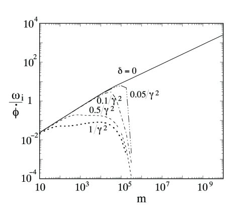
Figure 2: Growth rates as a function of azimuthal mode $m$ for $\zeta=0.02$, $\gamma=30$ and various energy spreads.

V Results and Discussion

In order for the growth rate to vanish the expression inside the root must be real and non-negative. Using our approximations for the Bessel functions it is seen immediately that the former condition is satisfied if $m>m_{2}$. This explains why the drop off occurs at $m=m_{2}$ regardless of the value of $\delta$ as long as the remaining real part is positive. This is the case if the field reversal parameter does not exceed the critical threshold

$$\zeta>m\gamma\delta^{2}~{}.$$ (44)

If the last inequality is not satisfied complex roots can only exist if $Z$ is complex which is the case for $m<m_{2}$. If however this inequality is satisfied the expression inside the root becomes negative for $m>m_{2}$ and an unstable solution exists, but the sharp cut-off is replaced by Eq. 44.

As discussed in the last section the azimuthal mode number $m$ resulting in the largest growth rate is either given by $m=2\gamma^{3}$ or $m=\zeta\gamma^{-1}\delta^{-2}$ whatever is greater. This guarantees that $(\Delta\tilde{\omega})^{2}$ is either still complex or real and negative with both leading to an unstable mode. For our allowed parameter range $2\gamma^{3}$ is typically larger. Thus,

$$\Im(\omega)\leq 2^{2/3}\dot{\phi}\gamma\sqrt{\zeta}\sim\gamma^{-1/2}\omega_{p}$$ (45)

where $\omega_{p}$ is the nonrelativistic plasma frequency.

Finally, let us consider small values of the azimuthal mode number $m$. So far we have have approximated the Bessel functions by Airy functions which makes them easier to compute especially for large orders. For small $m$ this approximation cannot be justified and the Bessel functions have to be retained. In Figure 3 we solved the dispersion relation in the small $m$ regime. Also, their arguments depend on $\Delta\tilde{\omega}$ since $m<m_{1}$. An accurate calculation of the growth rates of modes with azimuthal mode nubers $m$ is important for the determination of the total power radiated, because the latter decreases with increasing $m$. Even for $m=1$ Eq. 39 and 40 give excellent results, presumably because the argument of the Bessel functions is close to their order for $\gamma\gg 1$ and $Z$ is independent of $w$ if $|w|^{2}=\left|\left(\frac{m}{2}\right)^{2/3}\left[\gamma^{-2}-2\Delta\tilde{\omega}-2(\xi-1)\right]\right|^{2}\ll 1$. The latter condition may be satisfied even if $|\Delta\tilde{\omega}|$ violates our assumption $|\Delta\tilde{\omega}|\ll\gamma^{-2}$.

Looking at Eq. 36 we conclude that the quenching of the instability, i.e. the existence of the additional $\delta^{2}$ term in the denominator, is due to both the non-zero thickness of the layer and $\Omega^{\prime}\neq 0$. However, it is important to note that the instability relies on the negative mass effect and would not exist in the absence of shear in our model.

Figure 3: Growth rates as a function of azimuthal mode $m$ for $\zeta=0.02$, $\gamma=30$ and various energy spreads. The Bessel functions were retained in order to compute the growth rates in the low $m$ regime correctly.

Appendix A Green’s Function

The Green’s function for the potentials give

$$\delta\Phi({\bf r},t)=\int dt^{\prime}d^{3}r^{\prime}~{}G({\bf r}-{\bf r^{\prime}},t-t^{\prime})~{}\delta\rho({\bf r}^{\prime},t^{\prime})~{}.$$

$$\delta{\bf A}({\bf r},t)=\int dt^{\prime}d^{3}r^{\prime}~{}G({\bf r}-{\bf r^{\prime}},t-t^{\prime})~{}\delta{\bf J}({\bf r}^{\prime},t^{\prime})~{},$$ (46)

where

$$\left(\nabla^{2}-{\partial^{2}\over\partial t^{2}}\right)G({\bf r},t)=-4\pi\delta(t)\delta({\bf r})~{},~{}~{}\tilde{G}({\bf k},\omega)={4\pi\over{\bf k}^{2}-\omega^{2}}~{},$$

$$G({\bf r},t)=4\pi\int_{C}d\omega\int d^{3}k~{}{\exp(i{\bf k\cdot r}-i\omega t)\over{\bf k}^{2}-\omega^{2}}~{},$$ (47)

where $\tilde{G}$ is the Fourier transform of the Green’s function. The “C” on the integral indicates an $\omega-$integration parallel to but above the real axis, ${\rm Im}(\omega)>0$, so as to give the retarded Green’s function.

Because of the assumed dependences of Eq. (5), we have for the electric potential,

$$\delta\Phi_{\omega mk_{z}}(r)=2\int_{0}^{\infty}r^{\prime}dr^{\prime}\int_{0}^{\infty}\kappa d\kappa\int_{0}^{2\pi}d\alpha~{}~{}\delta\rho_{\omega mk_{z}}(r^{\prime})\big{[}..\big{]}$$

$$=4\pi\int_{0}^{\infty}r^{\prime}dr^{\prime}\int_{0}^{\infty}\kappa d\kappa~{}{J_{m}(\kappa r)J_{m}(\kappa r^{\prime})\over\kappa^{2}-(\omega^{2}-k_{z}^{2})}~{}\delta\rho_{\omega mk_{z}}(r^{\prime})~{},$$ (48)

where

$$\big{[}..\big{]}\equiv{\exp(im\alpha)J_{0}\{\kappa[r^{2}+(r^{\prime})^{2}-2rr^{\prime}\cos\alpha]^{1/2}\}\over\kappa^{2}-(\omega^{2}-k_{z}^{2})}~{},$$

where $\kappa^{2}\equiv k_{x}^{2}+k_{y}^{2}$. Because $\omega$ has a positive imaginary part, this solution corresponds to the retarded field. Also because ${\rm Im}(\omega)>0$, the $\kappa-$integration can be done by a contour integration as discussed in Watson1966 which gives

$$\delta\Phi_{\omega mk_{z}}(r)\!=\!2\pi^{2}i\int_{0}^{\infty}\!\!\!r^{\prime}dr^{\prime}J_{m}(kr_{<})H_{m}^{(1)}(kr_{>})\delta\rho_{\omega mk_{z}}(r^{\prime}),$$ (49)

where $k\equiv(\omega^{2}-k_{z}^{2})^{1/2}$, where $r_{<}$ ($r_{>}$) is the lesser (greater) of $(r,r^{\prime})$, and where $H_{m}^{(1)}(x)=J_{m}(x)+iY_{m}(x)$ is the Hankel function of the first kind. Because $(\delta A_{\phi},\delta J_{\phi})=-(\delta A_{x},\delta J_{x})\cos\phi+(\delta A_{y},\delta J_{y})\sin\phi$, we have instead of Eq. (49),

$$\delta\Psi^{\omega mk_{z}}(r)=r\delta A_{\phi}^{\omega mk_{z}}=\pi^{2}ri\int_{0}^{\infty}\!\!\!r^{\prime}dr^{\prime}\delta J_{\phi}^{\omega mk_{z}}(r^{\prime})$$

$$\cdot J_{m+1}(kr_{<})H_{m+1}^{(1)}(kr_{>})+J_{m-1}(kr_{<})H_{m-1}^{(1)}(kr_{>}).$$ (50)

For $m\gg 1$, one can show that in this equation $[J_{m+1}H_{m+1}^{(1)}+J_{m-1}H_{m-1}^{(1)}]/2=J_{m}H_{m}^{(1)}$ to a good approximation. Equations (49) and (50) are useful in subsequent calculations.

References

• Manchester & Taylor (1977) Manchester, R.N., & Taylor, J.H. 1977, Pulsars, (Freeman & Co.: San Francisco)
• (2) G.ย Benford and D.ย Tzach, Ap&SS 80, 307 (1981)
• (3) B.ย S.ย Schmekel, R.ย V.ย E.ย Lovelace, and I.ย M.ย Wasserman, Phys. Rev. E 71, 046502 (2005)
• (4) J.ย Arons and D.ย F.ย Smith, ApJ 229, 728-733 (1979)
• (5) R.ย C.ย Davidson, Physics of Nonneutral Plasmas, (Imperial College Press, London 2001)
• (6) B.ย S.ย Schmekel, Phys. Rev. E 72, 026410 (2005)
• (7) P.ย Goldreich and D.ย A.ย Keeley, ApJ 170, 463 (1971)
• (8) R.ย Buschauer and G.ย Benford, Mon. Not. R. astr. Soc. 185, 493 (1978)
• (9) C.ย E.ย Nielson, A.ย M.ย Sessler and K.ย R.ย Symon, Proc. of International Conference on High Energy Accelerators and Instrumentation, pp. 239, (CERN, Geneva, 1959)
• (10) A.ย C.ย Entis and A.ย A.ย Garren and L.ย Smith, Proceedings of the 1971 Particle Accelerator Conference, pp. 1092-1096, (IEEE, Piscataway, New Jersey, 1971)
• (11) R.ย J.ย Briggs and V.ย K.ย Neil, Plasma Physics, 9, 209-227 (1967)
• (12) A.ย A.ย Kolomenskii and A.ย N.ย Lebedev, Proc. of International Conference on High Energy Accelerators and Instrumentation, pp. 115, (CERN, Geneva, 1959)
• (13) S.ย Heifets and G.ย Stupakov, Phys. Rev. ST Accel. Beams 5, 054402 (2002)
• (14) O.ย Larroche and R.ย Pellat, Phys. Rev. Lett. 59, 1104 (1987)
• (15) R.ย V.ย E.ย Lovelace and R.ย G.ย Hohlfeld, ApJ 221, 51 (1978)
• (16) G.ย N.ย Watson, A Treatise on the Theory of Bessel Functions, pp. 428-429, (Cambridge University Press, Cambridge, 1966)