Radioelectric field features of extensive air showers observed with CODALEMA

Abstract

Based on a new approach to the detection of radio transients associated with extensive air showers induced by ultra high energy cosmic rays, the experimental apparatus CODALEMA is in operation, measuring about 1 event per day corresponding to an energy threshold $\sim 5\times 10^{16}$ eV. Its performance makes possible for the first time the study of radio-signal features on an event-by-event basis. The sampling of the magnitude of the electric field along a 600 meters axis is analyzed. It shows that the electric field lateral spread is around 250 m (FWHM). The possibility to determine with radio both arrival directions and shower core positions is discussed.

1 Introduction

Radio emission associated with the development of Extensive Air Showers (EAS) was investigated in the 1960’s [1, 2]. A flurry of experiments provided initial information about signals from $10^{17}$ eV cosmic rays [3], but plagued by difficulties (poor reproducibility, atmospheric effects, technical limitations) efforts almost ceased in the late 1970’s while ground particle [4] and fluorescence [5] detector work continued. With the growing interest for ultra high-energy cosmic ray (UHECR) research involving giant surface detectors [6], radio detection however appears as a promising tool for future apparatus considering its specific advantages: low-cost, high duty cycle and sensitivity to the longitudinal development of the showers. Although the rebirth of radio pulse investigation [7, 8, 9, 10, 11] is recent, first available results [12, 13] demonstrate the feasibility of EAS radio detection.

The CODALEMA (COsmic ray Detection Array with Logarithmic Electro-Magnetic Antennas) experiment, located at the Nançay radio observatory [14], is a part of this new effort. Its originality lies in completely recording the form of the transient radio signals together with sampling the electric field over a few hundred meters range on the ground. This makes possible both the determination of arrival times and directions of radio pulses and the study of their field amplitude impact parameter dependences. The measurement of UHECR around $10^{20}$ eV is the admitted goal of such experimental development, but a proof-of-principle demonstration at such a large energy would suffer from a lack of statistics without an extensive antenna array. This point can be circumvented in a first stage by working around $10^{17}$ eV where a measurable signal amplitude [3, 15] is expected at not too large distances from the shower core. Considering a vertical shower falling upon the detector, the predicted transient should reach 150 $\mu$V/m with a 10 ns FWHM duration for $10^{17}$ eV cosmic rays [3, 7, 13]. Transposed in the frequency domain, the corresponding pulse spectrum should extend from 1 to 100 MHz. Thus, with a wide band antenna it should be possible to recover the original pulse shape, allowing for energy determination and providing information on the nature of the primary particle with minimal assumptions concerning its electromagnetic shower- signature. The design of CODALEMA is based on these expectations.

CODALEMA has already provided firm evidence for a radio emission counterpart of EAS with an estimated energy threshold of $5\times 10^{16}$ eV [13]. In the present paper, we extend the characterization of EAS candidates giving special attention to the electric field pattern observed on an event-by-event basis. The experimental set-up is described in section 2 and general event properties are given in section 3. The selection of EAS radio candidates is discussed in section 4. Section 5 is the central part of the present study and details first observations on EAS electric field lateral distributions from a few illustrative examples. Section 6 discusses frequency dependences. Some conclusions are given in section 7.

2 The CODALEMA experiment

The technical characteristics of the detector along with detection and analysis methods have been extensively described in Ref. [13]. As shown in Fig. 1, the set-up uses 11 log-periodic antennas of the Nançay Decameter Array DAM [14] and 4 particle detectors originally designed as prototypes for the Pierre Auger Observatory [16]. Four of the antennas, namely NE, SE, SW and NW, are located at the corners of the Decameter Array (a rectangle of 87 m$\times$83 m). In order to investigate the electric field spread, the main improvement, as compared to the previous apparatus [13], lies in the instrumentation of an East-West line, 608 m long, 40 m South of the SW-SE antenna axis. This long baseline is equipped with 7 antennas with a sampling interval of 87 m from L1 to L5 and L2 to L6 and 130 m for L0, L1 and L2.

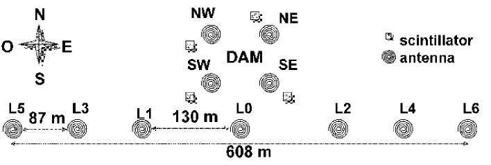
Figure 1: Current CODALEMA set-up. The particle detectors (scintillators) act as a trigger with a fourfold coincidence requirement. The 608 m long baseline in the East-West direction makes possible measurements of the electric field profile.

All the antennas are linked, after radio frequency (RF) signal wide band amplification (35 dB), via low loss coaxial cables (SUHNER S12272-04) to LeCroy digital oscilloscopes (8 bit ADC, 500 MHz sampling frequency, 10 ${\mu}$s recording time). To get enough sensitivity to fast transients with these ADCs, the antennas are band-pass filtered ($24-82$ MHz) so that the ADCs are not required to handle large amplitude, low-frequency interference.

Each 2.3 m² particle detector module (station) has two layers of acrylic scintillator, read out by a photomultiplier located at the centre of each sheet. The photomultipliers have copper housings and it has been verified [13] that no correlation exists between individual photomultiplier signals and the presence of antenna signals. The coincidence between the top and bottom layers is obtained within a 60 ns time interval with a counting rate of 200 Hz per station. The whole experiment is triggered by a fourfold coincidence from the stations in a 600 ns time window. The corresponding counting rate is around 0.7 events per minute.

3 General properties of the recorded events

The directions of the particle showers are determined by triangulation, using arrival times from the digitized photomultiplier signals and assuming the particle wavefront is a plane. The angular acceptance of the trigger device can be studied by calculating its counting rate as a function of the zenith angle $\theta$ (see Fig. 2). A satisfactory description of the data is obtained using a $2\pi\,\sin\theta\,\cos^{2}\theta$ behavior multiplied by a Fermi-Dirac function (solid curve in Fig. 2). The latter contribution takes into account the extinction at the detector location of large zenith angle EAS [17]. Thus, the effective sky coverage extends up to $60^{\circ}-70^{\circ}$ zenith angles. In addition, the azimuthal angle distribution behaves as expected for our set-up. The absence of anomalies in these distributions leads us to conclude that satisfactory performance is achieved for triggering the radio array.

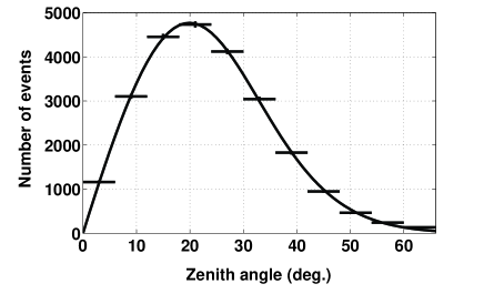
Figure 2: Cosmic ray counting rate measured during 2314 hours as a function of the zenith angle. The fall-off observed at low elevation is related to the decrease of the effective size of the array and detectors as well as to an increase of the detection energy threshold for the most inclined showers.

For each fourfold coincidence from the particle detectors, the 11 antenna signals are recorded. Due to the relatively low energy threshold, only a small fraction of these air shower events is expected to be accompanied by significant radio signals. Recognition of radio transients is made by offline analysis using first a 37-70 MHz digital filter. The maximum voltage is then searched for in a 2 $\mu$s wide time window correlated to the trigger time. The average noise and its standard deviation are calculated, for each antenna and each event, in a 7.2 $\mu$s wide time window out of the signal one. More details about the resulting signal determination and the corresponding threshold criterion based on the individual event noise can be found in Ref. [13]. When at least 3 antennas are flagged, a triangulation procedure calculates the arrival direction of the radio wave using a plane wavefront assumption. At this level of selection, the counting rate of these 3-antenna events is about 1 event every 2 hours.

The capability of the radio antenna device to reconstruct signal directions by such triangulation is illustrated by Fig. 3. It shows the distribution of the arrival directions of events after the trigger process described above. A substantial number of events comes from directions near the horizon and exhibit broad accumulations at a few azimuth values. They correspond to Radio Frequency Interference (RFI) events and the selection discussed in the next section eliminates them. The remaining EAS candidates turn out to be randomly distributed in the sky and have zenith angles below 60^∘ (as expected from trigger bias). Assuming spherical wave propagation, most of the RFI were found to originate from electrical devices located in the near environment of the Nançay observatory site. Specific runs with a trigger generated by the antennas have been performed and described in Ref. [13]. They showed that a part of the localized sources can emit transients at specific and restricted time sequences, in contrast to the expected random behavior of EAS events. For example, the group of events located around an azimuthal angle of 190^∘ results from the rotating device of the primary mirror of the Nancay Decimetric radiotelescope which generates events at well identified time sequences.

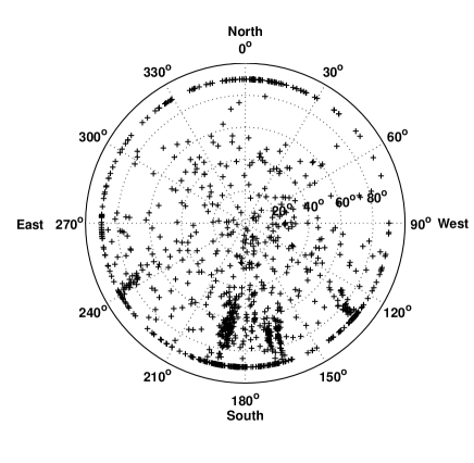
Figure 3: Sky map of the reconstructed directions of 1151 radio coincidences ($\geq$ 3-antennas) recorded by CODALEMA over 96 days and triggered by four-fold coincidences on particle detectors. Dotted internal circles refer to indicated values of zenith angles up to the horizon; the external values stand for azimuthal angles.

4 Direction and timing properties of the EAS radio events

Our characterization of EAS radio signals starts by comparing arrival times and incident directions as determined by the antenna array on the one hand, and the particle detector array on the other hand. The radio wave arrival time at any particular location is first extracted from off-line triangulation of multi-antenna events. The corresponding time distribution can then be compared with the particle front time reference supplied by the scintillator signals. The time difference distribution obtained by this procedure is shown in Fig. 4. A sharp peak, a few tens of nanoseconds wide, is clearly visible, showing an unambiguous correlation between some radio events and particle triggers. Outside of the coincidence peak, the flat distribution corresponds to accidental radio transients which are not associated with air showers but which randomly occurred in the 2 $\mu$s window where the search is conducted as described in section 3. Being uncorrelated to the particles, these events have a uniform arrival time distribution. EAS candidates are those for which the arrival time difference between the two detector systems satisfies the relation $0\leq\Delta t\leq 100$ ns, corresponding to the peak in Fig. 4.

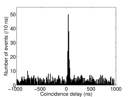
Figure 4: Distribution of time delays between the radio plane front and the particle plane front. The time of passage of the radio wavefront through a reference point, chosen as the centre of the triangle formed by SW, SE, L0 antennas, is compared, for all events, to that of the particle front. The distribution exhibits a sharp peak corresponding to EAS candidates.

If the time-correlated events actually correspond to EAS, the arrival directions reconstructed from both scintillator and antenna data should be close to each other. Fig. 5, left-hand side, shows the distribution of the angle between the two reconstructed directions, without the time cut (grey histogram) and with a time cut of $0\leq\Delta t\leq 100$ ns around the peak displayed in Fig. 4 (black histogram). When selecting candidates in the peak, some chance events remain and can be clearly identified by plotting the angular difference distribution between radio pulses and particles. Most of the chance events have a large angular difference value and therefore true radio-particle coincidences can be selected using a small-angle cut on this distribution. Fig. 5, right-hand side, shows that the EAS event angular differences fit a Gaussian distribution, centered at zero degrees and multiplied by a sine function coming from the solid angle factor. The standard deviation of the corresponding Gaussian is about 4 degrees. This value combines particle detector and antenna reconstruction accuracies. Based on the gaussian fit, the cutoff in angular difference for true radio-particle coincidences can be set to 15^∘. From the shape of the chance event distribution seen in Fig. 5-left between 15^∘ and 100^∘ the expected number of chance events below 15 ^∘ is 15.

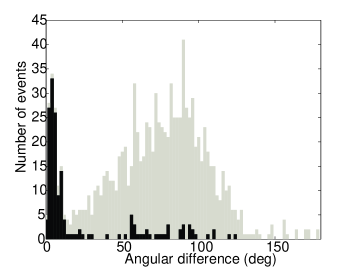
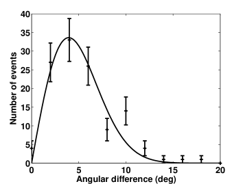
Figure 5: Left: Distribution of relative angles between particles and radio-pulses without time cut (grey histogram) and with a time cut around the coincident peak of the time difference distribution (black histogram). Right: Distribution of angular difference after time cutting around the coincident peak, fitted by an analytical expression of the expected angular dependence. Error bars are calculated as the square root of the number of events in each bin.

Recognition of chance events in the time-coincidence peak of Fig. 4 can be performed taking advantage of the angular difference distribution of Fig. 5: a third of the events (52 out of 164) in the time-coincidence peak have angular differences greater than 15^∘ and can thus be removed. Thus, 112 events remain as true EAS coincidences, while the chance event number (15) in the angular range $\theta=0:15^{\circ}$ results in $(1/20)\times 15=0.75$ count after both time and angular coincidence cuts. The corresponding signal directions, reconstructed as explained in section 3, are displayed in Fig. 6. The rate of chance coincidences eliminated in this way (52 in 100 ns) is fully compatible with the observed uniform distribution in the 2 $\mu$s window (about 5 every 10 ns). As already mentioned, these chance events occur mostly from directions close to the horizon, as shown in Fig. 3, and are typically from RFI due to human activities or from distant thunderstorms. As will be seen in the next section, these events are characterized by an almost uniform electric field amplitude, at least on the distance scale of our apparatus.

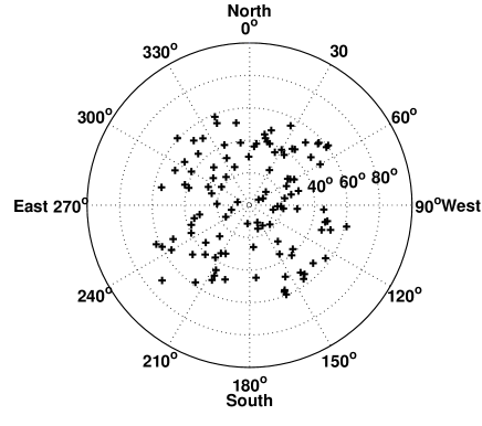
Figure 6: Sky map of the reconstructed directions of 112 air-showers coincidences recorded over 96 days by CODALEMA, triggered by four-fold coincidences on particle detectors and after time and angular cuts as explained in the text. Angular coordinates as in Fig. 3.

In order to study the radio detection performance on confirmed EAS, the particle detector and radio detector acceptances have been compared as a function of the zenith angle (see Fig. 7) and of the azimuthal angle. This procedure should also bring to light possible detection inefficiency due to antenna lobe acceptance effects. In this study, only the subset of true radio coincidences (events present in the peak of the time distribution satisfying the above 15^∘ angular criterion) were taken into account. Although antennas of the Decameter Array, initially dedicated to the observation of the Sun and Jupiter, are tilted $20^{\circ}$ to the south, the azimuthal distribution indicates that the antenna array does not present a markedly higher sensitivity for signals coming from the south. (As previously noted, the particle detector selects EAS with zenith angle smaller than about 60^∘, see Fig. 2.) As a function of zenith angle, a higher acceptance ratio (a factor about 50 within statistics) is observed at low elevation angles. A substantial contribution to this evolution is coming from the fall-off of the trigger device efficiency at large angle, due to simple geometrical effects and increase of the energy threshold (see discussion of Fig. 2 in section 3). As a matter of fact, the gross trend of the compared acceptances can be reproduced ignoring any non trivial zenith dependence originating from the antennas. More precisely, the antenna gain pattern has an attenuation of less than 2 dB in the range $\theta\leq 60^{\circ}$. This highlights the specific and unique advantage of a radio antenna network for the observation of inclined showers. A more detailed and quantitative statement must take into account several dependences such as those of the electromagnetic signal with impact parameter [18], the yield evolution in larger atmospheric densities encountered by inclined showers and the energy dependence of the antenna multiplicity. The scope of the next section, which will present the analysis of field patterns, is to bring some new valuable pieces of information regarding those dependences.

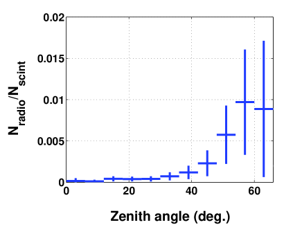
Figure 7: Counting rate ratio of multi-antenna events to the trigger events versus zenith angle showing the comparative acceptance of the two detectors.

To summarize, from 2314 hours data taking, 1151 coincidences (with at least $\geq$ 3-antennas) were observed in the 2 $\mu$s trigger coincidence time-window containing 112 true EAS and 52 chance coincidence events as determined by a time cut of $0\leq\Delta t\leq 100$ ns around the peak of arrival time difference between the two types of detectors and a cutoff at 15^∘ in their angular difference. After application of our selection procedure, the resulting counting rate of EAS events with a radio signal counterpart is close to 1 per day. The physical characteristics of the electromagnetic field spread associated with these radio EAS radio events will be now considered.

5 Electric field topologies of the EAS radio events

With our limited size antenna array, the number of tagged antennas per event is highly variable, depending on the shower energy, core position and zenith angle. Nevertheless, each tagged antenna provides a measured voltage associated with a particular geographical location. Thus a sampling of the electric field amplitude over the area covered by the antenna array is possible on an event-by-event basis.

For this purpose, antenna cross-calibration has to be checked. This is discussed in the Appendix where it is shown that antenna responses are identical, with differences at the level of a few percent. Conversion from ADC voltage to electric field magnitude is explained in Ref. [13].

Fig. 8 shows a sample EAS event with an 11-antenna multiplicity. The signal amplitude from each antenna is represented by the area of the gray circle. The arrival direction has been reconstructed from both scintillator and antenna data (a difference of 1.6^∘ is found between the two estimations for this event) and indicates that it corresponds to a shower with a zenith angle of 51^∘ and an azimuthal angle of 350^∘.

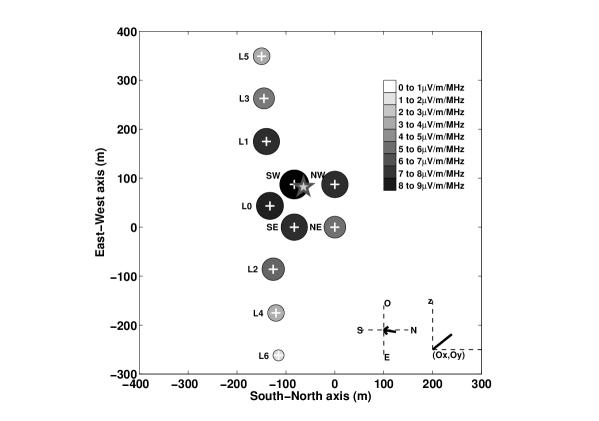
Figure 8: Footprint of a transient EAS event on the CODALEMA set-up. Crosses correspond to positions of each individual antenna, the gray-shaded circular area being proportional to the indicated measured electric field. The arrival direction and elevation angle of the event are shown in the bottom right corner. The star, near antenna SW for this event, indicates the shower core location reconstructed from the barycentre of the two distributions plotted in Fig. 9.

The electric field distributions for this EAS event (squares) are shown in Fig. 9, for the East-West (left-hand side) and South-North (right-hand side) antenna axis, together with a chance event (triangles). The chance event has been identified using the procedure described in section 4 and belongs to a set of events identified as resulting from a particular RFI source (corresponding to one of the accumulations in Fig. 3). Circles indicate the threshold level as determined by the procedure mentioned in section 3. Fig. 9 shows that the topologies are clearly different between EAS and RFI events. The RFI event (triangles) displays an electric field with a quasi uniform amplitude. This behavior corresponds to what is expected for a distant source. To the contrary, EAS candidates falling in the vicinity of the array should present a quite different electric field behavior [15]. Indeed, the EAS event (squares) shows a large field amplitude variation depending on the position of the antenna with respect to the shower axis. An estimation of the location of the shower impact can be derived from the position of the barycentre. It is indicated by a star in Fig. 8.

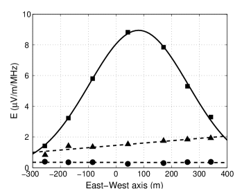
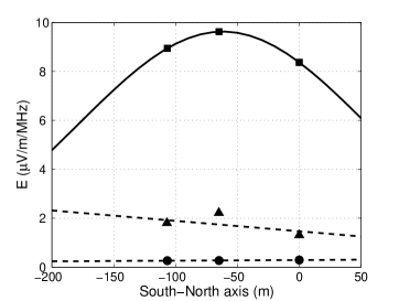
Figure 9: Electric field variations recorded on different antennas for an EAS event (squares, full line) and an anthropic transient (triangles, dashed line). Circles indicate threshold levels. Lines between data points are just a guide for the eye. Left: Antennas along the East-West line direction. Right: South-North direction (antennas L0,SW,NW).

The electric field values can be compared with the galactic noise level [3]. Following the definition of Ref. [9]

$$E^{\mathrm{sky}}(\mu\mathrm{V/m/MHz})=\sqrt{20/g}\times\sqrt{\Delta t(\mu\mathrm{s})},\ \mathrm{at}\ 55~{}\mathrm{MHz,}$$

where $g$ is the antenna gain ($g=5$) and $\Delta t$ is the integration time. The occurence of $\Delta t$ is because we define an electric field per unit bandwidth (related to the square root of an energy spectral density), a quantity relevant to the description of a finite time signal (such as EAS electric field), whereas the sky background is a steady signal for which power spectral density is more appropriate. Thus, the conversion energy$=\Delta t\times$power. For $\Delta t=1~{}\mu$s, $E^{\mathrm{sky}}=2\mu$V$/$m$/$MHz. For pulses of duration smaller than $1~{}\mu$s, as is the case of the EAS transients observed in CODALEMA, it is possible to reduce $\Delta t$, hence increasing the signal-to-noise ratio. In such a way, electric field as small as $1\mu$V$/$m$/$MHz could be observed in the present analysis.

The electric field maximum in both sampling directions can only be obtained for the subset of showers falling inside the area delimited by the four corners of our antenna array. The present set-up is limited in this respect due to the small extent of the array along the South-North direction. In order to gauge the extension of the area illuminated by the radio component of EAS, the electric field distribution has been studied along the East-West axis without any constraint along the South-North line. Field patterns for four typical radio EAS events (out of 64  with antenna multiplicity $\geq 4$) are presented in Fig. 10. EAS events show a large variation of field amplitudes depending on the position on the E-W axis. The differences from one event to the other are the consequence of several geometrical (direction, impact location) and physical (energy, depth at maximum) sources of variation in the EAS. They cannot be disentangled using the present experimental set-up but the patterns shown in Fig. 10 can be exploited by themselves for the determination of the shower impact. Lines, drawn in Fig. 10 for this purpose, are the result of a calculation which will be explained later.

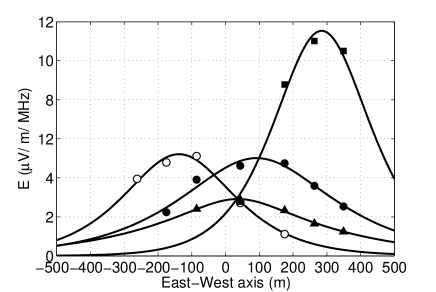
Figure 10: Electric field variations recorded on the different antennas in the East-West direction for four EAS events (squares). The full lines result from the exponential fits discussed in the text.

The characteristic shape of the field distribution is one genuine signature of EAS radio events. It may help to discriminate them from RFI events and may thus be used as an important criterion of selection in a stand-alone radio experiment. More thorough investigations are certainly needed to establish this possibility. The present observations corroborate the earlier campaigns of experiments performed in a self triggering mode [13] where the possibility of reconstruction of event waveforms and directions has been demonstrated. The occurrence of accidental (anthropic) close sources of emission can be fairly well handled using specific prints like trajectory reconstruction, field distribution or time evolution. So far, the distributions shown in Fig. 10 demonstrate that EAS electric-field measurements are feasible over distances at least as large as 600 m and presumably up to 1 km. Such values should be associated with the most energetic events recorded at our site which, based on their rate, are in the range of 1–5$\times 10^{17}$ eV.

The electric field variation in the antenna-based coordinate system depends on the arrival direction, in particular on the zenith angle. This makes comparisons between different showers or between the E-W and S-N axis difficult. For this purpose, it is thus preferable to reformulate the lateral dependence of the electric field profile (EFP) in a shower-based coordinate system, obtaining the shower axis orientation from the reconstructed arrival direction. To carry out this analysis an exponential profile fit $E(d)=E_{0}\times\exp(-d/d_{0})$ has been used where $d$ is the distance between the shower axis and each fired antenna in the event considered. This form corresponds to the radio data fit discussed by Allan [3]. This particular form has a minimal number of free parameters $E_{0}$, $d_{0}$, and the E-W and S-N coordinates of the impact point on the ground. To initiate the 4-parameter fit, the core position of the shower is first roughly estimated by a barycentre calculation of the amplitudes on both the South-North and East-West axis of the array.

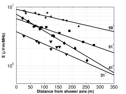
Figure 11: Electric field profiles (EFP) on a logarithmic scale for a set of radio EAS events recorded on CODALEMA. The measured amplitude in $\mu$V/m/MHz is plotted versus the distance from the antenna to the shower axis (in meters). The associated reconstructed zenith angle is indicated on each plot. Both amplitude and slope of the fitted exponential law are variable parameters from one event to the other.

Illustrative EFPs from another sample of antenna events with multiplicity $\geq 4$ are given in Fig. 11. According to the signal threshold criteria described in section 3, for events where one (or several) antenna is not flagged, only upper limits are used, based on the threshold level. Data appear to be well fitted by the above exponential law (full lines) from a few tens to several hundred meters. As expected, the slope and amplitude parameters are variable from one event to the other. Extrapolations of the electric field at the locations of the shower cores could reach values as large as 10 $\mu$V/m/MHz during the data taking here discussed. Using the E-W and S-N coordinates of the impact point thus determined as fit parameters, the field values obtained with such fits can also be compared to the data field values sampled in the ground coordinate system shown in Fig. 10. This is illustrated by full lines in this plot. Data and maxima positions are very well reproduced by this parameterization. In addition to the consistency of the exponential law hypothesis with the shower observables, this also demonstrates the feasibility of a shower impact determination based only on an investigation of the electric field pattern over a limited geometry of antennas.

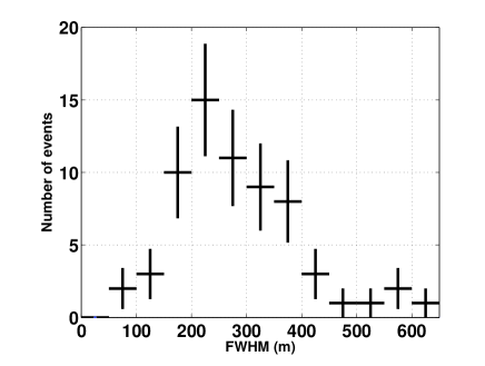
Figure 12: Distribution of the electric field FWHM extent, in meters, for the reconstructed events with antenna multiplicity $\geq 4$.

The electric field width distribution (the FWHM of the exponential) is presented in Fig. 12 for the subset of $64$ events selected from true EAS with multiplicity $\geq 4$. The mean extension of the field is found to be around 250 m FWHM. This result may constitute a first step toward the determination of the antenna spacing for the design of a large radio array. In contrast to standard measurements by ground particle detector arrays, from which a density profile can also be extracted, we note that radio antennas are sensitive to the overall shower development making the measurement almost free of any particle number fluctuations.

A dependence of the electric field amplitude on the energy and the nature of the primary particle is clearly expected [3, 15] but little data is available [3, 12]. In the same way, the slope of the exponential fit should vary with the shower zenith angle. To our knowledge, no such simple correlations have been measured yet. A greater amount of data is obviously needed as well as a much larger detector array in order to go further into the physical analysis with some statistical significance.

As long as the maximum of the field distribution is observed along one of the sampling axis, indications of core positions can be extracted, even if they lie outside the active area delimited by the antennas. Core locations extracted from the exponential fits are shown in Fig. 13 for the subset of $64$ events above defined. From the examination of the quality of the fits obtained for the profiles (see examples in Fig. 10 and 11), we estimate the uncertainty on the E-W position ($y_{0}$) around 10 m for the strongest radio events falling close to the array centre. The uncertainty on the S-N position ($x_{0}$) is somewhat larger. A variation of $y_{0}$ by 10 m results in a variation of the parameter $d_{0}$ by about $10\%$ to produce a fit of comparable quality. This reflects the correlation between the different parameters. Fig. 13 shows that more core locations are found in the vicinity of the trigger particle detector array as expected. Far from the centre, the density of impacts is small and the precision on core locations and correlations with the arrangement of antennas and particle detectors require further investigation. The present work shows the possibility to use field profile studies for core position determinations. Inherent limitations with the restricted set-up geometry presently used foster the future extension of our antenna set-up, particularly along S-N line, for core determination purposes. An upgrade of the particle detector array will allow useful comparison and correlation studies.

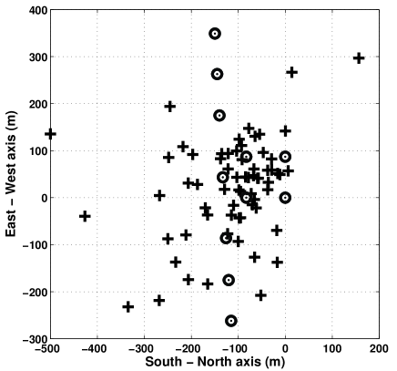
Figure 13: Core positions calculated for the complete subset of true EAS events with antena multiplicity $\geq 4$. Each cross corresponds to a reconstructed shower core position. Circles correspond to the positions of antennas.

6 Frequency dependence

Another aspect which can be studied on an event-by-event basis is the frequency dependence of the electric field spectrum, and taking advantage of the size of the EW line, it is also possible to see how the spectrum evolves with the distance of the antenna location to the shower axis.

The general feature observed in the 30–70 MHz frequency range is a powerlaw fall-off of the voltage with frequency. Hence significant data for the whole frequency range are only available for the strongest events. If in addition it is required that at least one antenna is close ($d\leq 50$ m) and one is distant ($d\geq 200$ m), we are left with only 3 events to consider. The discussion below should thus be considered as a foretaste of what could be achieved with a larger statistics, or if the frequency range could be extended downwards, below 30 MHz.

The analysis consists in selecting, for each antenna signal in a given event, a window of 256 points surrounding the radio pulse (time signal) and 16 distinct windows of 256 points each outside the signal window (background). Then, Fourier transforms of both sets are calculated in order to select those pulses that have their spectra well above the noise spectrum. The latter is estimated as the average spectral amplitude over the 16 background windows. Fig. 14 shows an example of such a comparison. The fall-off in the range 30–70 MHz can be reasonably well described by a power-law $V_{\nu}=K\times\nu^{-a}$ in which $a$ can be estimated on each signal. For this purpose, only frequencies in the range 30–70 MHz are retained under the condition that the signal amplitude spectrum exceeds four times that of the background. We then performed a least square log-log fit of the signals having at least 10 frequency points fulfilling the above criterion.

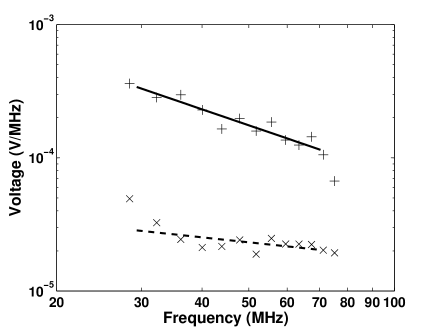
Figure 14: Voltage spectra and simple least square fits of both the signal ($+$) and the background ($\times$).

An example of spectral index dependence on distance is shown in Fig. 15 for the electric field ($E_{\nu}\propto\nu\times V_{\nu}$). For the small event set where such a study could be performed, we found good descriptions of the signal spectra with the power-law fall-off $E_{\nu}=K\times\nu^{1-a}$ with $1-a$ ranging from $-1.5$ to sligthly below 0. Confidence interval on $a$ is about $0.2$. The variation with distance is only mild if any.

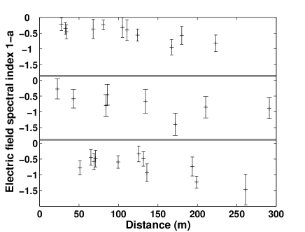
Figure 15: $1-a$ vs shower-antenna distance (in meters) for three events. The three events shown are those which have both a close, $d\leq 50$ m, and a distant antenna, $d\geq 200$ m.

The data collected is too sparse to draw any conclusion. From the discussion in Ref. [3], the frequency spectrum should be constant in the MHz range and fall-off at larger frequencies as a consequence of the loss of coherence. The frequency cut-off and precise behaviour of the fall-off depend on the geometrical and physical characteristics of the shower and on the antenna location. For example, the time duration of the electric field pulse is expected to rise, and consequently the frequency cut-off is expected to decrease, when the impact parameter increases [3, 13]. It follows that a constant spectral index is not expected in the full frequency range but rather it should evolve from $1-a=0$ at small frequency to negative values beyond the frequency cut-off. The observed constancy of $1-a$ may then just reflect the too-limited accessible frequency range of the present study. The observed spectral index variation from one signal to the next may be attributed to the change of the coherence condition, in particular the frequency cut-off. Since the latter depends on the impact parameter [3], a more thorough study would be of great interest to complement the impact parameter evolution described in section 5.

7 Summary and outlook

Features of the electric field transients generated by more than a hundred extensive air shower events have been observed with CODALEMA. Through the evolution of this sample of events, the observed characteristics allow the determination of the EAS core location together with the electric field magnitude and spread, on an event-by-event basis using an electric field profile function. Electric field profiles show slopes and amplitudes which are variable between events. These patterns offer possibilities to discriminate between EAS events and radio frequency interferences. Frequency dependence of EAS electric field has been also observed. Such detailed electric field correlations or characteristics have been predicted to be related to important physical quantities such as the EAS energy, the nature of their primaries and various important shower evolution parameters [3, 15]. The present results show for the first time the feasability of such studies on an event-by-event basis using a radio detection set-up in combination with particle detectors. More complete works and higher statistics are clearly necessary to establish the exact nature of the physical correlations detectable by the measurements of the radioelectric field features.

In addition, the various sources that can influence the electric field distribution in a given event are hard to disentangle with the limited set-up described here. An upgrade with new particle detectors is already underway to provide more information on each event. They will give an independent determination of the core position and an estimate of the shower energy, invaluable information at the present stage of development of the radio technique.

It has been emphasized that the observed field pattern on the various antennas constitutes a clear “radio” signature. This suggests that it may be possible to discriminate an EAS event from a fortuitous one, using a self triggering array of radio antennas. This is one further step toward a stand-alone system that could be deployed over a large area or added to an existing surface detector such as the Pierre Auger Observatory. The radio signals could then provide complementary information about the longitudinal development of the shower, as well as the ability to lower the energy threshold. More data and technical upgrading are planned in order to examine the contribution that the radio detection method could bring to the determination of the energy and nature of ultra high energy cosmic rays.

The fact that inclined or horizontal radio waves could be efficiently detected with our set-up may be of great interest to EAS detection if the electric field patterns discussed in the present study turn out to allow for a clear discrimination between EAS radio events and other noise transients close to the horizon. Among various particles able to generate air showers, neutrinos are thought to probably be the only ones which could address the nature and source location of ultra energetic cosmic rays. Taking into account the sensitivity of the radio detection method to inclined extensive air showers [18], the presented results could considerably enlarge the scope of such studies for cosmology related phenomena.

Appendix A Antenna response comparison

Comparison of the antenna and associated electronics responses is done using the diurnal behavior of the ambient electric field in the frequency band of interest. The bulk of the radio data, which does not contain any transients, shows a steady variation of the electric field during the day, at the level of $\pm 10\%$, with identical time evolution from one antenna to the other. This electric field component can be considered as uniform over the antenna array and used as a common reference to check for antenna gain line up. The observed deviation is smaller than $0.5$ dB.

For each event, the time averaged power $\mu_{n\,j}=\langle P\rangle_{\mathrm{noise}\,j}$ is calculated on each antenna $j$ in the noise window of the 37-70 MHz filtered signal. If this component of the signal originates from a common source which distributes it over the whole antenna array, $\mu_{n\,j}$ will reflect the gain of the channel. Fig. 16 shows the distribution of $\mu_{n}$ for one antenna over 8 months. The distribution extends to large values attributed to sources emitting occasionally or intense solar phenomena. The peak at small values, displayed on a smaller scale in the inset, corresponds to background conditions where no coherent signal has been seen in the frequency spectra. In order to remove the large fluctuations, a cut is applied on the data to deal only with the subset of events belonging to the peak.

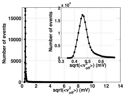
Figure 16: Distribution of $\sqrt{\mu_{n}}$ on antenna L1 over the full scale in mV. An accumulation is visible at small values. Higher excursions are due to occasional pollution incidents in the frequency band. The inset focuses on the peak that is of interest in our case as it corresponds to the absence of disturbances.

For every antenna, when plotting $\mu_{n}$ versus time over several months, the general trend of the variation from one event to the next is an oscillation with a period of one day. No correlation with the surrounding human activity is observed. This pattern, seen on every antenna with identical phased periodicity and deviation, should be associated to a single origin which can be considered as a source shining uniformly over the antenna array. Thus, having identified a common reference, relative gains can be compared. This is shown in Fig. 17 for the entire antenna array.

Calibration of each antenna using strong celestial radiosources is possible via interferometry using the full Decameter Array as a reference detector. This procedure is underway.

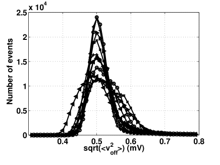
Figure 17: Distribution of $\sqrt{\mu_{n\,j}}$ in mV for the whole array.

References

- [1] G.A. Askar’yan, Soviet Phys. J.E.T.P. 14 (1962) 441.
- [2] T.C. Weekes, Proc. of the first int. workshop on “Radiodetection of high Energy Particle”, Los Angeles, November 16-18, 2000, AIP Conference Proceedings Vol 579 (2001) 3.
- [3] H.R. Allan, in: Progress in elementary particle and cosmic ray physics, ed. by J.G. Wilson and S.A. Wouthuysen (North Holland, 1971) 169.
- [4] N. Hayashida et al, Phys. Rev. Lett. 73 (1994) 3491; M. Takeda et al., Phys. Rev. Lett. 81 (1998) 1163.
- [5] D.J. Bird et al, Phys. Rev. Lett. 71 (1993) 3401; Astrophys. J. 441 (1995) 144.
- [6] Auger Collaboration, Nucl. Instrum. Meth. A 523 (2004) 50.
- [7] K. Green et al, Nucl. Instrum. Meth. A 498 (2003) 256.
- [8] A. Badea et al, Proceedings of CRIS2004, Nucl. Phys. Proc. Suppl. 136 (2004) 384.
- [9] H. Falcke, P. Gorham, Astropart. Phys. 19 (2003) 477.
- [10] D. Ardouin et al, Proceedings of the XXXIXth Rencontres de Moriond “Very High Energy Phenomena in the Universe”, La Thuile, Italy (2005) & astro-ph/0505442. Proceedings of the 29th ICRC, Pune, India (2005) & astro-ph/0507160. Proceedings of Rencontres de l’astrophysique française SF2A, Strasbourg, France (2005) & astro-ph/0510170.
- [11] I. Kravchenko et al, Recent results from the RICE experiment at the South Pole, astro-ph/0306408 (2003).
- [12] H. Falcke et al, Nature 435 (2005) 313, Letters to Editor.
- [13] D. Ardouin et al, Nucl. Instrum. Meth. A 555 (2005) 148.
- [14] A. Lecacheux, “The Nançay Decameter Array: a useful step towards giant, new generation radio telescopes for long wavelength radio astronomy”, in Radio Astronomy at Long Wavelengths, AGU monograph, 119 (2000) 321.
- [15] T. Huege and H. Falcke, Astropart. Phys. 24 (2005) 116.
- [16] M. Boratav et al., The AUGER Project: First Results from the Orsay Prototype Station, Proc. of the 24th ICRC, Rome, 954 (1995).
- [17] B. Revenu, private communication.
- [18] T. Gousset, O. Ravel and C. Roy, Astropart. Phys. 22 (2004) 103.