later
Statistical Algorithms for Identification of Astronomical X-Ray Sources
Abstract
Observations of present and future X-ray telescopes include a large number of serendipidious sources of unknown types. They are a rich source of knowledge about X-ray dominated astronomical objects, their distribution, and their evolution. The large number of these sources does not permit their individual spectroscopical follow-up and classification. Here we use Chandra Multi-Wavelength public data to investigate a number of statistical algorithms for classification of X-ray sources with optical imaging follow-up. We show that up to statistical uncertainties, each class of X-ray sources has specific photometric characteristics that can be used for its classification. We assess the relative and absolute performance of classification methods and measured features by comparing the behaviour of physical quantities for statistically classified objects with what is obtained from spectroscopy. We find that among methods we have studied, multi-dimensional probability distribution is the best for both classifying source type and redshift, but it needs a sufficiently large input (learning) data set. In absence of such data, a mixture of various methods can give a better final result. We discuss some of potential applications of the statistical classification and the enhancement of information obtained in this way. We also assess the effect of classification methods and input data set on the astronomical conclusions such as distribution and properties of X-ray selected sources.
keywords:
X-rays: general — methods: statistical — surveys1 Introduction
Since the launch of Chandra and XMM-Newton X-ray observatories at the end of 90’s our vision of the X-ray sky has been tremendously changed. The large collecting area of the XMM-Newton, and the sensitivity and high spatial resolution of Chandra ([van Speybroeck 1997]) have increased our knowledge about the details of the morphology and the energy spectrum of extended sources and the distribution and nature of point sources. They have also made it possible to study fainter and harder sources, and related physical processes. Each observed field, even with relatively modest exposure time of few kilo seconds, adds tens of new objects to the list of serendipitous sources. This gives the opportunity to increase our knowledge of individual sources as well as the general characteristics of classes of astronomical objects, and thereby the modeling of the underlying physical phenomena. In addition, in a large set of objects with various characteristics and behaviour, there is always the chance to find new classes/subclasses of sources or extreme and rare examples of known types ([Georgakakis et al.2004];[Franceschini et al.2005]).
Multi-wavelength spectroscopic follow-up of X-ray selected sources based on Chandra ([Kim et al.2004]; [Steffen et al.2004]) and XMM-Newton ([Barcons et al.2002]; [Barcons et al.2003]; [Della Ceca et al.2002]; [Della Ceca et al.2004]) source catalogs have already investigated a number of important astronomical issues such as redshift evolution of different classes of Active Galactic Nuclei (AGN) ([Miyaji et al.2000]; [Barger et al.2001a]; [Komossa & Hasinger 2002]; [Brandt & Kaspi 2003]; [Cowie et al.2003]; [Bauer et al.2004]), their intrinsic absorption ([Kim & Elvis 1999]; [Wilkes 2002]; [Comastri et al.(2002)]; [Matt et al.2003]) and their relationship with the characteristics of the host galaxy, its star formation history ([Ghosh 2002]; [Sipior et al.2003]; [Cohen 2003]; [King 2004]; [Norman et al.2004]; [Silverman et al.2005]) and the central super-massive black hole ([Barger et al.2001b]; [Granato et al.2002]; [Brandt et al.2002]). Observations have also revealed the relation between hard X-ray sources, hidden broad line AGN(BLAGN) or BL-Lac([Ueda et al.2003]; [Comastri et al.2003]; [Piconcelli et al.2003]) and X-ray background in hard ([Gandhi & Fabian 2003]; [Giacconi et al.2001]; [Tozzi et al.2001]; [De Luca & Molendi 2004]; [Silva et al.2004]) and soft bands ([Soltan et al.2005]).
Although these observations have significantly improv-ed our knowledge about X-ray sources ([Page et al.2000]; [Maiolino et al.2000]; [Risaliti et al.2000]), they only include relatively small number of spectroscopically identified X-ray objects. Despite the fact that they belong to randomly selected fields, it is not certain how much other criteria such as brightness of the optical counterparts and the tendency to study special classes of sources more than others, influence conclusions about populations and their physical conditions. Thus, it seems that much larger and unbiased samples representing different category of objects, with both typical characteristics of the population, and from extreme parts of the observable parameter space are necessary. It is however very difficult to obtain spectroscopic data for such large samples in a reasonable time.
An alternative to spectroscopic identification is classification based on multi-wavelength, photometric quantities such as fluxes, count-rates and hardness ratios. Abstractly speaking, the identification analysis exploits characteristics of the parameter space of spectroscopically identified objects to establish a series of rules to distinguish different classes. Unclassified objects are associated to a category according to these rules. This is similar to spectroscopic identification where observer must know the main spectral features discriminating one category of sources from others. The knowledge about characteristics of each class is either provided by the observer from prior information or can be found or learned in an automatic way using already classified objects. Some of the popular learning algorithms ([Jain & Dubes 1988]) are mapping ([Kohonen 1995]), neural network ([Carpenter & Grossberg 1991]; [Brett et al.2004]), nearest neighbour ([Jain & Dubes 1988]; [Michie et al.1994]) and statistical algorithms ([Everitt 1993])(Citations are examples and are not exclusive). These classification algorithms have an intrinsically statistical nature and as we will see later, depend on how much the learning sample is statistically representative of the population. For this reason we generally call them statistical identification methods.
In the present work we describe a number of statistical methods for classifying X-ray selected sources with candidate optical counterparts. Our aim is not just suggesting few algorithms but also assessing their reliability and their effect on astronomical conclusions. The input set of spectroscopically classified sources are taken from the publicly available Chandra Multi-wavelength project (ChaMP) ([Green et al.2004]) identifications. The unclassified sources to which we apply these methods are also taken from fields observed by ChaMP, and therefore are subject to the same selection conditions as the input data. No other prior assumption is made about sources or classes. As this paper concentrates on the technical aspects of classification, we don’t investigate the completeness of the input sample, and therefore astronomical conclusions obtained from this data can not be extended to other data sets without caution.
In the following sections we first briefly review the X-ray and optical quantities used in the classification. Then, we explain methods we have investigated and compare their performance. Finally, we apply methods considered to be more efficient to a list of unclassified sources and show the effect of the input set as well as the classification method on the distribution of statistically classified sources and there-by, on the scientific conclusions.
2 X-ray and Optical Data
ChaMP includes 137 high galactic latitude fields selected for having hydrogen column densities or optical extinction mag ([Kim et al.2004]). For the first public release of ChaMP spectroscopical identifications, 62 of these fields which have PI authorization have been used. With additional constraints explained in detail in [Kim et al.2004], it is expected that full ChaMP fields include background X-ray sources and indeed the public data available from ChaMP web site111http://hea-www.cfa.harvard.edu/CHAMP/IMAGES_DATA/champ_xpc.tab includes 6512 X-ray sources with photometric information i.e. count rates, fluxes and hardness ratios.
The X-ray flux is calculated in 5 overlapping energy bands defined in Table 1.
| Band | Energy |
|---|---|
| Broad (B) | 0.3-8.0 keV |
| Hard (H) | 2.5-8.0 keV |
| Soft (S) | 0.3-2.5 keV |
| Soft1 (S1) | 0.3-0.9 keV |
| Soft2 (S2) | 0.9-2.5 keV |
In the classification methods described here we use three distinct bands S1, S2 and H. The broad band B is also used for normalisation when use, as parameter space, the ratio of fluxes to the X-ray flux. We also define two hardness ratios:
| (1) | |||||
| (2) |
where , and are total counts in the corresponding band. Energy conversion factors for 62 fields of the first release are given in [Kim et al.2004] for three power-law spectrum models with . For compatibility with what is used for the XMM-Newton data, through out this work we use fluxes determined with .
Optical follow-up of the first 6 ChaMP fields for which observations and identifications are complete, was perform-ed by using NOAO telescope for both southern and northern fields ([Green et al.2004]). Optical filters for imaging correspond to Sloan filters , and . For northern fields if the counterparts are not too faint, it is also possible to use Sloan public data. The advantage is that it includes 2 more filters and . We will show later the importance of having information in more filters, especially in . For this reason, we have retrieved the 5- filter optical magnitudes from the Sloan 4th release for northern fields. Between unclassified sources in ChaMP fields, we use only objects with all Sloan 5 filters. It is not however possible to apply the same restriction to spectroscopically identified sources, because their number is quite limited. For identified sources out of Sloan coverage, we use ChaMP published magnitudes and estimate the missing and magnitudes by modeling color difference for each category of sources.
To model magnitudes, we define a color curve for each source with all the 5 magnitudes mentioned above. They are ordered in increasing central frequency and the difference of successive magnitudes - colors - are determined. For each category of sources we obtain the average color curve, considered as template for the category, and its standard deviation. We assume a Gaussian distribution around this template.
To estimate and magnitude for identified sources without these measurements, we choose a random value for and according to a Gaussian distribution with average and deviation taken from the template color curve and its deviation. Figs. 1-a, b and c show the color and redshift distribution of sources with and magnitudes from Sloan archive and the distribution of sources for which their and magnitudes are estimated. These plots show that measured and modeled distributions are statistically similar. Evidently, at source by source level there is no guarantee that the estimated magnitudes correspond to real ones for a given source. But statistically speaking, there can be sources with , , and magnitudes as one of these sources and and magnitudes close to what we have estimated 222Note that we have used only optical magnitudes , , and for extrapolating to and . It would be better to use both optical and X-ray fluxes, but this makes the model too complicated.. This level of precision is enough for us because our purpose here is studying the methodology of classification and not real properties of the sources we use. Therefore, a set of data with statistically the same properties as what can be encountered in reality is sufficient.
a) 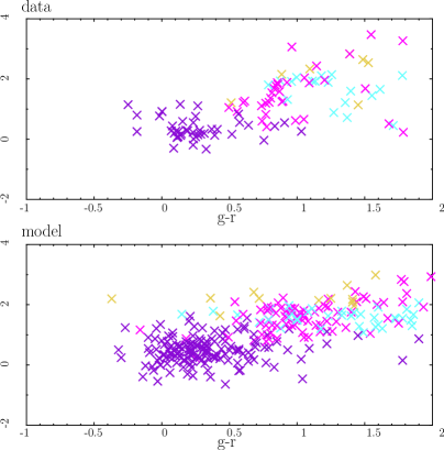
|
b) 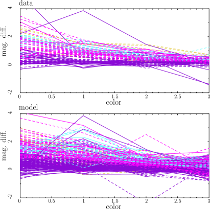
|
c) 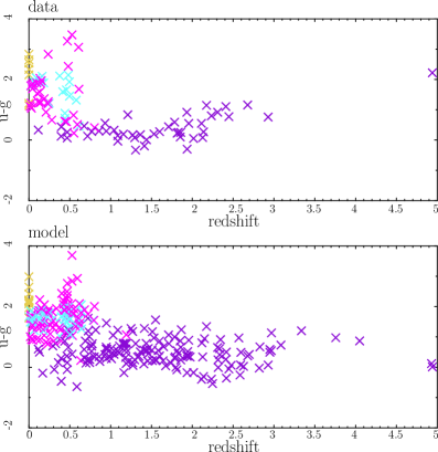
|
|
2.1 Spectroscopic Identifications
The first ChaMP public data release includes 125 spectroscopically identified sources ([Green et al.2004]). Most of them are in the medium flux category i.e. have erg sec-1 cm-2 in energy range keV keV. A small set of sources have fluxes as small as few times erg sec-1 cm-2 or as large as few times erg sec-1 cm-2 . Objects are classified in 4 categories: Broad Line Active Galaxy Nucleus (BLAGN), Narrow Emission Line Galaxy (NELG), Absorption Line Galaxy (ALG) and star. The details of criteria for associating a source to one of these categories can be found in [Green et al.2004]. For the purpose of completeness here we summarize them. BLAGN category is designated to sources with board band - FWHM km sec-1 - emission lines. If all emission lines have FWHM km sec-1, the source is classified as NELG. Objects with high and no identifying feature are classified as BL-Lac. Sources with absorption lines are classified as ALG or stars. Their spectrum is compared to synthetic templates for classification and for determination of their redshift. A classification confidence flag is given to each source: 0 not classifiable, 1 insecure, 2 secure. Here we use only sources with secure identification in the input dataset.
The set of 125 serendipitiously identified sources is too small for statistical applications. Therefore, we have added also sources from two other published set of identified sour-ces by the ChaMP, i.e. hard AGNs ([Silverman et al.2004]) and normal galaxies ([Kim et al.2006]). For this set of sourc-es as before we use the publicly available ChaMP data for x-ray, Sloan optical magnitude in 5 bands as explained above, and modeling when some of the optical magnitudes are mis-sing. After neglecting sources for which reliable data was not available and modeling couldn’t give reasonable values, we put together a total of 268 sources with identifications and all the flux/magnitude information. This set includes 151 BLAGNs, 65 NELGs. 37 ALGs and 15 stars. It is clear that in this set the number of stars is under-estimated with respect to what one can expect from a serendipidious selection of X-ray sources in high galactic latitude fields. Although the addition of ChaMP hard AGN and normal galaxies have increased the size of the learning set for the statistical identification, due to the bias of these set toward a special type of objects, the final set does not anymore presents what one can find in a set of randomly selected sources subjected only to conditions on X-ray fluxes and optical magnitudes. This is not a major problem for present work where the main purpose is the investigation of performance of classification methods. However, we will show later that the learning (input) set to algorithms or classifying agents such as humans, inevitably leaves its trace on the classification and this is inherent to the concept of learning and extension of information. This issue should be considered when the results of statistical classification are used for obtaining scientific conclusions.
3 Statistical Classification
The first step in mining X-ray selected sources is their classification. In this work we concentrate on statistical algorithms rather than automatic class/cluster finding algorithms such as neural network. The main reason for this choice is that we are searching for classes of astronomical objects which are already defined. If one of these classes happens to cluster in the available parameter space with other objects of different astronomical categories, we are not discovering a new class or property but encountering obstructions to object classification. Cluster finding methods are certainly interesting when the internal structure of the data is unknown and blind clustering helps to organize objects with similar properties to groups. This makes their studying easier.
Up to now attempts for statistical classification of X-ray sources were mostly concentrated on the relation between hardness ratios, fluxes and count rates ([Della Ceca et al.2002]; [Prestwich et al.2003]). As an example, Fig. 2-a and b show X-ray flux in ChaMP B band and hardness ratio versus hardness ratio for ChaMP identified sources described above. It is clear that there is a large overlap between parameters of different classes of sources, and therefore the addition of other information like optical/IR data is necessary for a more reliable classification ([Ziaeepour & Rosen 2003]). Recent attempts for statistical classification of ROSAT sources ([McGlynn et al.2004]; [Flesch & Hardcastle 2004]) also show a better classification efficiency when both X-ray and optical data are used. On the other hand, 2-dimensional parameter-space does not seem to be adequate. For instance, spectroscopic follow-up of Chandra and XMM-Newton sources and previous observations, show that in the medium range of X-ray fluxes and optical/IR magnitudes, most of the X-ray selected sources are BLAGN. They are mostly concentrated in a small area of and plane of optical data (Fig. 1-a), or flux and hardness ratio (Fig. 2-a), (Fig. 2-b) planes of X-ray data or even in (Fig. 2-c) when both X-ray and optical data are used. This area however contains other and rarer types of sources, and on each of these planes alone there is no significant separation of all the classes. This means that what ever the method of classification, the performance of a 2-dimensional parameter space would be low ([Ziaeepour & Rosen 2003]).
a)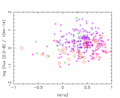
|
b)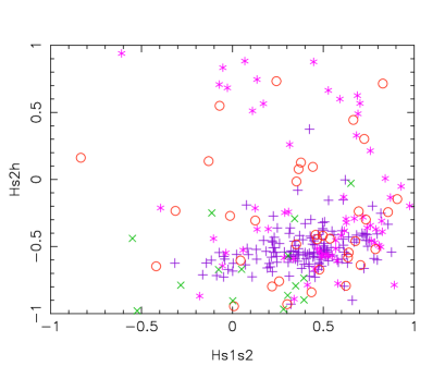
|
c)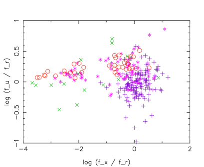
|
|
The alternative is using a multi-dimensional parameter space. In the next sections we explain a few methods of statistical classification which simultaneously explore all the available parameters. None of these methods are new, but for each application it is necessary to select the best parameters to use, the optimal number of parameters, and the performance of each method or their application in a complementary way (see below). This is the main aim of the present work.
Although using more parameters for classification leads to a greater chance for having reasonably separate clusters of objects in the parameters space, each corresponding to one category, the larger number of parameters also expands the volume to fill with the input data. Therefore, adding new parameters sometimes deteriorates the classification performance. Moreover, computational limitations, both on the amount of memory necessary for buffering the parameter space and on the CPU time for calculation, constrain the optimal parameter set, range of parameters, and their binning.
The reason for studying multiple classification models is that each of them have its own advantages and drawbacks. The choice of a method depends on the input data-set available and the application of classification results. Two main categories of applications are short-listing X-ray selected sources for further follow-up, and studying physical properties of each class. In the first case a simple but mildly precise method and a small set of input data is adequate. For the second application a much better performance and therefore a much larger input set is necessary. For instance, as we will see in more details below, classification based on the distance to a cluster of objects is not very precise. However, it needs a much smaller input (learning) set than other methods. It can be applied when only a small set of identifications is available, and one needs to have a crude classification of other sources for further investigation - for instance when only one type of source is targeted. Multiple methods can be also used as complementary to each other. As an example, in the following sections we will explain in detail a multi-dimensional probability distribution which is the best method because it uses the full parameter space and correlation between various parameters, but it needs a large input set. As a consequence, when this condition is not fulfilled, many sources can not be classified and this has an important impact on astronomically important properties such as redshift distribution. We show that in this case using less precise but also less demanding methods to classify these remaining sources leads to a better overall performance.
3.1 Performance Estimation
The usual practice for testing the performance of classification is to divide the set of known sources into two sets and use one for learning and the other for testing. At present however, our sample of identified sources is very small and dividing it to two parts certainly reduces the performance of the classification significantly and hides the real ability of methods 333For comparison it is worth to mention that the classification of the ROSAT sources in [McGlynn et al.2004] uses a selection tree method. When both X-ray and optical data are used their input set consist of 6763 RASS and 9247 WGACAT sources. When only X-ray data is used, the size of the input data is yet larger. As mentioned above we have only 268 identified sources for which all the necessary optical and X-ray data is available.. Note also that for a statically significant assessment of the performance, the test set must be also enough large. We can not use just a small subset of the identified sources for test. The test set must be enough large such that good or bad performance of the classification be statistically significant. In particular, if the input set is biased, the result of the test with a data set with very different distribution can be completely misleading. For instance, we know that in our ChaMP dataset stars are under-represented. If from this set we select a small subset of sources randomly, it can include one or two stars and the correctness of their subsequent classification is statistically insufficient to assess the quality of the classification method.
The issue of the optimal minimum size of the input set is not well understood. The suggested value in [Jain & Chandrasekaran 1982]; [Proctor 2006] is a minimum of 10 times the number of categories in the classification44410 is simply the sample length considered to be minimal statistically significant sample for most statistical applications.. In practice, the size of the input set must be much larger. In our case we want to classify X-ray selected sources to 4 types and 12 redshift ranges (see below for details). According to this prescription we need at least 480 spectroscopically identified sources. At present we have only 268 ! Nonetheless, we show that even with such a small set we can see the difference between the performance of the methods, and when they are applied to a set of unknown sources - much larger than the input set - the distribution obtained for the physical quantities such as or redshift distribution are generally what we expect.
We try various strategies to assess the performance of the methods and the effect of having to use a small set of input data. We divide the set of spectroscopically identified sources to two sets by randomly selecting each source to be member of one or the other subset. We have used an equal probability and also and . We use the larger set as input and the smaller one as test set. To see the performance in the case where a much larger input set is available, we also test algorithms by using the same set both as input and as test set. In this case for some methods such as low resolution spectrum template fitting, the classification is correct, and therefore this does not permit a performance test. But for methods based on probability distributions, this is simply similar to the case where the distribution is known (see also below for more explanation). To use the largest possible input set and largest possible test set, we have also tried another procedure 555We thank M. Page for suggesting this procedure.. In each run, we remove one of the sources from the set of spectroscopically identified sources, use the rest as input set and classify the removed source. We repeat the same procedure for all the members of the set and assess the performance by adding the result of all the iterations. This procedure needs much longer CPU time because at each iteration all the distributions must be recalculated. For this reason we apply it only to a limited number of cases. We find that this more complex test does not add much information about the performance of the method than what we conclude from simple division of available identified sources, but it helps to see that a larger input set definitively has an important impact on the classification performance.
For quantifying the performance of classification methods 3 quantities have been suggested by [Prusti et al.1992]; [Boller et al.1992]:
| Detection rate of class | (3) | ||||
| Reliability rate for class | (4) | ||||
| Contamination rate of class j in class i | |||||
Note that defined in (LABEL:contr) is not the same as false alarm rate defined by [Prusti et al.1992]; [Boller et al.1992]. They use these quantities to assess the classification IRAS sources as galaxy and non-galaxy (star). Here we have mor than just 2 categories, and the rate of contamination as defined in (LABEL:contr) is a better description of the performance of descrimination between classes. In fact the false alarm rate corresponds to the contamination rate of galaxies in non-galaxies defined in (LABEL:contr).
To assess the effect of imprecise identifications on the astronomical conclusions, we use redshift distribution of cl-asses as a benchmark. This is in fact one of the most important outcomes of the classification of a large number of X-ray selected sources. The main producers of the astronomical X-ray are accretion to black holes, star formation activities and galaxy clusters. Redshift distribution of these objects not only permits to study the evolution of star formation epochs, but also can help to better understand the issue of relation between the growing rate of super-massive black holes, AGN activities, and star formation. This has been the subject of intensive study in recent years. For stars this test is evidently irrelevant.
To quantify the closeness of distributions from spectroscopy and from statistical identification, we use a clo-seness test. For each class of objects we calculate a -like quantity as the following:
| (6) |
where is the number of sources from statistical classification in that category and in redshift bin, is the same number from spectroscopy, is the number of redshift bins with . If two distributions are exactly the same, , otherwise it can be interpreted as an average difference or goodness of fit between two distributions. We also perform a Kolmogorov-Smirnov (KS) test of the redshift distribution 666We thanks R. Della Ceca for suggesting a KS test.. In general, the conclusion of both tests about the performance is the same. The interpretation of test is however more direct and relevant for the interpretation of physical properties. The results of both tests along with quality rates defined in (3)-(LABEL:contr) are presented in Table LABEL:tab:kstest.
We want to add another remark about the relevance of these tests as a means for performance assessment specially regarding the astronomical applications of the results. KS and tests here provide a rough estimation of how reliably the redshift distribution can be recovered by using statistical algorithms. Each of them is just one number summing and smearing all the features of a distribution. In an astronomical applications however features can have special meaning and interest. In comparing two distributions, one can have smaller and KS, but for instance have a peak or trough non existent in the real distribution. They can mislead the astronomical interpretation of distributions. Moreover, large number of unclassified sources can lead to a redshift distribution quite different from the original one. Nonetheless, the method can be more precise when a source gets a classification. This is specially the case for the last method we explain in the next section. In conclusion, the performance assessment based on fit or statistical methods are incomplete and this issue must be considered in the selection of methods for astronomical applications.
4 Algorithms
In this section we describe in details classification methods we have investigated and compare their performance. They can be summarized as the followings:
-
Distance to Clusters: Each class is characterized by a vector presenting the typical place of the objects in the parameter space and a deviation matrix. Unknown objects are classified according to their distance to each class.
-
Low resolution spectrum (photometry): Fluxes are used to define a low resolution spectrum. Unknown sou-rces are classified both for their type and their redshift by fitting their spectrum to templates. This method is essentially the traditional photometric redshift determination to which we have also added the classification of sources.
-
Parameters as independent measures: Each measured quantity is considered as an independent identifier of a class. For each class its distribution is determined, and Maximum Likelihood (ML) is used to estimate the likelihood for an object to belong to a class and a redshift.
-
Multi-dimensional probability: The whole parameter space is used for the classification by binning parameters and calculating multi-dimensional probability distribution for each class. Unknown sources are classified according to the conditional probability to belong to one of the classes.
The results of all classification methods and their tests are summarized in Table LABEL:tab:kstest.
4.1 Distance to Clusters
This method is a variant of the clustering algorithm ([Everitt 1993]) in which an object is classified with respect to its distance to clusters of known sources. Clusters are defined by a vector presenting the center of the cluster and a deviation (covariance) matrix:
where and are respectively center and deviation matrix of class, and are respectively the dimension of the parameter space and the number of input sources of type . To classify an unknown source, its deviation from the center of each cluster is calculated, and it is associated to the closest cluster/class if its distance from the center of the cluster is smaller than the deviation of the class, otherwise it is marked as unclassifiable. The performance of this method is moderate, see Table LABEL:tab:kstest. Parameter space that has been used for this method and others is also defined in this table.
Another variation of cluster method is calculating distances to clusters projected to two subspaces of parameters. For the object:
| (8) |
where is the dimension of the first subspace and is the dimension of the second subspace. Distribution of known sources in the 2-dimensional space is used for classification.
A natural choice for subspaces in our case is optical and X-ray parameters. After binning parameters, in each subspace we determine the Euclidean distance (4.1) with respect to the origin - the bin with smallest index (i.e. zero) for all the parameters. Normalization can be performed by choosing the same number of bins for all the parameters, otherwise the effect of parameters with more bins would be more than others. This also can be considered as a weight given to parameters which are more important in distinguishing one class from others.
The result is a distribution in a 2-dimensional space wh-ose coordinates correspond to distances in optical and X-ray subspaces as defined above. This space is normalized with respect to bin with the maximum number of entries and binned. As the parameter space in this procedure is truncated, it is more meaningful to normalize it with respect to maximum than with respect to total number of entries. This normalization somehow amplifies features in the distribution and helps classification, whereas normalization to total number of entries makes the distribution flatter and featureless. This definition is possible because distributions are considered as being the conditional distribution in the parameter space. The final distribution is normalized as usual to make the total conditional probability equal 1. Distances and thereby the distribution of sources in each subspace depends on the parameters. Fig. 3 shows an example of distribution of sources.
a)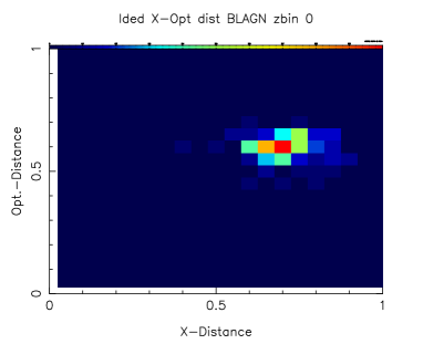
|
b)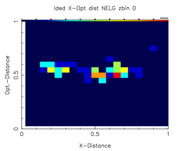
|
c)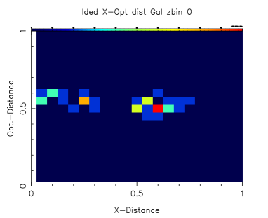
|
d)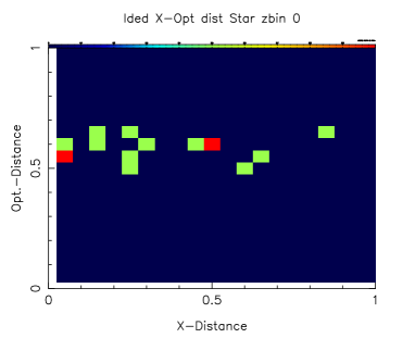
|
e)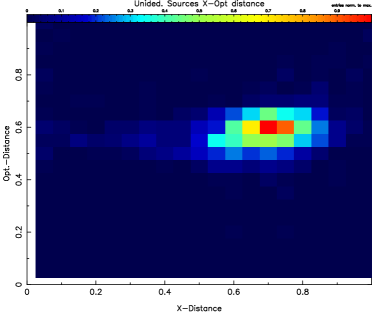
|
|
The conditional probability for an unknown source to belong to a class is directly obtained from these distributions. Due to the existence of many empty bins in the parameter space, we smear bins by considering not only the probability of the bin to which the unknown source belongs, but also its neighbors, and determine an average probability. Then, we compare this probability with the same quantity for other classes. The source is associated to the category with the highest probability. We also request a minimum probability of where is the total surface of the 2-dimensional distribution777This corresponds to the probability for each bin in a uniform distribution. If objects were distributed uniformly in the parameter space, no classification could be done.. If this condition is not satisfied, the source is considered to be unclassifiable.
The performance of this algorithm is much better than the first one. The result is summarized in Table LABEL:tab:kstest. Although this method is not able to discriminate redshifts, it is fairly good in classification specially when the input set is small. Fig. 4 compares the X-ray - for 125 classified sources using an input set of 143 sources. The largest difference is for stars which are under-represented - only 8 stars in the input sample.
a) 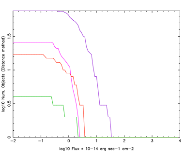
|
b) 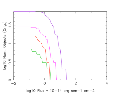
|
4.2 Low Resolution Spectra
This method has been inspired from the photometric redshift calculation.
One way of determining redshift from photometric data is to compare the
photometric measurements of the source, considered as a low resolution
spectrum, to templates ([Miralles & Pelló 1998]). Various methods for cla-ssification
have been used including: analytical parameterization ([Connolly et al.1995]),
-fitting ([Miralles & Pelló 1998]), maximum likelihood ([Wolf et al.2001],
[Wolf et al.2004]), and
neural network ([Collister & Lahav 2004]). In this section we discuss -fitting
and in the next section the maximum likelihood algorithm.
For fitting we have tried two procedures. In the first procedure, we use optical/IR and X-ray fluxes of the spectroscopically identified sources to determine an average low resolution spectrum, and a dispersion (standard deviation) around the average curve for each class and redshift bin defined in Table 2. These spectra are used as templates. We use the same redshift binning for all the methods. The choice of the bins is simply conducted by having a significant number of input sources in each bin. The number of bins is also limited by the size of memory necessary for buffering the corresponding probability distributions (see Sec.4.4).
The spectrum of each unclassified source is compared to these templates according to difference defined as:
| (9) |
where includes both the dispersion around the average and measurement errors; is the average value of parameter in the input data set. We note that measurement errors are much smaller than the intrinsic dispersion of the population and don’t significantly contribute in . The unclassified source is associated to the class and redshift bin with smallest . If all where is the number of freedom degrees, the source is considered to be unclassifiable. For , this is roughly equivalent to probability that the source belongs to one of the categories but be rejected.
In the second procedure we simply fit the spectrum of the unclassified sources to spectrum of all the members of the available input data set by using equation (9). For the uncertainty we have tried measurement errors, dispersion as explained for the first procedure, and simple normalization to the template. We find that measurement errors are too small as deviation estimation, becomes too large, and the result of the classification becomes biased to the dominant population of sources i.e. to BLAGN (which has the smallest dispersion). Two other dispersion estimations are better and give more or less the same results. In both cases depending on the parameter space - normalisation of fluxes by optical or X-ray flux - either stars are over-estimated and ALG underestimated or vis-versa. The redshift discrimination quality of these dispersion estimation methods are also very similar, although the details of the redshift distribution curve can be different. In summary, we can not find any criteria preferring one of the dispersion estimation to the other.
The performance of the two spectrum fitting procedures explained here is not very different, but fitting to all sources separately is somehow better in classifying BLAGNs - the dominant population of the X-ray selected sources888The reason for a better performance of fitting individual sources can be the small dispersion of BLAGN spectra. There is more chance to find an identified source with very similar spectrum for this class of objects.. Therefore, here we only report the results of this procedure.
| Band | Redshift | Band | Redshift |
|---|---|---|---|
| B1 | z 10-2 | B7 | 1.25 z 1.5 |
| B2 | 10 z 0.25 | B8 | 1.5 z 1.75 |
| B3 | 0.25 z 0.5 | B9 | 1.75 z 2 |
| B4 | 0.5 z 0.75 | B10 | 2 z 2.5 |
| B5 | 0.75 z 1 | B11 | 2.5 z 3.5 |
| B6 | 1 z 1.25 | B12 | z 3.5 |
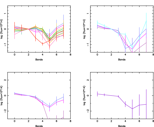 |
The performance of this method is better than distance to clusters. Under conditions we have imposed on the fit, the number of unclassified sources emerging from this method is only a few percents. The fraction of good classifications somehow depends on the quantity used to represent the spe-ctrum. We have tried a number of quantities including: logarithm of fluxes; relative fluxes to the Chandra broad B-band flux , where presents all other available X-ray and optical/IR bands; relative fluxes to one of the optical fluxes ; flux ratio of successive bins (color); and photon number flux (calculated from energy flux) where is the mean energy of the band. We have found that the best combinations are relative fluxes to optical band or to X-ray B band. For testing this algorithm we can not use the same data both for input and for test. Therefore, all the results in this section are based on completely independent input and test sets.
With this algorithm BLAGNs are correctly classified in of cases, but are under-estimated. There is an over-estimation of NELG where in most cases the spectroscopic identification is BLAGN or ALG. Due to under-representa-tion of stars in our data set, their classification is in general poor. Depending on the parameter space, either they are not correctly classified or there are many contaminations from other categories. Nonetheless, our experience with the XMM-Newton data shows ([Ziaeepour & Rosen 2005]) that when significant number of stars are present in the input data set, this method is well capable of classifying them.
It is worth to remind that all the classification methods explained in this work are based on conditional (Bayesian) probability. Therefore, the ideal case is to have the same number of sources for each class and redshift in the input set. In practice however, it is very difficult to collect such a set of identified sources as their occurrence in the serendipitous data is quite different.
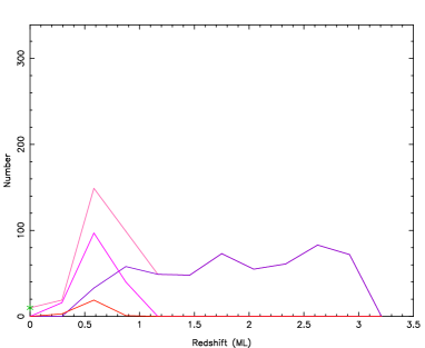
The precision of the recovered redshift in this method is more modest . Nonetheless, of incorrect redshifts have only bin of difference from the spectroscopic redshift which, for , means . Fig. 6 compares the redshift distributions of classified sources by this method with the spectroscopic ones. To see if reducing the number of redshift bins improves the performance of redshift determination, we have also tested this algorithm with only 6 redshift bins with . We find that the performance is practically the same (see Table LABEL:tab:kstest). The reason can be the fact that by averaging/binning spectra in too large intervals we smear critical redshift dependent features.
Because this method is used by many optical/IR surveys ([Miralles & Pelló 1998]) for photometric redshift determination, it is worth to mention that the reason for their performance is the large input sets of thousands or even tens of thousand of spectroscopically classified spectra. At present such an input set is not available for X-ray surveys, and therefore they should use more ingenious algorithms for classification.
a)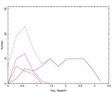
|
b)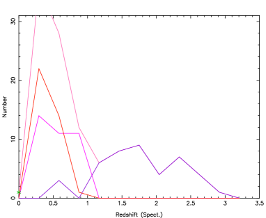
|
c)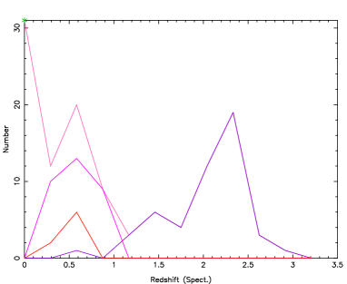
|
|
4.3 Parameters as Independent Measurements
This popular method for hypothesis/model testing uses each measurement as an independent observation of the hypothesis/model under scrutiny. For classification of astronomical sources, the measured value of various physical parameters can play the role of independent observations 999The way we use maximum likelihood here is somewhat different to its usual application. For parameter estimation, usually one quantity is measured for fixed values of another parameter. The distribution for all the measurements is assumed to be the same. A good example is the application of ML to Cosmic Microwave Background (CMB) anisotropy for estimation of cosmological parameters. In this case the observed quantity is the anisotropy at different angular scales. In classification problem we have one measurement but multiple quantities with different distributions. Therefore the mathematical meaning of the likelihood here is not exactly the same as usual. This is not a concern because our aim is classification of objects and not their statistics. Therefore, any means that can discriminate them is appreciated.. We should not however forget that usually these parameters - in our case X-ray and optical fluxes - are not independent. Nonetheless, their relations are subtle and linear methods such as principal component analysis are not appropriate for finding independent combinations. Moreover, different classes can have different sets of independent parameters. This makes the definition of one set of parameter for all classes impossible. Therefore, we simply use this method without any attempt to reduce the number of parameters or find an independent set. We neglect their correlations and use the maximum likelihood method to find the probability distribution for each parameter, each class and each redshift. An example of these 1-dimensional distributions is shown in Fig. 7. The main conclusion we make from this figure is that NELGs, ALGs and stars have very similar distributions. BLAGNs are somehow different from other categories, but they cover the same region of the parameter space, and there is no special feature capable of singling out just one category of sources. This conclusion is also consistent with 2-dimensional distributions in Figs. 2.
a)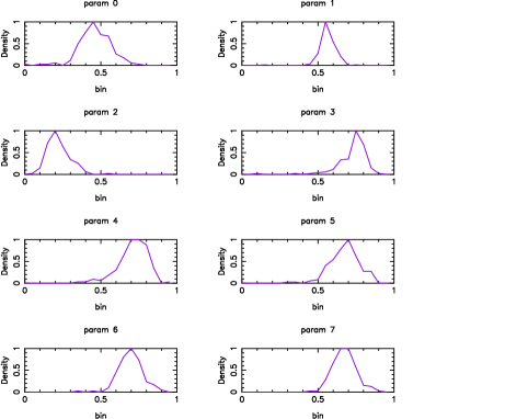
|
b)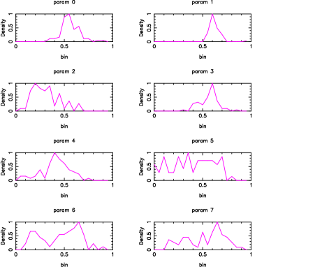
|
c)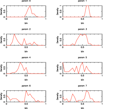
|
d)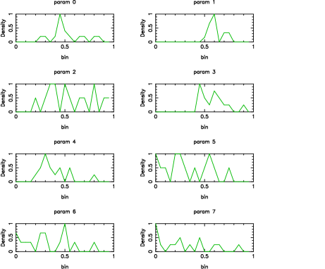
|
For each unclassified source we calculated its likelihood to belong to a class and redshift bin as the following:
| (10) |
where is the distribution of parameter calculated using spectroscopically identified sources and is the measured value of parameter for the unclassified source. Similar to the distance method we request a minimum value for likelihood . Sources with likelihoods less than this lower limit for all categories and redshift bins are considered as unclassifiable.
Mathematically, ML method and -fitting explained in the Sec.4.2 are both based on 1-dimensional distribution of parameters. Their difference when they are applied to classification problem is in the way they treat the input data. In -fitting if we fit the spectrum of an unknown source to a template for each class, it is equivalent to considering a 1-dimensional Gaussian distribution for each parameter around the corresponding value for the template. From Fig. 7 it is clear that parameters used here don’t have Gaussian distributions. If we fit the spectrum of an unclassified source to all the available sources to find the most similar source, one of them eventually will have the smallest , but we don’t explore the statistical properties of the available input set i.e. how frequently one type of spectrum occurs. Moreover there is no way to fill the gap between different templates by for instance interpolation. In contrast, ML method is not based on any predefined distribution for parameters and gets the information directly from the learning sample. As a result the performance of this method is much better than -fitting.
We use the same parameter space as that adopted for the low resolution spectrum method, i.e. either or with indicating other X-ray or optical/IR bands. For binning each measurement, the range of possible values must be defined. We fix the range for each parameter such that it is covered by the largest input data set available. Evidently, for unclassified sources we can not guarantee that they will fall in the same range. Therefore apriori we should consider a larger range. But the input probability distribution in these regions would be zero and will not help the identification. In practice when a measurement is out of range, we associate it to the closest bin i.e. to the first or the last bin. In any case the definition of the volume of the parameter space affects classification and we have not found an optimum prescription. This issue is relevant for both 1-dimensional and multi-dimensional distributions.
The performance of the maximum likelihood method is very good, for both a low number of unclassified sources and good estimation of redshift distribution, see Table LABEL:tab:kstest and Fig. 8. Like previous methods, the performance for classification of stars is poor, but we attribute this to the under-representation of the stars in our input set rather than the fault of the algorithm.
Because this method is based on 1-dimensional distributions, we can use the same data set for input and for test. This is equivalent to assuming distributions to be exact, i.e. when the size of the input set goes to infinity. Tests with independent sets also show roughly the same level of performance.
a)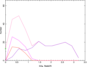 b) b)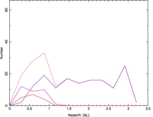 c) c)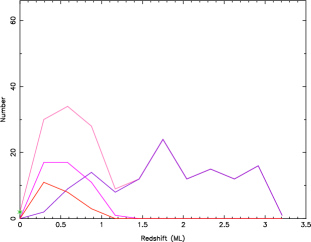
|
Despite the efficiency of this method for moderate size input set, it is not sure that it keeps the same performance for large number of sources when 1-dimensional distributions approaches uniformity. The evidence for such concern comes from the classification of 1357 unknown ChaMP so-urces in Fig 9 by this method. Redshift distribution of 718 sources that got classification looks very similar to the input set. If our input distribution was very close to the cosmological distribution, we evidently expected such behaviour. But we know that our input data set of 268 sources is very far from being the unbiased cosmological distribution, and therefore the similarity of the redshift distribution to the input is an evidence of fast saturation of the algorithm. The problem of having close to uniform 1-dimensional distributions can be solved by making finer redshift bins. Apriori the bias toward the input distribution is not a problem if the input set is unbiased. Otherwise, we should expect a relative deterioration of classification for large input data sets. This seems somehow counterintuitive because classification of each source is independent of others. The deterioration is however due to the accumulation of errors, otherwise the probability of wrong classification per source is always the same.
4.4 Multi-dimensional Probability
The space of all independently measured quantities contains all the available information about sources and includes all the correlations between parameters which can be used for discriminating between various classes ([Prosper 2000]). As we mentioned before, although based on physical argument-s there must be a relation between various fluxes, their correlations are complicated and nonlinear. The visual demonstration of the complexity of distribution in a multidimensional parameter space is difficult. Nonetheless, the diversity of low resolution spectra (see Fig. 5) and 2-dimensional projections such as Fig. 3 and Fig. 2 are the evidence for this claim. A linear relation between a subset of parameters in a dimensional parameter space makes sources cluster in a dimensional subspace. If data has such a structure, it must show up at least in some of the 2-dimensional projections, and the distribution of sources should have an approximately axial symmetry in the direction of the projected principal component. We have tried various combination of 2-dimensional projections and find no symmetries permitting a reduction of the parameter space. This means that application of a dimensional reduction algorithm like principal component does not help to reduce the volume without losing important information. The only possible optimization of the volume of the parameter space is therefore based on the choice of the range of parameters, as mentioned in the previous section.
For exploring the multi-dimensional distribution of sou-rces in the parameter space, we are obliged to restrict its dimension and/or the number of bins for each parameter101010In the current versions of the GNU compiler, the memory allocation is limited to 2 GB corresponding to 4-byte addressing, and the total allocated buffer by the code can not exceed this value.. We have found that the performance is much more sensitive to X-ray than optical flux binning. The reason seems to be a higher variation of X-ray fluxes than optical ones (see Fig. 5). The reason can be simply the wider band-width of X-ray - about 1.5 orders of magnitude - than optical filters band-width which, from to , is less than 0.5 orders of magnitude. When 4 or 5 optical fluxes are used, we consider 6 bins for each optical flux ratio and 8 bins for each X-ray one. For less than 4 optical fluxes, 8 bins are used for optical and 10 for X-ray fluxes.
a)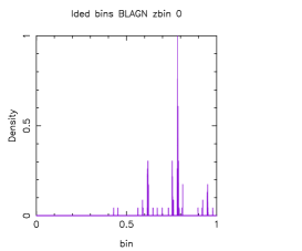
|
b)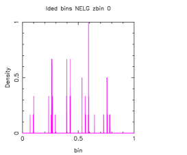
|
c)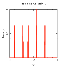
|
d)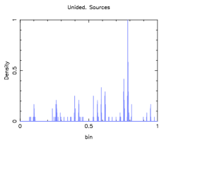
|
After distributing spectroscopically identified sources in each class and redshift bin, distributions are normalized in the same way explained in Sec.4.1 and considered to be the multi-dimensional probability density for each class and redshift. To classify an unclassified source, its place in the parameter space is determined in the same way and its probability to belong to a class and a redshift bin is determined from multi-dimensional distributions. Due to the small nu-mber of sources in the input, we use a smeared probability i.e. for each class we don’t use only the probability of the bin to which the unclassified source belongs but also the closest neighbour bins and determine an average probability (without weighting). Averaging can be removed if the input set is sufficiently large. We also consider a minimum probability inversely proportional to the total volume of the parameter space. If for all classes and redshifts the probability is smaller than this limit, we consider the source as unclassifiable.
Despite the large parameter volume of this method and relatively small number of input sources available, it has the best performance both in classification of sources and in determination of redshifts. When the same data set is used for input and test - equivalent of having either the exact distribution or when the size of input set is very large - the identification performance is close to and redshift classification (see Table LABEL:tab:kstest for details). When independent input and test sets are used, many sources are left unclassified and the performance of redshift classification is more modest. This has a serious impact on the redshift distribution curve, see Fig. 11. One can therefore conclude that for this method a much larger input data set is necessary. Evidently, this is not a surprise as the volume of the parameter space is much larger than when 1-dimensional distributions are used.
a)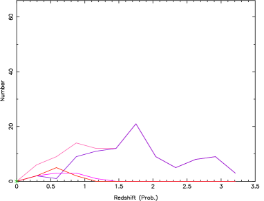
|
b)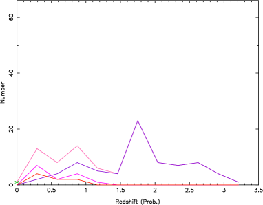
|
The problem of unclassified sources can be partially sol-ved if we use multi-dimensional probability along with ma-ximum likelihood and low resolution spectrum. Fig. 12 sho-ws the redshift distribution of statistically classified sources by applying first multi-dimensional probability and when a source can not be identified by this method applying, by order of priority, ML or low resolution spectrum fit. In this way, not only many of unclassified sources get classified, but also the result of the KS and tests show that the redshift distribution becomes much closer to the one from spectroscopy. Fig. 12 shows the distribution of the same sources in the X-ray-optical flux plane and demonstrates how the complementary use of multiple methods can improve classification. Nonetheless, our tests with various divisions of the available data set and choices of parameters show that when multiple methods with various degree of precision are used in a complementary manner, the contribution of less precise algorithms must be kept small otherwise they reduce the overall performance. They should be applied only when more precise methods can not classify a source, and if possible, other constraints such as higher minimum probability should be applied.
We should also mention that the large amount of memory necessary for buffering each distribution is an important limit for application of this method to finer redshift division even when in each redshift bin enough input data is available. The solution can be a multi-step classification: First sources are classified in a category and relatively large redshift band. Then, multi-dimensional probability or another method such as maximum likelihood can be used to classify them in finer redshift bands.
a)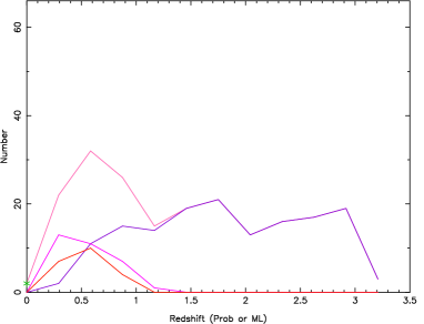 b) b)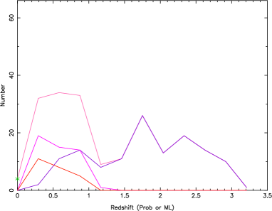
|
Finally, we discuss the role of various optical filters in the statistical classification of X-ray selected sources. This issue is important for optimizing the time and effort needed for optical follow-up and imaging. Fig. 13 shows the redshift distribution of sources when only , and optical fluxes are used. We find that the impact on the classification is not very significant, but the redshift distribution is somehow affected.
a)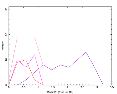
|
b)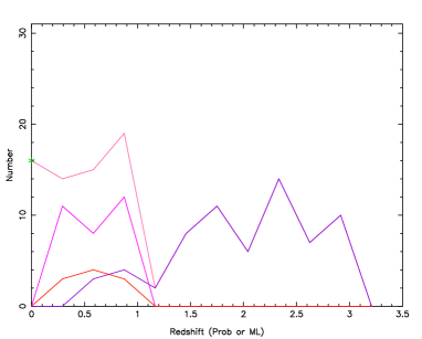
|
4.5 General Notes about Statistical Classification
A general characteristic of all the methods we have discussed in this work is that although they are based on learning - no predefined rule or relation between parameters of a class is implemented in the algorithms - they don’t extrapolate the input knowledge. If a source has parameters in a part of the parameter space uncovered by the input data, there is no way to guess its class. Averaging the probability in neighbour bins can partially compensate for the lack of information, but it is not useful when the input distributions are very disconnected because of their limited size. The same type of problem exists for nearest neighbour algorithm in which although isolated entries can be always related to a nearest class, the reality of the association is very doubtful.
One way of improving the knowledge about the distribution of classes in the parameter space is to add statistically classified sources to the initial input data and re-access the probability distribution. When the distribution is not too disconnected this procedure helps to extend the knowledge to part of the parameter space uncovered by the initial data and to improve the probability estimation. The weak point of this procedure is that if initially the classification performance is uncertain, by adding incorrectly classified sources to the learning set, errors accumulate and deteriorate the classification performance.
To test the possibility of knowledge extension and the performance of statistical classifications of unknown Cha-MP sources shown in Fig. 9, we use these sources as input data to the classification algorithm and statistically classify the spectroscopically identified sources. We make two separate data sets for the parameter spaces described in Fig. 11. We note that according to this plot and Table LABEL:tab:kstest when the ratio of fluxes to optical flux are used, there is a clear bias toward stars and under-representation of ALG/gal in the classification. Consequently, we expect that the corresponding statistically classified sources as input to the algorithms must be a poorer classifier than when the parameter space is define by ratio of flux to the X-ray B band. This is exactly what we find when we use these sets to reclassify spectroscopically identified sources, see Fig. 14. For less biased parameter space of flux ratios to X-ray B band as input set, the number of detected stars is very close to the exact value (16 in place of 15), in contrast, to the cases when all or part of the ChaMP identified sources have been used as input. The parameter space defined from ratio of flux to optical band over estimates stars.
As we mentioned before, stars are under-represented in our set of spectroscopically identified sources. In the statistically classified set their fraction is more significant (see Table LABEL:tab:kstest for details). This leads to a better classification of stars when this set is used for learning. This is clear evidence of knowledge extension. Moreover, this investigation hints to a methodology for testing the quality of classification of unknown objects by inverting the place of learning and output data sets.
a)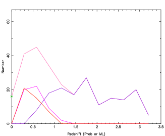
|
b)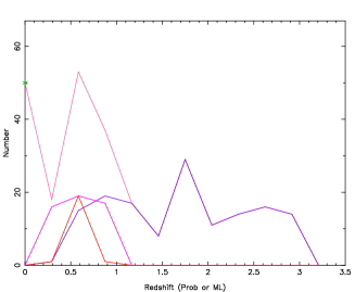
|
c)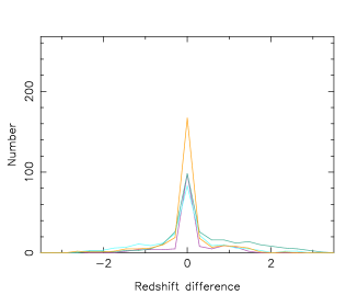
|
|
Another strategy for knowledge enhancement that can be also applied to disconnected distributions is automatic rule detection. This concept is in some ways similar to automatic cluster detection. However, attempts here should be concentrated on finding extendable features like symmetries because clustering is already included in the probability distribution. For instance, searching the principal component for a subclass, a class or multiple classes can help to find a symmetry axis for that group of sources. Fig. 15 shows that BLAGN have a roughly oblique elliptical distribution in X-ray-optical flux plane. Assuming that this behaviour is extendable to a larger sample, one can use the closeness to symmetry (principal component) axis to classify sources. We leave this investigation to a future work when more spectroscopically identified sources are available. Note also that this figure confirms that we can not use principal component analysis to reduce the number of parameters or find uncorrelated quantities for all the X-ray sources because different classes have different set of approximately independent parameters.
a)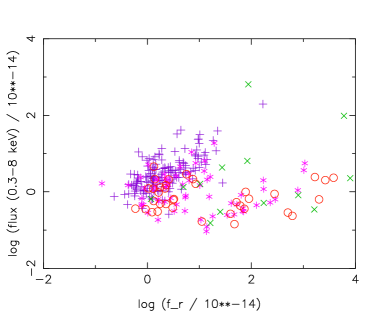
|
b)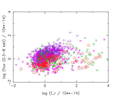
|
5 Effect of Statistical Classification on Physical Conclusions
Irrespective of the method used for statistical classification, the input set leaves its fingerprint on the physical conclusions. Therefore, only if the input data is sufficiently - with but a few percent of fluctuations - representative of the wh-ole population, one can be confident on the reliability of the deduced conclusions about the physical behaviours from statistical classification. By giving some examples in this section, we show that the available data set is yet too small and a much larger input set is needed. At the same time, these examples clarify how one should investigate artifacts left in the output of the statistical classification from the input data or classification methods.
We have already seen in Fig. 14 the effect of under-representation or over representation of a category of objects on the classification. Fig. 16 shows the distribution of corresponding statistically classified sources in - plane. Suppose that from these plots we want to judge about X-ray to optical luminosity of different category of sources. According to the biased population of Fig. 16-b, significant number of stars have a very hard spectrum i.e. . But less biased classification of Fig. 16-a and spectroscopically classified sources Fig. 16-c don’t show such a population. Similar effects are also visible at low X-ray luminosity, low X-ray to optical flux tail where in Fig. 16-b this area is dominated by stars but Figs. 16-a and 16-c show a significant contribution from NELG and ALG/gal. This has important implications for absorption column density in these types of extra-galactic objects.
a)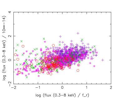
|
b)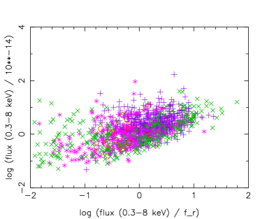
|
c)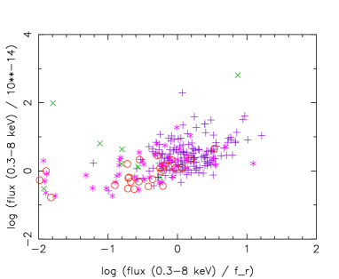
|
|
These are examples of misleading conclusions due to incorrect classification. Thus before any scientific conclusion be taken from statistical classifications, we must first assess their uncertainty and its effect. One way to take this into account could be to add an uncertainty to the distributions coming from a statistical classification. This is not however a simple task. The test of a classification algorithm is based on a small sample in which a classification bias can be difficult to detect. When such a method is applied to unknown objects, it is very difficult to know whether an observed behaviour of data is intrinsic or due to wrong classification. Moreover, quantifying the uncertainty of distributions is not simple either. We must also add the uncertainty about how representative is the set of spectroscopic identifications to classification uncertainty. There are a few more issues also to consider: to what extent is the selection of a source for spectroscopic follow-up a random process ? How much do observational conditions, source location on the sky, visibility to a special telescope, etc. bias the selection of sources for follow-up ? Or in general, does the set of followed-up fields present a random sampling of the whole sky ? One way to answer these questions is to divide the sample, plot separate parts and try to find any systematic difference. This is possible only if the size of the sample is enough large such that it can be dived to statistically significant subsets.
Before concluding this section we want to add few remarks about the general purpose of statistical identification, in X-ray or other domains of astronomy. As we mentioned in this and previous sections, whatever the classification me-thod, the input data set leaves its imprint on the statistical identified sources. This is quite natural because it is the base of information. Then, the question arises: what more we can learn about astronomical issues than what is in the input (learning) set ? Probably the most important and unbiased ones are issues related to quantities which are not used in the process of classification. For instance, large scale spatial correlation of different type of objects. More applications can be found with combination of observables used in the classification - here fluxes - and what is not used in classification such as spacial distribution. Note also that redshift is not an independent quantity because it is estimated from the knowledge coming from the input set.
6 Conclusion
We have studied a number of statistical methods for automatically classifying X-ray selected sources with optical follow-up. We have found that a multi-dimensional probability technique that includes maximum information ab-out the sources is the best method although it needs a large input set. When enough input data is available, with this method BLAGN and stars which are dominant sources in the population of the medium and bright X-ray sources, are correctly identified in of cases. Redshift distribution can be also recovered with reasonable accuracy. In absence of a large input set, a complementary use of various methods can improve classification. An interesting point about all the algorithms is that they are quite sensitive to the parameter space and their performance can be significantly improved with a proper choice of parameters. We also studied the effect of the input data set and parameter space on the characteristics and relation between physical quantities deduced from the statistically classified sources, and showed that astronomical conclusions are sensitive both to the input set and to the classification method. Nonetheless, because for each class and redshift bin we determine a conditional probability, if there is enough information about distribution of parameters within a category/redshift, classification can have good performance even when the relative contribution of categories in the input sample is different from cosmological one.
The general conclusion of this work is that statistical classification of X-ray selected sources by some of the me-thods described in this work can be sufficiently accurate to be used for astronomical ends. A larger set of spectroscopically identified sources is however necessary to improve the statistical significance of classifications as well as features detected in the statistically classified data. When a significant fraction of ChaMP fields are spectroscopically followed up, it would be possible to apply these methods to a large fraction of the sky and investigate various astronomical issues from correlation of Large Scale Structures in X-ray and optical, star formation history and evolution of super-massive black holes, etc.
Acknowledgment We would like to thank: The ChaMP collaboration for putting their valuable data in public access and Kinwah Wu for suggesting the use of ChaMP data for this work.
References
- [Barcons et al.2002] Barcons, X., et al.: 2002, A.&A. 382, 522 (astro-ph/0110269).
- [Barcons et al.2003] Barcons, X., et al.: 2003, AN 324, 44 (astro-ph/0211533).
- [Barger et al.2001a] Barger, A.J., et al.: 2001, Astron.J. 121, 662.
- [Barger et al.2001b] Barger, A.J., et al.: 2001, Astron.J. 122, 2177 (astro-ph/0106219).
- [Bauer et al.2004] Bauer, F.E., et al.: 2004, Astron.J. 128, 2048 (astro-ph/0408001).
- [Boller et al.1992] Boller, Th., Meurs, E.J.A., Adorf, H.M. : 1992, A.&A. 259, 101.
- [Brandt et al.2002] Brandt, W.N., et al.: 2002, astro-ph/0212082.
- [Brandt & Kaspi 2003] Brandt, W.N., Kaspi, S.: 2003, AIP Conf.Proc. 645, 119 (astro-ph/0208248).
- [Brett et al.2004] Brett, D.R., West, R.G., Wheatley, P.J.: 2004, MNRAS 353, 369 (astro-ph/0408118).
- [Carpenter & Grossberg 1991] Carpenter, G.A., Grossberg, S.: 1991, “Pattern Recognition by Self-Organizing Neural Networks”, MIT Press, Cambridge, MA.
- [Cohen 2003] Cohen, J.: 2003, ApJ. 598, 288.
- [Collister & Lahav 2004] Collister, A.A., Lahav, O.: 2004, Publ.Astron.Soc.Pac. 16, 345 (astro-ph/0311058).
- [Comastri et al.(2002)] Comastri, A., et al.: 2002, astro-ph/0203019.
- [Comastri et al.2003] Comastri, A., et al.: 2003, AN 324, 28 (astro-ph/0211306).
- [Connolly et al.1995] Connolly, A.J., et al.: 1995, Astron.J. 110, 2655 (astro-ph/9508100).
- [Cowie et al.2003] Cowie, L., et al.: 2003, ApJ. 584, L57.
- [Della Ceca et al.2002] Della Ceca, R., et al.: 2002, astro-ph/0202150.
- [Della Ceca et al.2004] Della Ceca, R., et al.: 2004, A.&A. 428, 383 (astro-ph/0407481).
- [De Luca & Molendi 2004] De Luca, A., Molendi, S.: 2004, A.&A. 419, 837 (astro-ph/0402233).
- [Everitt 1993] Everitt, B.S.: 1993, “Cluster analysis” Arnold, E., London.
- [Flesch & Hardcastle 2004] Flesch, E., Hardcastle, M.J.: 2004, A.&A. 427, 387 (astro-ph/0407310).
- [Franceschini et al.2005] Franceschini, A., et al.: 2005, Astron.J. 129, 2074 (astro-ph/0412476)
- [Gandhi & Fabian 2003] Gandhi, P., Fabian, A.C.: 2003, MNRAS 339, 1095 (astro-ph/0211129).
- [Georgakakis et al.2004] Georgakakis, A., et al.: 2004, MNRAS 349, 135 (astro-ph/0311609).
- [Ghosh 2002] Ghosh P.: 2002, astro-ph/0203321.
- [Giacconi et al.2001] Giacconi, R., et al.: 2001, ApJ. 551, 624.
- [Granato et al.2002] Granato, G.L., et al.: 2002, astro-ph/0208330.
- [Green et al.2004] Green, P.J., et al.: 2004, ApJ. 150, 43.
- [Jain & Chandrasekaran 1982] Jain, A.K., Chandrasekaran, B.: 1982, “Hand book of Statistics”, Vol. 2, eds. Krishnaiah, P.R., Kanal, L.N..
- [Jain & Dubes 1988] Jain, A.K. and Dubes, R.C.: 1988, “Algorithms for Clustring Data”, Prentice Hall, Englewood Cliffs, New Jersey.
- [Kim & Elvis 1999] Kim, D.W., Elvis, M.: 1999, ApJ. 516, 9.
- [Kim et al.2004] Kim, D.W., et al.: 2004, ApJS. 150, 19,: 2004, ApJ. 600, 59.
- [Kim et al.2006] Kim, D.W., et al.: 2006, ApJ. 644, 829 (astro-ph/0512338).
- [King 2004] King, A.R.: 2004, MNRAS 347, L18.
- [Kohonen 1995] Kohonen, T.: 1995 “Self-Organizing Maps”, Springer, Berlin.
- [Komossa & Hasinger 2002] Komossa, S., Hasinger, G.: 2002, astro-ph/0207321.
- [Krzanowski 1998] Krzanowski, W.J.: 1998, J.Classification 15, 81.
- [Maiolino et al.2000] Maiolino, R., et al.: 2000, A.&A. 355, L47 (astro-ph/0002447).
- [Matt et al.2003] Matt, G., Guainazzi, M., Maiolino, R.: 2003, MNRAS 342, 422 (astro-ph/0302328).
- [McGlynn et al.2004] McGlynn, T.A., et al.: 2004, ApJ. 616, 1284.
- [Michie et al.1994] Michie, D., Spiegelhalter, D.J., Taylor, C.C. (eds): 1994, “Machine Learning, Neural and Statistical Classification”, Ellis Horwood, online version: “http://www.amsta.leeds.ac.uk/ charles/statlog/”.
- [Miralles & Pelló 1998] Miralles, J.M., Pelló, R.: 1998, astro-ph/9801062.
- [Miyaji et al.2000] Miyaji, T., Hasinger, G., Schmidt, M.: 2000, A.&A. 353, 25.
- [Norman et al.2004] Norman, C., et al.: 2004, ApJ. 607, 721.
- [Page et al.2000] Page, M.J., Mittaz, J.P.D., Carrera, F.J. : 2000, MNRAS 318, 1073.
- [Piconcelli et al.2003] Piconcelli, E., et al.: 2003, A.&A. 412, 689 (astro-ph/0309606).
- [Prestwich et al.2003] Prestwich, A.H., et al.: 2003, ApJ. 595, 719 (astro-ph/0206127).
- [Proctor 2006] Proctor, D.D.: 2006, ApJS. 165, 95 (astro-ph/0605104).
- [Prosper 2000] Prosper, H.B.: 2000, hep-ph/0006356.
- [Prusti et al.1992] Prusti, T., Adorf, H.M., Meurs, E.J.A.: 1992, A.&A. 261, 685.
- [Risaliti et al.2000] Risaliti, G., et al.: 2000, A.&A. 357, 13 (astro-ph/0002460).
- [Silva et al.2004] Silva, L., Maiolino, R., and Granato,G.L.: 2004, MNRAS 355, 973 (astro-ph/0403381).
- [Silverman et al.2004] Silverman, J., et al.: 2004, ApJ. 618, 123(astro-ph/0409337).
- [Silverman et al.2005] Silverman, J., et al.: 2005, astro-ph/0511552.
- [Sipior et al.2003] Sipior, M.S., Eracleous, M., and Sigurdsson, S.: 2003, astro-ph/0308077.
- [Soltan et al.2005] Soltan, A.M., Freyberg, M.J., Hasinger, G.: 2005, A.&A. 436, 67 (astro-ph/0501275).
- [Steffen et al.2004] Steffen, A.T., et al.: 2004, Astron.J. 128, 1483 (astro-ph/409088).
- [Tozzi et al.2001] Tozzi, P., et al.: 2001, ApJ. 562, 42 (astro-ph/0103014).
- [Ueda et al.2003] Ueda, Y., et al.: 2003, ApJ. 598, 886.
- [van Speybroeck 1997] van Speybroeck, L., et al.: Proc. SPIE, 3113 (1997) 89.
- [Wilkes 2002] Wilkes, B.J.: 2002, ApJ. 564, L65.
- [Wolf et al.2001] Wolf, C., Meisenheimer, K., R ser, H.-J.: 2001, A.&A. 365, 660 (astro-ph/0010092).
- [Wolf et al.2004] Wolf, C., et al.: 2004, A.&A. 421, 913 (astro-ph/0403666).
- [Ziaeepour & Rosen 2003] Ziaeepour, H., Rosen, S.: 2003, AN 324, 164 (astro-ph/0211188).
- [Ziaeepour & Rosen 2005] Ziaeepour, H., Rosen, S.: 2005, “Statistical Methods for Identification of the XMM-Newton X-Ray Sources”, unpublished.
| Method & Parameter Space (PS) | Input & Test Data | Statistical Classification | Fig. ref. | |||||||||
|---|---|---|---|---|---|---|---|---|---|---|---|---|
| Dep. | Class | Input | Test | BLAGN | NELG | ALG | Star | z | KS | |||
| Meth.: Distance to clusters. PS: NFXBa | Same | No.Src. | 268 | 268/0(0%) | 116(77%) | 22(34%) | 119(321%) | 11(73%) | - | - | - | - |
| BLAGN | 151 | 151 | 84% | 8% | 6% | 2% | - | - | - | |||
| NELG | 65 | 65 | 27% | 55% | 9% | 9% | - | - | - | |||
| ALG | 37 | 37 | 40% | 35% | 20% | 5% | - | - | - | |||
| Star | 15 | 15 | 0% | 27% | 36.5% | 36.5% | - | - | - | |||
| Meth.: Probability in Optical-X-ray plane. PS: NFOBb | Same | No.Src. | 268 | 268/0(0%) | 173(115%) | 60(92%) | 23(62%) | 12(80%) | - | - | - | - |
| BLAGN | 151 | 151 | 84% | 12% | 3% | 1% | - | - | - | |||
| NELG | 65 | 65 | 2% | 53% | 38% | 7% | - | - | - | |||
| ALG | 37 | 37 | 13% | 56% | 26% | 4% | - | - | - | |||
| Star | 15 | 15 | 8% | 0% | 25% | 67% | - | - | - | |||
| Meth.: Low res.spec, determined using average dispersion. PS: NFXB | Diff. | No.Src. | 143 | 125/9(7%) | 42(57%) | 36(129%) | 37(231%) | 1(14%) | - | - | - | 6-b |
| BLAGN | 77 | 74 | 98% | 0% | 0% | 2% | 19% | 42% | 0.49 | |||
| NELG | 37 | 28 | 53% | 30% | 14% | 3% | 11% | 32% | 0.87 | |||
| ALG | 21 | 16 | 32% | 32% | 25% | 11% | 8% | 150% | 4.20 | |||
| Star | 8 | 7 | 0% | 100% | 0% | 0% | - | - | - | |||
| Meth.: Low res.spec, normalized by template. PS: NFXB | Diff. | No.Src. | 143 | 125/0(0%) | 66(89%) | 26(93%) | 23(143%) | 10(142%) | - | - | - | - |
| BLAGN | 77 | 74 | 92% | 3% | 3% | 2% | 23% | 18% | 0.63 | |||
| NELG | 37 | 28 | 8% | 58% | 23% | 11% | 88% | 14% | 0.38 | |||
| ALG | 21 | 16 | 43% | 35% | 22% | 0% | 83% | 44% | 0.56 | |||
| Star | 8 | 7 | 10% | 30% | 30% | 30% | - | - | - | |||
| Meth.: Low res.spec, determined using average dispersion. PS: NFOB | Diff. | No.Src. | 143 | 125/5(4%) | 49(66%) | 32(114%) | 8(50%) | 31(443%) | - | - | - | 6-c |
| BLAGN | 77 | 74 | 96% | 2% | 0% | 2% | 24.5% | 33% | 0.64 | |||
| NELG | 37 | 28 | 31% | 44% | 19% | 6% | 90% | 18% | 0.55 | |||
| ALG | 21 | 16 | 12.5% | 25% | 62.5% | 0% | 87.5% | 50% | 0.77 | |||
| Star | 8 | 7 | 39% | 32% | 16% | 13% | - | - | - | |||
| Meth.: Low res.spec, normalized by template. PS: NFOB | Diff. | No.Src. | 143 | 125/1(1%) | 57(77%) | 32(111%) | 31(194%) | 4(57%) | - | - | - | - |
| BLAGN | 77 | 74 | 96% | 2% | 2% | 0% | 19% | 30% | 0.4 | |||
| NELG | 37 | 28 | 28% | 34% | 25% | 12.5% | 84% | 14% | 1.68 | |||
| ALG | 21 | 16 | 23% | 48% | 23% | 6% | 97% | 93% | 1.34 | |||
| Star | 8 | 7 | 50% | 25% | 0% | 25% | - | - | - | |||
| Meth.: Low res.spec, determined using average dispersion, 6 redshift bin. PS: NFOB | Diff. | No.Src. | 143 | 125/3(2%) | 61(82%) | 29(104%) | 8(50%) | 24(343%) | - | - | - | - |
| BLAGN | 77 | 74 | 97% | 2% | 0% | 1% | 43% | 37% | 1.21 | |||
| NELG | 37 | 28 | 24% | 49% | 21% | 7% | 90% | 3% | 0.06 | |||
| ALG | 21 | 16 | 12.5% | 25%% | 62.5% | 0% | 87.5% | 50% | 0.78 | |||
| Star | 8 | 7 | 21% | 42% | 20% | 17% | - | - | - | |||
| Meth.: Maximum Likelihood. PS: NFXB | Same | No.Src. | 268 | 268/12(4%) | 157(104%) | 51(78%) | 38(103%) | 10(67%) | - | - | - | - |
| BLAGN | 151 | 151 | 94% | 4% | 1% | 1% | 62% | 3% | 0.05 | |||
| NELG | 65 | 65 | 4% | 92% | 4% | 0% | 98% | 21% | 0.07 | |||
| ALG | 37 | 37 | 3% | 13% | 84% | 0% | 97% | 8% | 0.06 | |||
| Star | 15 | 15 | 0% | 0% | 0% | 100% | - | - | - | |||
| Meth.: Maximum Likelihood. PS: NFOB | Same | No.Src. | 268 | 268/6(2%) | 151(100%) | 59(91%) | 39(105%) | 13(87%) | - | - | - | - |
| BLAGN | 151 | 151 | 99% | 1% | 0% | 0% | 72% | 5% | 0.09 | |||
| NELG | 65 | 65 | 2% | 93% | 5% | 0% | 97% | 9% | 0.01 | |||
| ALG | 37 | 37 | 0% | 10% | 87% | 3% | 97% | 5% | 0.005 | |||
| Star | 15 | 15 | 0% | 0% | 0% | 100% | - | - | - | |||
| Meth.: Maximum Likelihood. PS: NFXB | Iterr. | No.Src. | 267 | 268/73(27%) | 145(96%) | 32(49%) | 16(43%) | 1(7%) | - | - | - | 8-b |
| BLAGN | 151 | 151 | 90% | 6% | 3% | 1% | 34% | 54% | 0.15 | |||
| NELG | 65 | 65 | 16% | 47% | 34% | 3% | 91% | 50% | 0.33 | |||
| ALG | 37 | 37 | 12% | 44% | 44% | 0% | 81% | 57% | 0.47 | |||
| Star | 15 | 15 | 0% | 100% | 0% | 0% | - | - | - | |||
| Meth.: Maximum Likelihood. PS: NFOB | Iterr. | No.Src. | 267 | 268/72(27%) | 125(83%) | 46(71%) | 22(59%) | 2(13%) | - | - | - | 8-c |
| BLAGN | 151 | 151 | 98% | 2% | 0% | 0% | 29% | 17% | 0.17 | |||
| NELG | 65 | 65 | 6% | 72% | 22% | 0% | 83% | 29% | 0.17 | |||
| ALG | 37 | 37 | 0% | 41% | 54.5% | 4.5% | 77% | 41% | 0.32 | |||
| Star | 15 | 15 | 0% | 0% | 50% | 50% | - | - | - | |||
| Meth.: Maximum Likelihood. PS: NFXB | Unid. | No.Src. | 268 | 1357/522(38%) | 588 | 147 | 89 | 11 | - | - | - | 9-a |
| Meth.: Maximum Likelihood. PS: NFOB | Unid. | No.Src. | 268 | 1357/639 | 532 | 153 | 23 | 10 | - | - | - | 9-b |
| Meth.: Multi.dim. prob. PS: NFXB | Same | No.Src. | 268 | 268/0(0%) | 155(103%) | 57(88%) | 41(111%) | 15(100%) | - | - | - | - |
| BLAGN | 151 | 151 | 97% | 2% | 1% | 0% | 71% | 13% | 0.13 | |||
| NELG | 65 | 65 | 2% | 98% | 0% | 0% | 100% | 12% | 0.017 | |||
| ALG | 37 | 37 | 0% | 9% | 88% | 0% | 98% | 14% | 0.04 | |||
| Star | 15 | 15 | 0% | 0% | 0% | 100% | - | - | - | |||
| Meth.: Multi.dim. prob. PS: NFOB | Same | No.Src. | 268 | 268/0(0%) | 152(101%) | 62(95%) | 40(108%) | 14(93%) | - | - | - | - |
| BLAGN | 151 | 151 | 99% | 1% | 0% | 0% | 80% | 7% | 0.1 | |||
| NELG | 65 | 65 | 0% | 98% | 2% | 0% | 98% | 5% | 0.003 | |||
| ALG | 37 | 37 | 0% | 7.5% | 90% | 2.5 | 100% | 8% | 0.012 | |||
| Star | 15 | 15 | 0% | 0% | 0% | 100% | - | - | - | |||
| Meth.: Multi.dim. prob. PS: NFXB | Iterr. | No.Src. | 267 | 268/159(59%) | 90(60%) | 9(14%) | 9(24%) | 0(0%) | - | - | - | 11-a |
| BLAGN | 151 | 151 | 92% | 6% | 2% | 0% | 24% | 42% | 0.27 | |||
| NELG | 65 | 65 | 22% | 56% | 22% | 0% | 100% | 86% | 0.83 | |||
| ALG | 37 | 37 | 11% | 33% | 56% | 0% | 56% | 76% | 0.86 | |||
| Star | 15 | 15 | 0% | 0% | 0% | 0% | - | - | - | |||
| Meth.: Multi.dim. prob. PS: NFOB | Iterr. | No.Src. | 267 | 268/170(63%) | 74(49%) | 14(26%) | 8(22%) | 1(7%) | - | - | - | 11-b |
| BLAGN | 151 | 151 | 99% | 1% | 0% | 0% | 45% | 51% | 0.4 | |||
| NELG | 65 | 65 | 0% | 79% | 21% | 0% | 93% | 78% | 0.72 | |||
| ALG | 37 | 37 | 0% | 50% | 37.5% | 12.5% | 100% | 78% | 0.92 | |||
| Star | 15 | 15 | 0% | 0% | 100% | 0% | - | - | - | |||
| Complementary use of 3 algorithms PS: NFXB | Iterr. | No.Src. | 267 | 268/64(24%) | 150(99%) | 32(49%) | 21(57%) | 2(13%) | - | - | - | 12-a |
| BLAGN | 151 | 151 | 90% | 6% | 3% | 1% | 18% | 3% | 0.06 | |||
| NELG | 65 | 65 | 19% | 50% | 28% | 3% | 69% | 50% | 0.34 | |||
| ALG | 37 | 37 | 19% | 38% | 43% | 0% | 43% | 43% | 0.31 | |||
| Star | 15 | 15 | 50% | 50% | 0% | 0% | - | - | - | |||
| Complementary use of 3 algorithms PS: NFOB | Iterr. | No.Src. | 267 | 268/65(24%) | 129(85%) | 49(75%) | 24(65%) | 4(27%) | - | - | - | 12-b |
| BLAGN | 151 | 151 | 98% | 2% | 0% | 0% | 35% | 14% | 0.19 | |||
| NELG | 65 | 65 | 8% | 70% | 22% | 0% | 69% | 24% | 0.14 | |||
| ALG | 37 | 37 | 4% | 46% | 46% | 4% | 75% | 35% | 0.20 | |||
| Star | 15 | 15 | 25% | 0% | 50% | 25% | - | - | - | |||
| Complementary use of 3 algorithms PS: NFXB (only and optical bands) | Diff. | No.Src. | 143 | 125/7(6%) | 66(89%) | 29(104%) | 21(131%) | 2(29%) | - | - | - | 13-a |
| BLAGN | 77 | 74 | 85% | 8% | 6% | 1% | 17% | 30% | 0.28 | |||
| NELG | 37 | 28 | 38% | 41% | 14% | 7% | 62% | 37% | 1.04 | |||
| ALG | 21 | 16 | 29% | 33% | 24% | 14% | 33% | 58% | 0.66 | |||
| Star | 8 | 7 | 0% | 0% | 0% | 0% | - | - | - | |||
| Complementary use of 3 algorithms PS: NFOB (only , and optical bands) | Diff. | No.Src. | 143 | 125/3(2%) | 65(88%) | 31(111%) | 10(63%) | 16(229%) | - | - | - | 13-b |
| BLAGN | 77 | 74 | 95% | 3% | 0% | 2% | 23% | 3% | 0.06 | |||
| NELG | 37 | 28 | 13% | 58% | 26% | 3% | 74% | 50% | 0.34 | |||
| ALG | 21 | 16 | 20% | 40% | 30% | 10% | 10% | 43% | 0.31 | |||
| Star | 8 | 7 | 25% | 19% | 31% | 25% | - | - | - | |||
| Muli.Dim.Prob. PS: NFXB | Diff. (Stat.)c | No.Src. | 1331 | 268/119(44%) | 120(79%) | 15(23%) | 12(32%) | 2(13%) | - | - | - | - |
| BLAGN | 721 | 151 | 96% | 3% | 1% | 0% | 64% | 20% | 0.27 | |||
| NELG | 332 | 65 | 7% | 93% | 0% | 0% | 100% | 77% | 0.67 | |||
| ALG | 151 | 37 | 0% | 25% | 75% | 0% | 100% | 67% | 0.82 | |||
| Star | 127 | 15 | 0% | 0% | 0% | 100% | - | - | - | |||
| Complementary use of 3 algorithms PS: NFXB | Diff. (Stat.) | No.Src. | 1331 | 268/0(0%) | 156(103%) | 53(82%) | 43(116%) | 16(107%) | - | - | - | 14-a |
| BLAGN | 721 | 151 | 93% | 6% | 1% | 0% | 52% | 9% | 0.30 | |||
| NELG | 332 | 65 | 9% | 78% | 9% | 4% | 77% | 18% | 0.07 | |||
| ALG | 151 | 37 | 2% | 30% | 63% | 5% | 79% | 19% | 0.09 | |||
| Star | 127 | 15 | 6% | 6% | 19% | 69% | - | - | - | |||
| Muli.Dim.Prob. PS: NFOB | Diff. (Stat.) | No.Src. | 1257 | 268/150(56%) | 99(66%) | 11(17%) | 7(19%) | 1(7%) | - | - | - | - |
| BLAGN | 676 | 151 | 99% | 1% | 0% | 0% | 69% | 33% | 0.40 | |||
| NELG | 277 | 65 | 0% | 100% | 0% | 0% | 100% | 83% | 1.04 | |||
| ALG | 22 | 37 | 0% | 0% | 100% | 0% | 100% | 81% | 1.02 | |||
| Star | 282 | 15 | 0% | 0% | 0% | 100% | - | - | - | |||
| Complementary use of 3 algorithms PS: NFOB | Diff. (Stat.) | No.Src. | 1257 | 268/0(0%) | 144(95%) | 52(80%) | 21(57%) | 50(333%) | - | - | - | 14-b |
| BLAGN | 676 | 151 | 99% | 1% | 0% | 0% | 41% | 7% | 0.33 | |||
| NELG | 277 | 65 | 4% | 73% | 19% | 4% | 85% | 20% | 0.39 | |||
| ALG | 22 | 37 | 0% | 28% | 67% | 5% | 71% | 43% | 0.88 | |||
| Star | 282 | 15 | 12% | 38% | 26% | 24% | - | - | - | |||
-
Normalized Fluxes by X-ray Band (NFXB). The parameter space is: for optical/IR bands, erg sec-1 cm-2 , and for X-ray bands.
-
Normalized Fluxes by Optical Band (NFOB). The parameter space is: for optical/IR bands, erg sec-1 cm-2 , and for X-ray bands.
-
Input data is the set of X-ray sources classified by statistical methods. The same method is used both for the classification of input and reclassification of spectroscopically identified sources.
-
Definition of columns:
-
Dep.: relation between input and test datasets; Iterr. means when in each iterration all available identified sources are used as input except one; Stat. means that the input data set comes from statistical classification.
-
Input: Total number and number of each class in the input set.
-
Test: Total number and the number of each class in the test set. The number under slash indicates the number(percentage) of sources that couldn’t be identified.
-
BLAGN, : Detection number and rate (No.Src. row), matrix of reliability (diagonal elements) and contamination rate , BLAGN, NELG, ALG/Gal, Star.
-
z: redshift.
-
KS: Kolmogorov-Smirnov (KS) test has been performed by comparing accumulative redshift distribution of the test data and their statistical classification. Percentage is the maximum difference between two distributions.
-
: The has been calculated using equation (6).
A dash is used when a quantity is not available or relevant.
-
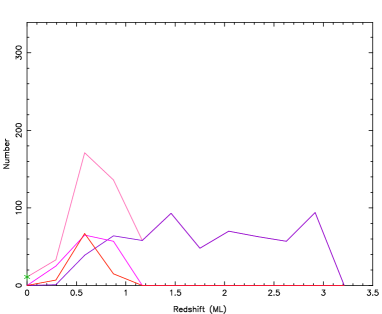 b)
b)