Luminosity Functions of Lyman-Break Galaxies at $z\sim 4$ and 5
in the Subaru Deep Field

Abstract

We investigate the luminosity functions of Lyman-break galaxies (LBG) at $z\sim 4$ and 5 based on the optical imaging data obtained in the Subaru Deep Field (SDF) Project, a program conducted by Subaru Observatory to carry out a deep and wide survey of distant galaxies. Three samples of LBGs in a contiguous 875 arcmin² area are constructed. One consists of LBGs at $z\sim 4$ down to $i^{\prime}=26.85$ selected with the $B\!-\!R$ vs $R\!-\!i^{\prime}$ diagram ($BRi^{\prime}$-LBGs). The other two consist of LBGs at $z\sim 5$ down to $z^{\prime}=26.05$ selected with two kinds of two-color diagrams: $V\!-\!i^{\prime}$ vs $i^{\prime}\!-\!z^{\prime}$  ($Vi^{\prime}z^{\prime}$-LBGs) and $R\!-\!i^{\prime}$ vs $i^{\prime}\!-\!z^{\prime}$ ($Ri^{\prime}z^{\prime}$-LBGs). The number detected is $3,808$ for $BRi^{\prime}$-LBGs, 539 for $Vi^{\prime}z^{\prime}$-LBGs, and 240 for $Ri^{\prime}z^{\prime}$-LBGs. The adopted selection criteria are proved to be fairly reliable by the spectroscopic observation of 63 LBG candidates, among which only 2 are found to be foreground objects. We estimate the fraction of contamination and the completeness for these three samples by Monte Carlo simulations, and derive the luminosity functions of the LBGs at rest-frame ultraviolet wavelengths down to $M_{\mathrm{UV}}=-19.2$ at $z\sim 4$ and $M_{\mathrm{UV}}=-20.3$ at $z\sim 5$. We find clear evolution of the luminosity function over the redshift range of $0\leq z\leq 6$, which is accounted for by a sole change in the characteristic magnitude, $M^{\ast}$. The cosmic star formation rate (SFR) density at $z\sim 4$ and $z\sim 5$ is measured from the luminosity functions. The measurements of the integrated SFR density at these redshifts are largely improved, since the luminosity functions are derived down to very faint magnitudes. We examine the evolution of the cosmic SFR density and its luminosity dependence over $0\leq z\lesssim 6$. The SFR density contributed from brighter galaxies is found to change more drastically with cosmic time. The contribution from galaxies brighter than $M^{\ast}_{\mathrm{z=3}}-0.5$ has a sharp peak around $z=3$ – 4, while that from galaxies fainter than $M^{\ast}_{\mathrm{z=3}}-0.5$ evolves relatively mildly with a broad peak at earlier epoch. Combining the observed SFR density with the standard Cold Dark Matter model, we compute the cosmic SFR per unit baryon mass in dark haloes, i.e., the specific SFR. The specific SFR is found to scale with redshift as $(1+z)^{3}$ up to $z\sim 4$, implying that the efficiency of star formation is on average higher at higher redshift in proportion to the cooling rate within dark haloes, while this is not simply the case at $z\gtrsim 4$.

1 INTRODUCTION

When and how galaxies formed is one of the primary questions in astronomy today. Observations of young galaxies at high redshifts are a straightforward approach to this problem. Over the past decade, it has become feasible to undertake large surveys of galaxies at high redshifts. What made this possible is the progress in observing technology including telescopes and detectors, and also sophistication of selection methods to locate high-redshift galaxies. Probably the most efficient method is the Lyman-break technique. It is a simple photometric technique based on the continuum features in rest-frame ultraviolet spectra redshifted into optical bandpasses, and requires only optical imaging in a few bandpasses. Pioneered by Guhathakurta et al. (1990), this method has been successfully used to find many young, star-forming galaxies beyond $z\sim 2$ (e.g., Steidel & Hamilton, 1992; Steidel et al., 1999; Lehnert & Bremer, 2003; Iwata et al., 2003; Ouchi et al., 2004; Dickinson et al., 2004; Sawicki & Thompson, 2006). Steidel et al. (2003) made spectroscopic observation for about 1000 photometrically selected $z\sim 3$ galaxies and verified the usefulness of this method. High-redshift galaxies selected by this method are called Lyman-break galaxies (LBGs).

Since their first discovery in the 1990s, various properties of LBGs have been extensively studied. One of the most fundamental measurements is the luminosity function (LF) at rest-frame ultraviolet wavelengths (i.e., the number density of galaxies as a function of ultraviolet luminosity). Besides providing information on the number density of galaxies, the LF can be used to probe the star formation activity in the universe, because ultraviolet luminosity is sensitive to star formation. Thus the ultraviolet luminosity density derived by integrating the LF is related to the star formation rate (SFR) density in the universe. By obtaining the LF at various redshifts and examining its evolution, one can gain insights into the formation history of galaxies and the star formation history in the universe.

Steidel et al. (1999) derived the LF at $z\sim 3$ from their large LBG sample, finding that their data are well fitted by a Schechter function with a low-luminosity slope $\alpha$ of $-1.6$ down to $L\simeq 0.1L^{\ast}$. They extended their LBG search to $z\sim 4$, to detect no significant evolution of the LF at bright magnitudes ($M<-21.1$) from $z\sim 4$ to $z\sim 3$. More recent observations have also derived the LF at $z\sim 4$ and $z\sim 5$ (Iwata et al., 2003; Ouchi et al., 2004; Gabasch et al., 2004; Sawicki & Thompson, 2006). The frontier of LBG searches now extends beyond $z\sim 5$. (Yan et al., 2003; Stanway et al., 2003; Bunker et al., 2004; Bouwens et al., 2004, 2005; Shimasaku et al., 2005).

However, it is not easy to construct a large sample of LBGs beyond $z\sim 4$ covering a wide range of absolute magnitude because of their apparent faintness and low surface number density. In the first place, most of the studies to date are limited to bright LBGs. Consequently, the shape of the faint end of the LF has not been well determined. Thus, the estimation of the cosmic SFR density has a considerably large uncertainty (about a factor of 3 – 10) due to the long extrapolation of the observed LFs to faint magnitudes (see Ouchi et al., 2004). Exploring LBGs down to faint luminosities is necessary in order to determine the overall shape of the LF, and to measure the cosmic SFR density accurately. Although some surveys are extremely deep, they are restricted to very small areas (e.g. $\sim 4$ arcmin² for the Hubble Deep Field, and $\sim 10$ arcmin² for the Hubble Ultra Deep Field). Surveys based on such a small area probably suffer from cosmic variance, i.e., inhomogeneities in the spatial distribution of LBGs. Although deep and wide surveys of LBGs at $z\sim 4$ have been made by Gabasch et al. (2004) and Sawicki & Thompson (2006) very recently, large samples for $z\gtrsim 4$ are still very limited. It is therefore crucial to construct a new LBG sample from a survey of a similar depth and width and derive the LF and the cosmic SFR independently.

In this paper, we present a detailed study of LBGs at $z\sim 4$ – 5 based on the deep and wide-field images obtained in the Subaru Deep Field (SDF) Project (Kashikawa et al., 2004). The SDF Project is a program conducted by Subaru Observatory to carry out a deep galaxy survey over a blank field as large as $\simeq 0.2$ square degree. Exploiting these unique data, we make the largest samples of LBGs at $z\sim 4$ and 5, and derive the LFs down to very faint magnitudes; $M_{\mathrm{UV}}=-19.2$ at $z\sim 4$ and $M_{\mathrm{UV}}=-20.3$ at $z\sim 5$. This extends the LBG search by Ouchi et al. (2004) based on shallower and smaller area data of the same field some $\sim 0.5$ mag further and $1.5$ times wider, leading to a $\sim 3$ times increase in number of LBGs detected. These samples enable us to examine the behavior of the LF more accurately over a wide magnitude range and obtain more reliable measurements of the cosmic SFR density in the early universe. The LFs of LBGs at $z\sim 4$ and 5 we derive are found to differ from those at the same redshift ranges obtained in some of the previous surveys.

Recently, the LF at ultraviolet wavelengths of present-day galaxies ($z\sim 0$) has been derived very accurately from a large galaxy survey by Galaxy Evolution Explorer (GALEX) (Wyder et al., 2005). Arnouts et al. (2005) have derived the LFs at $0.2\leq z\leq 1.2$ also based on GALEX observations. Measurements at $z\sim 6$ are now available (Bouwens et al., 2005; Shimasaku et al., 2005). Combining the results at $z\sim 4$ and 5 from this work with those at lower redshifts and $z\sim 6$ from the literature, we investigate the evolutionary history of galaxies in terms of the star formation activity over $0\leq z\lesssim 6$.

The outline of this paper is as follows. Section 2 describes the data of the SDF Project used in this study. Section 3 describes the selection of LBGs at $z\sim 4$ and 5 from the photometric data. The contamination by interlopers and the completeness of the samples are also estimated. In Section 4, the rest-frame UV luminosity functions of LBGs at $z\sim 4$ and 5 are derived, and compared with those by other authors. In Section 5 we discuss the evolution of the cosmic star formation activity over the redshift range $0\leq z\leq 6$. The evolution of the luminosity function and the cosmic star formation rate density is examined. Section 6 summarizes this study.

Throughout this paper, the photometric system is based on AB magnitude (Oke & Gunn, 1983). The cosmology adopted is a flat universe with $\mathrm{\Omega}_{m}=0.3$, $\mathrm{\Omega}_{\mathrm{\Lambda}}=0.7$, and a Hubble constant of $H_{0}=70$ km s^-1 Mpc^-1. These values are consistent with those obtained from the latest CMB observations (Spergel et al., 2003).

2 DATA

The data used in this study are obtained in the SDF Project (Kashikawa et al., 2004). The program consists of very deep multi-band optical imaging, NIR imaging for smaller portions of the field, and follow-up optical spectroscopy. This study is based on the optical imaging data together with additional information from the spectroscopic data. Full details of the optical imaging observations, data reduction, and object detection and photometry are described in Kashikawa et al. (2004).

2.1 Imaging Data

The optical imaging observations in the SDF Project were carried out with the prime-focus camera (Suprime-Cam: Miyazaki et al., 2002) mounted on the 8.2 m Subaru Telescope (Iye et al., 2004) in 2002 and 2003. The imaging was made for a single field of view of the Suprime-Cam ($34^{\prime}\times 27^{\prime}$) toward the Subaru Deep Field (SDF: Maihara et al., 2001), centered on [$13^{h}24^{m}38.^{s}9$, $+27^{\circ}29^{\prime}25.^{\prime\prime}9$ (J2000)]. The scale of the Suprime-Cam is $0.^{\prime\prime}202$ pixel^-1. The images were taken in five standard broad-bands filters: $B$, $V$, $R$, $i^{\prime}$, and $z^{\prime}$, and two narrow-bands filters: NB816 and NB921. The central wavelengths of the broad-bands are 4458 Å, 5478 Å, 6533 Å, 7684 Å, and 9037 Å for $B$, $V$, $R$, $i^{\prime}$, and $z^{\prime}$, respectively. The SDF was previously imaged during the commissioning runs of the Suprime-Cam in 2001 in five bandpasses, $B$, $V$, $R$, $i^{\prime}$, and $z^{\prime}$, with 1 – 3 hours exposure times. The work by Ouchi et al. (2004) is based on these data. They were co-added in constructing the final images.

All individual CCD data with good quality were reduced and combined to make a single image for each band using a pipeline software package (Ouchi, 2003) whose core programs were taken from IRAF and mosaic-CCD data reduction software (Yagi et al., 2002). The combined images for all seven bands were aligned and smoothed with Gaussian kernels so that all have the same seeing size, a PSF FWHM of $0.^{\prime\prime}98$. The efficiency and reliability of object detection and photometry in regions near the edges of the images are significantly lower on account of low $S/N$ ratios caused by dithering. Regions around very bright stars are also degraded due to bright haloes and saturation trails. We carefully defined these low-quality regions, and did not use objects located in these regions. The effective area of the final images after removal of the low-quality regions is 875 arcmin². Photometric calibration for the images was made using standard stars taken during the observations. The total exposure time reaches $\sim 10$ hours for each band, and the limiting magnitude ($3\sigma$ within a $2^{\prime\prime}$ diameter aperture) is 28.45 ($B$), 27.74 ($V$), 27.80 ($R$), 27.43 ($i^{\prime}$), 26.62 ($z^{\prime}$), 26.63 (NB816), and 26.54 (NB921).

Object detection and photometry were performed using SExtractor version 2.1.6 (Bertin & Arnouts, 1996). A collection of at least 5 contiguous pixels above the $2\sigma$ sky noise was identified as an object. The object detection was made for all seven images independently. For each of the objects detected in a given band image, photometry was made in all the images at exactly the same position as in the detection-band image. Thus, seven catalogs were constructed for respective detection bands. For the present study, we limit the catalogs to objects whose detection-band magnitudes are brighter than the $5\sigma$ limiting magnitude ($5\sigma$ sky noise within a $2^{\prime\prime}$ diameter aperture) of that band, in order to provide a reasonable level of photometric completeness. We use magnitudes within a $2^{\prime\prime}$ diameter aperture to derive the colors of objects, and adopt MAG_AUTO in SExtractor for total magnitudes. The magnitudes of objects were corrected for a small amount of foreground Galactic extinction toward the SDF using the dust map of Schlegel et al. (1998). Since the variation of $E(B-V)$ over the SDF of 875 arcmin² is at most 0.007, we adopt a single value, $E(B-V)=0.017$, for correction, which is the value at the center of the SDF. The value of $E(B-V)=0.017$ corresponds to an extinction of $A_{B}=0.07$, $A_{V}=0.05$, $A_{R}=0.04$, $A_{i^{\prime}}=0.03$, $A_{z^{\prime}}=0.02$, $A_{\mathrm{NB816}}=0.03$, and $A_{\mathrm{NB921}}=0.02$.

2.2 Spectroscopic Data

We carried out spectroscopic follow-up observations for some objects in our catalogs with the Subaru Faint Object Camera and Spectrograph (FOCAS: Kashikawa et al., 2002) on the Subaru Telescope during 2002 – 2004 and DEIMOS (Faber et al., 2003) on the Keck II Telescope in 2004. The spectroscopic observations were made in the multi-object slit mode. For the FOCAS observations, we used a 300 line mm^-1 grating with an O58 order-cut filter and an Echelle with a $z^{\prime}$ filter. Slit widths on the masks were either $0.^{\prime\prime}8$ or $0.^{\prime\prime}6$ for the 300 line configuration, resulting in a spectral resolution of 9.5 Å and 7.1 Å at 8150 Å, respectively, and $0.^{\prime\prime}8$ for the Echelle. The integration times of respective masks were 7000 – 9000 seconds. Flux calibration was made with spectra of the spectroscopic standard stars Hz 44 and Feige 34. The data were reduced in a standard manner. For the observations with DEIMOS, we used a 830 line mm^-1 grating with a GG495 order-cut filter. Slit widths were $1.^{\prime\prime}0$, which gave a spectral resolution of 3.97 Å. The integration times were 6300 – 19800 seconds. Spectra of the standard stars BD+28d4211 and Feige 110 were taken for flux calibration. The data were reduced with the spec2d pipeline for the reduction of DEEP2 DEIMOS data. In addition, we also use spectra of objects in the SDF which were taken during the guaranteed time observations of the FOCAS in 2001 (Kashikawa et al., 2003; Ouchi et al., 2004).

In Figures 1 and 2, we present the distribution of the $z^{\prime}$ magnitude of the spectroscopic objects and their redshift distribution, respectively. Only objects with $z_{\mathrm{spec}}<5.5$ are included here.

Figure 1: The magnitude distribution of the spectroscopic objects with $z_{\mathrm{spec}}<5.5$ in our catalogs.

Figure 2: The redshift distribution of the spectroscopic objects with $z_{\mathrm{spec}}<5.5$ in our catalogs.

3 LYMAN-BREAK GALAXY SAMPLES AT $z\sim 4$ AND $5$

3.1 Selection of Lyman-break Galaxies

We demonstrate the principle of the Lyman-break color selection technique to locate galaxies at $z\sim 4$ and $z\sim 5$ in Figure 3. For galaxies at $z\sim 4$, the break in the spectrum at rest-frame ultraviolet wavelength enters the $B$ band and the flat continuum longward of Lyman-$\alpha$ shifts to wavelengths longer than the $R$ band, and these galaxies are identified by their red $B\!-\!R$ color and blue $R\!-\!i^{\prime}$ color. We select LBGs at $z\sim 4$ by these two colors (hereafter called $BRi^{\prime}$-LBGs). For galaxies at $z\sim 5$, the spectral break enters into the $V$ band and the flat continuum is sampled at wavelengths longer than the $i^{\prime}$ band. At $z\sim 5$, the attenuation due to the Lyman-$\alpha$ forest is so strong that the flux in the $R$ band is severely suppressed, as well as the flux in the $V$ band. Thus, galaxies at $z\sim 5$ are identified by their red $V\!-\!i^{\prime}$ or $R\!-\!i^{\prime}$ color and blue $i^{\prime}\!-\!z^{\prime}$ color. We make two samples for LBGs at $z\sim 5$: one selected by $V\!-\!i^{\prime}$ and $i^{\prime}\!-\!z^{\prime}$ colors, and the other selected by $R\!-\!i^{\prime}$ and $i^{\prime}\!-\!z^{\prime}$ colors (hereafter called $Vi^{\prime}z^{\prime}$-LBGs and $Ri^{\prime}z^{\prime}$-LBGs, respectively).

Figure 3: Upper panel: The $B$, $R$, and $i^{\prime}$ bandpasses overplotted on the spectrum of a generic $z=4$ galaxy (thick line), illustrating the utility of color selection technique using these three bandpasses for locating $z\sim 4$ galaxies. Lower panel: The $V$, $R$, $i^{\prime}$, and $z^{\prime}$ bandpasses overplotted on the spectrum of a generic $z=5$ galaxy (thick line). The band sets of $Vi^{\prime}z^{\prime}$ and $Ri^{\prime}z^{\prime}$ work well to isolate $z\sim 5$ galaxies.

Figures 4 – 6 illustrate the predicted positions of high-redshift galaxies and foreground objects (lower-redshift galaxies and Galactic stars) in three two-color diagrams: $B\!-\!R$ vs $R\!-\!i^{\prime}$, $V\!-\!i^{\prime}$ vs $i^{\prime}\!-\!z^{\prime}$, and $R\!-\!i^{\prime}$ vs $i^{\prime}\!-\!z^{\prime}$. The solid lines in these figures indicate the tracks for model spectra of young star-forming galaxies for the redshift range $z>3$. The model spectrum was constructed using the stellar population synthesis code developed by Kodama & Arimoto (1997). For model parameters, an age of 0.1 Gyr, a Salpeter initial mass function, and a star-formation timescale of 5 Gyr were adopted, and reddening of $E(B-V)=0.16$ was applied using the dust extinction formula for starburst galaxies by Calzetti et al. (2000). These values reproduce the average rest-frame ultraviolet-optical spectral energy distribution of LBGs observed at $z\sim 3$ (Papovich et al., 2001). We also show the tracks for model spectra with reddening of $E(B-V)=0$ and $0.3$ for reference. The absorption due to the intergalactic medium was applied following the prescription by Madau (1995). The dotted, dashed, and dot-dashed lines delineate the tracks for model spectra of local elliptical, spiral, and irregular galaxies, respectively, redshifted from $z=0$ to $z=3$. These spectra were also constructed using the stellar population synthesis code by Kodama & Arimoto (1997), and redshifted without evolution. The asterisks denote the 175 Galactic stars of various types whose spectra are given by Gunn & Stryker (1983). The colors are calculated by convolving constructed model spectra of galaxies or given spectra of stars with the response functions of the Suprime-Cam filters. It can be seen that the model young star-forming galaxy moves nearly vertically from the origin in these two-color diagrams at $z>3$, namely it becomes redder in $B\!-\!R$, $V\!-\!i^{\prime}$, and $R\!-\!i^{\prime}$ colors, while keeping $R\!-\!i^{\prime}$, $i^{\prime}\!-\!z^{\prime}$, and $i^{\prime}\!-\!z^{\prime}$colors blue, as redshift increases, and that it shifts into a portion of the two-color space which is unpopulated by foreground objects. At $z>5$, the $R\!-\!i^{\prime}$ color does not become redder very much while $i^{\prime}\!-\!z^{\prime}$ color becomes redder in the $R\!-\!i^{\prime}$ vs $i^{\prime}\!-\!z^{\prime}$ diagram. These figures imply that LBGs at $z\sim 4$ and those at $z\sim 5$ can be well isolated from foreground objects in the $B\!-\!R$ vs $R\!-\!i^{\prime}$ diagram, and in the $V\!-\!i^{\prime}$ vs $i^{\prime}\!-\!z^{\prime}$ and $R\!-\!i^{\prime}$ vs $i^{\prime}\!-\!z^{\prime}$ diagrams, respectively. The most critical contamination is caused by elliptical galaxies at $z\sim 0.5$, which come close to high-redshift galaxies in these diagrams due to the 4000 Å break on their spectra.

Figure 4: $B\!-\!R$ vs $R\!-\!i^{\prime}$ diagram where the predicted colors of model galaxies and stars are illustrated. The three solid lines indicate the tracks for model spectra of young star-forming galaxies with reddening of $E(B-V)=0$, $0.16$, and $0.3$ (from left to right).

The redshift range is from $z=3$ to higher redshifts, and the circles on the track mark the redshift interval of 0.1. The dotted, dashed, and dot-dashed lines delineate the tracks for model spectra of local elliptical, spiral, and irregular galaxies, respectively, redshifted from $z=0$ to $3$ without evolution. The circles on each track mark $z=0$, $1$, and $2$. The asterisks represent the colors of 175 Galactic stars given by Gunn & Stryker (1983). The thick line indicates the boundary which we adopt for the selection of $BRi^{\prime}$-LBGs.

Figure 5: $V\!-\!i^{\prime}$ vs $i^{\prime}\!-\!z^{\prime}$ diagram where the predicted colors of model galaxies and stars are illustrated. Lines and symbols are the same as in Figure 4. The thick line indicates the boundary which we adopt for the selection of $Vi^{\prime}z^{\prime}$-LBGs.

Figure 6: $R\!-\!i^{\prime}$ vs $i^{\prime}\!-\!z^{\prime}$ diagram where the predicted colors of model galaxies and stars are illustrated. Lines and symbols are the same as in Figure 4. The thick line indicates the boundary which we adopt for the selection of $Ri^{\prime}z^{\prime}$-LBGs.

In Figures 7 – 9, we show the distribution of all the objects contained in the catalogs in the two-color diagrams. When the magnitude of an object in a non-detection band is fainter than the $1\sigma$ magnitude of the band, the $1\sigma$ magnitude is assigned to the object. Objects with spectroscopic redshifts are shown with colored symbols in these figures, where different colors mean different redshift bins. It is found that the colors of spectroscopically identified objects match fairly well with those of model galaxies with corresponding redshifts in Figures 4 – 6.

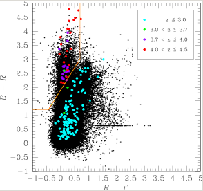
Figure 7: $B\!-\!R$ vs $R\!-\!i^{\prime}$ diagram for all the objects contained in the $i^{\prime}$-detection catalogs (106,025 objects down to $i^{\prime}\leq 26.85$). When the $B$ and/or $R$ magnitude of an object is fainter than the $1\sigma$ magnitude of the band, the $1\sigma$ magnitude is assigned to the object. The horizontal sequence along $\mbox{$B\!-\!R$}=0.62$ shows objects which are fainter than the $1\sigma$ magnitude in both $B$ and $R$.

The colored symbols show objects with spectroscopic redshifts, where cyan, green, violet, and red represent objects in the range $z<3.0$, $3.0\leq z<3.7$, $3.7\leq z<4.0$, and $4.0\leq z<4.5$, respectively. The thick orange line indicates the boundary which we adopt for the selection of $BRi^{\prime}$-LBGs.

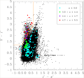
Figure 8: $V\!-\!i^{\prime}$ vs $i^{\prime}\!-\!z^{\prime}$ diagram for all the objects contained in the $z^{\prime}$-detection catalogs (76,351 objects down to $z^{\prime}\leq 26.05$). When the $V$ and/or $i^{\prime}$ magnitude of an object is fainter than the $1\sigma$ magnitude of the band, the $1\sigma$ magnitude is assigned to the object. The horizontal sequence along $\mbox{$V\!-\!i^{\prime}$}=0.29$ shows objects which are fainter than the $1\sigma$ magnitude in both $V$ and $i^{\prime}$.

The colored symbols show objects with spectroscopic redshifts, where cyan, green, violet, and red represent objects in the range $z<3.0$, $3.0\leq z<4.4$, $4.4\leq z<4.7$, and $4.7\leq z<5.5$, respectively. The thick orange line indicates the boundary which we adopt for the selection of $Vi^{\prime}z^{\prime}$-LBGs.

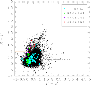
Figure 9: $R\!-\!i^{\prime}$ vs $i^{\prime}\!-\!z^{\prime}$ diagram for all the objects contained in the $z^{\prime}$-detection catalogs (76,351 objects down to $z^{\prime}\leq 26.05$). When the $R$ and/or $i^{\prime}$ magnitude of an object is fainter than the $1\sigma$ magnitude of the band, the $1\sigma$ magnitude is assigned to the object. The horizontal sequence along $\mbox{$R\!-\!i^{\prime}$}=0.35$ shows objects which are fainter than the $1\sigma$ magnitude in both $R$ and $i^{\prime}$.

The colored symbols show objects with spectroscopic redshifts, where cyan, green, violet, and red represent objects in the range $z<3.0$, $3.0\leq z<4.7$, $4.7\leq z<4.9$, and $4.9\leq z<5.5$, respectively. The thick orange line indicates the boundary which we adopt for the selection of $Ri^{\prime}z^{\prime}$-LBGs.

We adopt the same color criteria for $BRi^{\prime}$-LBGs and $Vi^{\prime}z^{\prime}$-LBGs as those of Ouchi et al. (2004). For $Ri^{\prime}z^{\prime}$-LBGs, we visually fine-tune their color criteria based on the increased redshift information. Specifically, we set the selection criteria for $BRi^{\prime}$-LBGs as:

$$B-R>1.2,$$

$$R-i^{\prime}<0.7,$$ (1)

$$B-R>1.6(R-i^{\prime})+1.9,$$

for $Vi^{\prime}z^{\prime}$-LBGs as:

$$V-i^{\prime}>1.2,$$

$$i^{\prime}-z^{\prime}<0.7,$$ (2a)

$$V-i^{\prime}>1.8(i^{\prime}-z^{\prime})+1.7,$$

$$B>3\sigma\ \mathrm{mag},$$ (2b)

and for $Ri^{\prime}z^{\prime}$-LBGs as:

$$R-i^{\prime}>1.0,$$

$$i^{\prime}-z^{\prime}<0.7,$$ (3a)

$$R-i^{\prime}>1.2(i^{\prime}-z^{\prime})+0.9,$$

$$B,\ V>3\sigma\ \mathrm{mag}.$$ (3b)

The boundaries on the two-color diagrams defined by these color criteria are outlined with the thick orange lines in Figures 4 – 6 and 7 – 9. For the bands which are placed entirely shortward of the Lyman break, we additionally require that LBGs should be non-detected ((2b) and (3b)), which is expected to work effectively to reduce contamination from foreground galaxies.

We apply these selection criteria to the catalogs. We use the $i^{\prime}$-detection catalogs for $BRi^{\prime}$-LBGs, which contain $106,025$ objects to a limit of $i^{\prime}=26.85$ (total magnitude corrected for the Galactic extinction), and the $z^{\prime}$-detection catalogs for $Vi^{\prime}z^{\prime}$-LBGs and $Ri^{\prime}z^{\prime}$-LBGs, which contain $76,351$ objects to $z^{\prime}=26.05$ (total magnitude corrected for the Galactic extinction). The number of objects which satisfy the selection criteria, i.e., the number of LBG candidates, is $3,808$ for $BRi^{\prime}$-LBGs, 539 for $Vi^{\prime}z^{\prime}$-LBGs, and 240 for $Ri^{\prime}z^{\prime}$-LBGs . Table 1 summarizes the samples of the LBG candidates.

The selection criteria are shown by our spectroscopy to be fairly reliable. We spectroscopically observed 105 objects in the $BRi^{\prime}$-LBG sample, and identified 42 objects. Among the 42, only one is an interloper at $z=3.29$, with the remaining 41 being at $z\geq 3.7$. Similarly, 32 objects from the $Vi^{\prime}z^{\prime}$-LBG sample were spectroscopically observed, and 23 were identified. All but one of the 23 objects are at $z\geq 4.4$; the remaining one appears to be a Galactic star. In the $Ri^{\prime}z^{\prime}$-LBG sample, 12 objects were spectroscopically observed, and 9 were identified. All are found to be at $z\geq 4.5$. Possible reasons for the low detection rate for $BRi^{\prime}$-LBGs are that the Ly$\alpha$ emission of $z\sim 4$ LBGs is on average weaker than that of $z\sim 5$ LBGs and that the Ly$\alpha$ line at $z\sim 4$ falls in the wavelength range where the sensitivity of our spectroscopy is relatively low. The failed sample may also include interlopers between $z\sim 2$ and $3$ whose strong line features do not enter the wavelength coverage of our spectrograph. From the following simulation, however, we infer that the fraction of such interlopers is not so high in our LBG sample. First, we add noise to the colors of all objects outside of the $BRi^{\prime}$ selection criteria in our photometric catalog according to their measured magnitudes. We then count the objects which now meet the selection criteria due to the modified colors, to find that they are less than $10\%$ of the original LBG candidates even for the faintest magnitude bin where photometric errors are the largest. Note that this simulation gives an upper limit to the fraction of interlopers, since the measured colors already include photometric errors. In Figure 10, we present the apparent magnitude distribution of the spectroscopically identified objects in each LBG sample. Although the targets of spectroscopy is biased toward bright objects, we emphasize here that the spectroscopic samples also include faint objects and there are no interlopers even among them. We cannot, however, rule out the possibility that there may be interlopers for which no redshift have been secured. Figure 11 shows the redshift distribution of the spectroscopic samples. The average redshift is $<z>_{\mathrm{spec}}=4.1$ for $BRi^{\prime}$-LBGs, $<z>_{\mathrm{spec}}=4.8$ for $Vi^{\prime}z^{\prime}$-LBGs, and $<z>_{\mathrm{spec}}=4.9$ for $Ri^{\prime}z^{\prime}$-LBGs. Examples of spectra of $z\sim 4$ LBGs and $z\sim 5$ LBGs are shown in Figures 12 and 13, respectively.

Table 1: Samples of LBG candidates

Sample Name	Number of Candidates	Detection Band	Magnitude Range
$BRi^{\prime}$-LBG	3,808	$i^{\prime}$	$i^{\prime}=22.85-26.85$
$Vi^{\prime}z^{\prime}$-LBG	0.539	$z^{\prime}$	$z^{\prime}=23.55-26.05$
$Ri^{\prime}z^{\prime}$-LBG	0.240	$z^{\prime}$	$z^{\prime}=24.05-26.05$

Figure 10: The magnitude distribution of the spectroscopically identified objects in each LBG sample. Dotted histograms show the magnitude distribution of all the objects in each LBG sample normalized to the number of the spectroscopically identified objects.

Figure 11: The redshift distribution of the spectroscopically identified objects in each LBG sample. Dotted lines show the redshift distribution functions from the Monte Carlo simulation (see §3.3) normalized to the number of the spectroscopically identified objects.

Figure 12: Examples of spectra of Lyman-break galaxies at $z\sim 4$ with good quality that have prominent spectral features such as a strong Ly$\alpha$ emission line and interstellar lines.

The lowest panel shows a relative night-sky spectrum.

Figure 13: Same as Figure 12, but for $z\sim 5$.

3.2 Number Counts

The observed number counts of the LBG candidates as a function of apparent magnitude are shown in Figures 14 – 16, along with those measured by other authors who selected similar LBGs. None of the data is corrected for contamination or incompleteness. Previous LBG surveys included in the figures are summarized in Table 2. Ouchi et al. (2004) used the same photometric systems to make samples of LBGs at $z\sim 4$ over a 543 arcmin² area and LBGs at $z\sim 5$ over a 616 arcmin² area of the SDF. Steidel et al. (1999) carried out a search for LBGs at $z\sim 4$ using $G\!-\!\mathfrak{R}$, $\mathfrak{R}\!-\!I$ colors in a total of 828 arcmin² area of 10 separate fields. Sawicki & Thompson (2006) undertake a survey of LBGs at $z\sim 4$ with the same photometric systems and selection criteria that Steidel et al. (1999) use but to a deeper magniude in the Keck Deep Fields which cover a total area of 169 arcmin² and consist of five fields. Iwata et al. (2003) found LBGs at $z\sim 5$ using $V\!-\!I_{c}$, $I_{c}\!-\!z^{\prime}$ colors in a 575 arcmin² area including the Hubble Deep Field North. Capak et al. (2004) obtained number counts of LBGs at $z\sim 4$ selected by $B\!-\!R$, $R\!-\!I_{c}$ colors and LBGs at $z\sim 5$ selected by $V\!-\!I_{c}$, $I_{c}\!-\!z^{\prime}$ colors from a 720 arcmin² area centered on the Hubble Deep Field North. Our limiting magnitudes are among the faintest ones in the LBG samples for $z\sim 4$ and 5 constructed to date.

Figure 14: Observed number counts of LBGs at $z\sim 4$ uncorrected for incompleteness or contamination. The filled circles represent the $BRi^{\prime}$-LBGs in this study. Comparison is made with the previous measurements obtained by Ouchi et al. (2004) (open circles), Steidel et al. (1999) (open squares), Sawicki & Thompson (2006) (open pentagons), and Capak et al. (2004) (crosses). The error bars for this study, Ouchi et al. (2004), and Capak et al. (2004) reflect Poisson errors. The error bars for Steidel et al. (1999) and Sawicki & Thompson (2006) include an estimate of cosmic variance from their multiple fields as well as Poisson errors.

Figure 15: Observed number counts of $V$-dropout LBGs at $z\sim 5$ uncorrected for incompleteness or contamination. The filled circles represent the $Vi^{\prime}z^{\prime}$-LBGs in this study. Comparison is made with the previous measurements obtained by Ouchi et al. (2004) (open circles), Iwata et al. (2003) (open triangles), and Capak et al. (2004) (crosses). The error bars reflect Poisson errors.

Figure 16: Observed number counts of $R$-dropout LBGs at $z\sim 5$ uncorrected for incompleteness or contamination. The filled circles represent the $Ri^{\prime}z^{\prime}$-LBGs in this study. Comparison is made with the previous measurements obtained by Ouchi et al. (2004) (open circles). The error bars reflect Poisson errors.

Table 2: LBG surveys in the literature

Sample	Area [arcmin2]	$m_{\mathrm{limit}}$			$N$	Selection	Fig. in this paper	Ref.
$z\sim 4$	0875	$i^{\prime}$	$=$	$26.85$	$3,808$	$B\!-\!R$, $R\!-\!i^{\prime}$	Fig. 14, 19, 21	This study
$z\sim 5$	0875	$z^{\prime}$	$=$	$26.05$	0.539	$V\!-\!i^{\prime}$, $i^{\prime}\!-\!z^{\prime}$	Fig. 15, 20, 21	This study
$z\sim 5$	0875	$z^{\prime}$	$=$	$26.05$	0.240	$R\!-\!i^{\prime}$, $i^{\prime}\!-\!z^{\prime}$	Fig. 16, 20, 21	This study
$z\sim 3$	1046	$\mathfrak{R}$	$=$	$25.5\phantom{0}$	$1,270$	$U_{n}\!-\!G$, $G\!-\!\mathfrak{R}$	Fig. 21. 00. 00	Steidel et al. (1999)
$z\sim 4$	0828	$I$	$=$	$25.0\phantom{0}$	00207	$G\!-\!\mathfrak{R}$, $\mathfrak{R}\!-\!I$	Fig. 14, 19. 00	Steidel et al. (1999)
$z\sim 4$	0543	$i^{\prime}$	$=$	$26.3\phantom{0}$	$1,438$	$B\!-\!R$, $R\!-\!i^{\prime}$	Fig. 14, 19. 00	Ouchi et al. (2004)
$z\sim 4$	0720	$I_{c}$	$=$	$25.5\phantom{0}$	?	$B\!-\!R$, $R\!-\!I_{c}$	Fig. 14. 00. 00	Capak et al. (2004)
$z\sim 4$	0169	$\mathfrak{R}$	$=$	$27.0\phantom{0}$	0.427	$G\!-\!\mathfrak{R}$, $\mathfrak{R}\!-\!I$	Fig. 19. 00. 00	Sawicki & Thompson (2006)
$z\sim 5$	0575	$I_{c}$	$=$	$25.95$	0.305	$V\!-\!I_{c}$, $I_{c}\!-\!z^{\prime}$	Fig. 15, 20. 00	Iwata et al. (2003)
$z\sim 5$	0616	$z^{\prime}$	$=$	$25.8\phantom{0}$	0.246	$V\!-\!i^{\prime}$, $i^{\prime}\!-\!z^{\prime}$	Fig. 15, 20. 00	Ouchi et al. (2004)
$z\sim 5$	0720	$I_{c}$	$=$	$25.5\phantom{0}$	?	$V\!-\!I_{c}$, $I_{c}\!-\!z^{\prime}$	Fig. 15. 00. 00	Capak et al. (2004)
$z\sim 5$	0616	$z^{\prime}$	$=$	$25.8\phantom{0}$	00.68	$R\!-\!i^{\prime}$, $i^{\prime}\!-\!z^{\prime}$	Fig. 16, 20. 00	Ouchi et al. (2004)
$z\sim 6$	0012	$z^{\prime}$	$=$	$29.5\phantom{0}$	0.506	$i\!-\!z$, $V\!-\!z$	Fig. 21. 00. 00	Bouwens et al. (2005)
$z\sim 6$	0767	$z_{\mathrm{R}}$	$=$	$25.4\phantom{0}$	00.12	$i^{\prime}\!-\!z_{\mathrm{R}}$, $z_{\mathrm{B}}\!-\!z_{\mathrm{R}}$	Fig. 21. 00. 00	Shimasaku et al. (2005)

In general, number counts measurements of LBGs are dependent on detection completeness, photometric systems used, and selection criteria. It is found that our counts match very well with those of Ouchi et al. (2004) for all the samples except for brightest bins. While we use MAG_AUTO in SExtractor as total magnitudes of objects, Ouchi et al. (2004) calculate total magnitudes from aperture magnitudes through a fixed aperture correction of $-0.2$ mag. The correction value, however, actually can range to as much as $-0.4$ mag for bright LBGs. A shift of the magnitudes of Ouchi et al. (2004) by $-0.2$ mag ($=-0.4-(-0.2)$) can settle the disagreement between Ouchi et al.’s (2004) and our counts. The counts of Capak et al. (2004) are lower than our counts for $z\sim 4$ widely at faint magnitudes and for $z\sim 5$ at the faintest magnitude of Capak et al. (2004). The lower detection completeness of their data might be a major cause of this inconsistency; the $5\sigma$ limiting magnitude of their data is about 1 mag brighter than that of the SDF Project data. For $z\sim 4$ LBGs, our measurements agree with those of Steidel et al. (1999), although Steidel et al.’s (1999) measurements are limited to objects brighter than 25 mag. At faint magnitudes, however, our measurements are higher than those of Sawicki & Thompson (2006). For $z\sim 5$ LBGs, over a wide range of bright magnitudes ($m<25$), a discrepancy is found between the counts of Iwata et al. (2003) and either ours or those of Capak et al. (2004) who surveyed almost the same field as Iwata et al. (2003); Iwata et al.’s (2003) counts are higher about a factor of 3 – 10. The selection criteria of Iwata et al. (2003) are somewhat looser than ours. Therefore, as Ouchi et al. (2004) and Capak et al. (2004) claim, the LBG sample of Iwata et al. (2003) could be strongly contaminated by foreground galaxies.

3.3 Completeness

The completeness at a given apparent magnitude and redshift is defined as the ratio of LBGs which are detected and also pass the selection criteria, to all the LBGs with the given apparent magnitude and redshift actually present in the universe. In general, completeness decreases as apparent magnitude goes fainter and as redshift goes away from the central redshift of the sample. The completeness of each LBG sample is estimated as functions of apparent magnitude and redshift through a Monte Carlo simulation.

In the simulation, we generate artificial LBGs over an apparent magnitude range of $23.1\leq m_{i^{\prime}}\leq 26.6$ for $BRi^{\prime}$-LBGs and $23.8\leq m_{z^{\prime}}\leq 25.8$ for $Vi^{\prime}z^{\prime}$-LBGs and $Ri^{\prime}z^{\prime}$-LBGs with an interval of $\Delta m=0.5$, and over a redshift range of $z=3.0\leq z\leq 5.9$ with an interval of $\Delta z=0.1$. All LBGs are assumed to have the same intrinsic spectrum described in §3.1, but with values of $E(B-V)=0.0$, $0.1$, $0.2$, $0.3$, and $0.4$. Thus, $1,200$ ($8\times 30\times 5$) objects for $BRi^{\prime}$-LBGs and $750$ ($5\times 30\times 5$) objects for $Vi^{\prime}z^{\prime}$-LBGs and $Ri^{\prime}z^{\prime}$-LBGs are generated. We assume that the shape of LBGs is PSF-like and assign apparent sizes to the artificial LBGs so that their size distribution measured by SExtractor (the peak FWHM is $\approx 1.^{\prime\prime}00-1.^{\prime\prime}04$) matches that of the observed LBG candidates. The artificial LBGs are then distributed randomly on the original images after adding Poisson noise according to their magnitudes, and object detection and photometry are performed in the same manner as done for real objects. A sequence of these processes is repeated 100 times to obtain statistically accurate values of completeness. In the simulation, the completeness for a given apparent magnitude, redshift, and $E(B-V)$ value can be defined as the ratio in number of the simulated LBGs which are detected and also satisfy the selection criteria, to all the simulated objects with the given magnitude, redshift, and $E(B-V)$ value. We calculate the completeness of the LBG samples by taking a weighted average of the completeness for each of the five $E(B-V)$ values. The weight is taken using the $E(B-V)$ distribution function of $z\sim 4$ LBGs derived by Ouchi et al. (2004)(open histogram in the bottom panel of their Fig.20), which is corrected for incompleteness due to selection biases. We plot the recovered artificial objects in the two-color diagrams by taking the number of objects with each $E(B-V)$ value according to the adopted $E(B-V)$ distribution function. We verify that the distribution well resemble that of real objects. Hence, our modeling is reasonably realistic. The resulting completeness, $p(m,z)$, is shown in Figure 17.

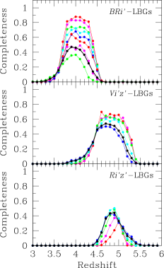
Figure 17: Completeness against the redshift of objects with different apparent magnitude for our LBG samples. In the panel of $BRi^{\prime}$-LBGs, the red, magenta, green, cyan, blue, red, magenta, and green (from top to bottom) lines denote the completeness for $i^{\prime}=23.45$, 23.95, 24.45, 24.95, 25.45, 25.95, 26.45, and 26.95, respectively. In the panels of $Vi^{\prime}z^{\prime}$-LBGs and $Ri^{\prime}z^{\prime}$-LBGs, the red, magenta, green, cyan, and blue lines denote the completeness for $z^{\prime}=24.15$, 24.65, 25.15, 25.65, and 26.15, respectively. The thick black lines in all panels indicate the magnitude-weighted completeness.

In order to examine the uniformity of completeness over our images, we split the images into two regions (a center region and a periphery region), each with the same area, and recalculate the completeness for each region. The non-uniformity is found to be small; the variation between the center region and the periphery region is within 10 %.

For each of the three LBG samples, magnitude-weighted redshift distribution functions are derived from $p(m,z)$ (thick black lines in Figure 17) by averaging the magnitude-dependent completeness weighted by the number of LBGs in each magnitude bin. The average redshift, $\bar{z}$, and its standard deviation, $s_{z}$, are calculated to be $\bar{z}=4.0$ and $s_{z}=0.3$ for $BRi^{\prime}$-LBGs, $\bar{z}=4.7$ and $s_{z}=0.3$ for $Vi^{\prime}z^{\prime}$-LBGs, and $\bar{z}=4.9$ and $s_{z}=0.2$ for $Ri^{\prime}z^{\prime}$-LBGs. We also compute magnitude-weighted redshift distribution functions where the weighting is done by the number of spectroscopically identified LBGs (dotted lines in Figure 11), to obtain the average redshift of $\bar{z}_{\mathrm{spec}}=4.0$ for $BRi^{\prime}$-LBGs, $\bar{z}_{\mathrm{spec}}=4.8$ for $Vi^{\prime}z^{\prime}$-LBGs, and $\bar{z}_{\mathrm{spec}}=4.9$ for $Ri^{\prime}z^{\prime}$-LBGs. These distribution functions are consistent with the redshift distributions of spectroscopic samples shown in Figure 11.

Although the above modeling well reproduces the observed distribution of objects in the two-color diagrams and the observed redshift distribution functions, we further explore to what extent the results would be affected by adopting different models. To begin with, we recalculate the completeness using model spectra with two other ages, 0.01 Gyr and 0.5 Gyr, to find that the completeness changes only a few percent. Then, we examine two extreme cases of dust extinction that all model spectra have $E(B-V)=0.0$ and 0.4. Changes in completeness are found to be negligibly small in either case except for $Ri^{\prime}z^{\prime}$-LBGs. Next, we examine the effect of changing the absorption by the intergalactic medium. If we shift the amount of attenuation to $\pm 1\sigma$ from the average amount given in Madau (1995), we obtain quite different completeness values. However, the redshift distribution functions derived are unrealistic, because they are strongly inconsistent with the distributions of spectroscopic objects. We also adopt Meiksin (2006)’s prescription for absorption by the intergalactic medium, to find completeness values similar to those based on Madau (1995)’s.

3.4 Contamination by Interlopers

We estimate the fraction of low-redshift interlopers in the LBG samples by a Monte Carlo simulation as follows. For the boundary redshift, $z_{0}$, between interlopers and LBGs, $z_{0}=3.5$ is adopted for $BRi^{\prime}$-LBGs, $z_{0}=4.0$ for $Vi^{\prime}z^{\prime}$-LBGs, and $z_{0}=4.5$ for $Ri^{\prime}z^{\prime}$-LBGs.

We use objects in the Hubble Deep Field North (HDFN), for which best-fit spectra and photometric redshifts are given by Furusawa et al. (2000), as a template of the color, magnitude, and redshift distribution of foreground galaxies, and generate 929 artificial objects which mimic the HDFN objects. The apparent sizes of the artificial objects are adjusted so that the size distribution recovered from the simulation is similar to that of the real objects in our catalogs. We distribute the artificial objects randomly on the original images after adding Poisson noise according to their magnitudes, and perform object detection and photometry in the same manner as employed for real objects. A sequence of these processes is repeated 100 times. In the simulation, the number of interlopers can be defined as the number of the simulated objects with low redshift ($z<z_{0}$) which are detected and also satisfy the selection criteria for LBGs. The number of interlopers expected in an LBG sample can then be calculated by multiplying the raw number by a scaling factor which corresponds to the ratio of the area of the SDF (875 arcmin²) to the area of the HDFN multiplied by the repeated times (100 $\times$ 3.92 arcmin²). Figure 18 shows the fraction of interlopers for our LBG samples as a function of magnitude. For the $BRi^{\prime}$-LBG and $Ri^{\prime}z^{\prime}$-LBG samples, the fraction is found to be less than 5% at any magnitude. For the $Vi^{\prime}z^{\prime}$-LBG sample, the contamination is higher but at most $\simeq 20$%. Most of the interlopers are in the redshift range of $0.2\leq z\leq 0.8$, as predicted from Figures 4 – 6. The rest are objects at redshifts which are close to the boundary redshift of each sample. The fraction of interlopers only at low redshifts (i.e., not at near the boundary redshifts) for each whole sample is around 1% for the $BRi^{\prime}$-LBG and $Ri^{\prime}z^{\prime}$-LBG samples, and around 9% for the $Vi^{\prime}z^{\prime}$-LBG sample.

The number density and the redshift distribution of galaxies in the HDFN may be largely different from the cosmic averages because the HDFN is a very small field. However, the contamination by interlopers for each of the three LBG samples calculated above is very low. We therefore expect that the uncertainty in contamination due to a possible (large) cosmic variance in the HDFN galaxies will not be a significant source of the error in the luminosity functions of LBGs derived in the next section.

Figure 18: Fraction of interlopers as a function of magnitude for our LBG samples.

4 LUMINOSITY FUNCTIONS AT REST-FRAME ULTRAVIOLET WAVELENGTHS

We derive the luminosity functions (LFs) of LBGs at $z\sim 4$ – 5 by applying the “effective volume” method (Steidel et al., 1999). The Monte Carlo simulation in §3.3 yields the effective survey volume as a function of apparent magnitude,

$$V_{\mathrm{eff}}(m) = \int_{z_{0}}^{\infty}p(m,z)\frac{dV(z)}{dz}\,dz,$$ (4)

where $p(m,z)$ is the probability that a galaxy of apparent magnitude $m$ at redshift $z$ is detected and passes the selection criteria (i.e., the completeness in §3.3 for magnitude $m$ and redshift $z$), $\frac{dV(z)}{dz}$ is the differential comoving volume at redshift $z$ for a solid angle of the surveyed area (875 arcmin²), and $z_{0}$ is the boundary redshift between low-redshift galaxies and LBGs. The effective volume obtained for each magnitude bin is provided in Tables 3 – 5.

Table 3: Number of LBGs detected, number of interlopers, and effective survey volume for $BRi^{\prime}$-LBGs.

Magnitude Range ($i^{\prime}$)	$N_{\mathrm{raw}}$	$N_{\mathrm{interloper}}$	$V_{\mathrm{eff}}$
22.85 – 23.35	0003	00.0	$1.74\times 10^{6}$
23.35 – 23.85	0012	00.0	$1.63\times 10^{6}$
23.85 – 24.35	0068	00.0	$1.49\times 10^{6}$
24.35 – 24.85	0231	00.0	$1.39\times 10^{6}$
24.85 – 25.35	0447	00.0	$1.22\times 10^{6}$
25.35 – 25.85	0763	08.9	$1.15\times 10^{6}$
25.85 – 26.35	1093	24.6	$8.77\times 10^{5}$
26.35 – 26.85	1191	26.8	$5.70\times 10^{5}$

Table 4: Number of LBGs detected, number of interlopers, and effective survey volume for $Vi^{\prime}z^{\prime}$-LBGs.

Magnitude Range ($z^{\prime}$)	$N_{\mathrm{raw}}$	$N_{\mathrm{interloper}}$	$V_{\mathrm{eff}}$
23.55 – 24.05	001	00.0	$1.34\times 10^{6}$
24.05 – 24.55	012	00.0	$1.31\times 10^{6}$
24.55 – 25.05	056	00.0	$1.31\times 10^{6}$
25.05 – 25.55	152	29.0	$1.17\times 10^{6}$
25.55 – 26.05	318	22.3	$9.66\times 10^{5}$

Table 5: Number of LBGs detected, number of interlopers, and effective survey volume for $Ri^{\prime}z^{\prime}$-LBGs.

Magnitude Range ($z^{\prime}$)	$N_{\mathrm{raw}}$	$N_{\mathrm{interloper}}$	$V_{\mathrm{eff}}$
24.05 – 24.55	003	0.0	$3.32\times 10^{5}$
24.55 – 25.05	018	0.0	$4.60\times 10^{5}$
25.05 – 25.55	066	2.2	$5.54\times 10^{5}$
25.55 – 26.05	153	2.2	$5.69\times 10^{5}$

The number density of LBGs corrected for incompleteness and contamination is computed as:

$$\phi(m) = \frac{N_{\mathrm{raw}}(m)-N_{\mathrm{interloper}}(m)}{V_{\mathrm{eff}}(m)},$$ (5)

where $N_{\mathrm{raw}}(m)$ and $N_{\mathrm{interloper}}(m)$ are the number of LBGs detected and the number of interlopers which is estimated from the simulations, respectively, in an apparent magnitude bin of $m$. Tables 3 – 5 also give $N_{\mathrm{raw}}(m)$ and $N_{\mathrm{interloper}}(m)$.

The number densities of LBGs in faint bins, especially the faintest bins, could be largely overestimated owing to Eddington bias from objects in fainter bins and/or beyond the limiting magnitude of the sample which have very large photometric errors and probably have a larger number density. We evaluate the effect of this bias for each LBG sample as follows. First, we construct a deeper sample of LBGs down to a magnitude limit fainter by 0.5 mag than the original value (for example, the new limit is $i^{\prime}\leq 27.35$ for $BRi^{\prime}$-LBGs). Then, using this deeper sample, we carry out Monte Carlo simulations similar to those made in §3.3, and derive $V_{\rm eff}(m)$ to calculate $\phi(m)$ to a deeper magnitude. From the simulations, we compute for each magnitude bin the fractions of LBGs which scatter out to other magnitude bins. Finally, we recalculate $\phi(m)$ by correcting the original number densities for the scatter along the magnitude axis. The number density of LBGs derived in this way is found to be consistent with the original calculation within statistical errors, down to the original limiting magnitude. This means that Eddington bias is negligibly small for our samples.

The LF in the rest-frame ultraviolet ($\simeq 1500$ Å) absolute magnitude, $M_{\mathrm{UV}}$, is obtained by converting $\phi(m)$ into $\phi(M_{\mathrm{UV}}(m))$. For each LBG sample, we calculate the absolute magnitude of LBGs from their apparent magnitude using the average redshift of the sample by

$$M_{\mathrm{UV}} = m+2.5\log(1+\bar{z})-5\log\left(d_{L}(\bar{z})\right)+5$$ (6)

$${}+(m_{\mathrm{UV}}-m),$$

where $d_{L}$ is the luminosity distance in units of pc. For apparent magnitude, $m$, we use $i^{\prime}$ magnitude for $BRi^{\prime}$-LBGs, and $z^{\prime}$ magnitude for $Vi^{\prime}z^{\prime}$-LBGs and $Ri^{\prime}z^{\prime}$-LBGs. The last term of Eq.6, $(m_{\mathrm{UV}}-m)$, is the difference between the magnitude at rest-frame 1500A and the magnitude in the bandpass being considered in the rest-frame. Using the representative galaxy models given in §3.1, we find $(m_{\mathrm{UV}}-m)$ to be negligible, or no larger than $0.03$ mag, over the redshift ranges selected by the color selection criteria we adopt. Thus we set $(m_{\mathrm{UV}}-m)$ to zero in Eq. 6. We assume that all of the LBGs have the average redshift of the sample. Indeed, for each of the three LBG samples, varying the redshift of an object over the standard deviation of the redshift distribution of the sample changes its absolute magnitude by not more than $0.1$ mag.

In Figures 19 and 20, the LFs at $z\sim 4$ and $z\sim 5$ are plotted respectively, along with those of other authors (See Table 2.). Note that Capak et al. (2004) do not derive the LFs. Our LFs are in excellent agreement with those of Ouchi et al. (2004) up to their faintest magnitudes for both redshifts. This agreement appears reasonable, since Ouchi et al. (2004) and this study are based on the same field (the SDF) and adopt almost the same selection criteria. Our LFs reach fainter magnitudes than theirs. However, there is a discrepancy between our $z\sim 4$ LF and that of Sawicki & Thompson (2006) in the Keck Deep Fields at the faint end; the faint-end slope of our LF is steeper than that of Sawicki & Thompson (2006). Gabasch et al. (2004) also derived the galaxy LFs at rest-frame ultraviolet wavelengths in the FORS Deep Field using photometric redshifts and obtained a similar result to that of Sawicki & Thompson (2006). The reason for this inconsistency is not clear. We note, however, that our raw counts before the correction of incompleteness already exceed the Sawicki & Thompson’s (2006) corrected counts, and thus that our higher values are not due to overcorrections. Additionally, our data have a sky coverage five times larger than that of the total of the five Keck Deep Fields. Thus, our LF is more robust against a possible cosmic variance on large scales, although the five separate Keck Deep Fields are less affected by cosmic variance than a single continuous field of the same sky coverage. At $z\sim 5$, our LF is different from that of Iwata et al. (2003) at bright magnitudes. One possible explanation for this difference is that Iwata et al. (2003) may select a large number of contaminants as mentioned in §3.2, resulting in the higher number density of bright LBGs.

Figure 19: UV luminosity functions (LFs) of LBGs at $z\sim 4$. Our data are shown by the filled circles. The open circles, open squares, and crosses are from Ouchi et al. (2004), Steidel et al. (1999), and Sawicki & Thompson (2006), respectively. The error bars for our data and Ouchi et al.’s (2004) reflect Poisson errors, and those for the other two data include both Poisson errors and an estimate of field-to-field variance from their multiple fields.

Figure 20: UV luminosity functions (LFs) of LBGs at $z\sim 5$. Our data from $Vi^{\prime}z^{\prime}$-LBG sample and $Ri^{\prime}z^{\prime}$-LBG sample are shown by the filled circles and filled triangles, respectively. The open circles and open triangles are from Ouchi et al.’s (2004) $Vi^{\prime}z^{\prime}$-LBG sample and $Ri^{\prime}z^{\prime}$-LBG sample, respectively. The crosses are from Iwata et al. (2003). The error bars reflect Poisson errors.

We find a good agreement between our $z\sim 5$ LFs obtained from the $Vi^{\prime}z^{\prime}$-LBG sample and the $Ri^{\prime}z^{\prime}$-LBG sample. The redshift ranges of these two samples are almost the same. This consistency in the results from the two independent manners provides strong support for LFs we obtained. As the $Vi^{\prime}z^{\prime}$-LBG sample contains a statistically larger number of objects and has higher completeness, we only use results from the $Vi^{\prime}z^{\prime}$-LBG sample in the following analysis for $z\sim 5$. These LFs obtained at $z\sim 4$ and 5 are found to be well reproduced by a semi-analytic model combined with high-resolution N-body simulations (Nagashima et al., 2005) when the observational selection effects are taken into account. We should, however, point out that the Lyman-break technique cannot select all star-forming galaxies at targeted redshifts. On the basis of spectroscopy of galaxies in an optically-selected, flux-limited sample, Le Fevre et al. (2005) claim that a large fraction of galaxies at $z\sim 3$ – 4 lie outside the selection boundaries for LBGs in two-color diagrams. In addition, submm-selected galaxies (e.g., Smail, Ivison, & Blain, 1997) and NIR-selected star-forming galaxies (e.g., Franx et al., 2003) are often too faint in optical wavelengths to be selected as LBGs, because of strong absorption by dust. Such dusty star-forming galaxies could contribute to the cosmic SFR density as much as do LBGs (e.g., Chapman et al., 2005). Therefore, the far UV luminosity function and the star formation rate density derived in this paper are for galaxies with modest dust extinction and passing selection criteria for LBGs, and thus they may be greatly modified if all star-forming galaxies are included.

We fit the LFs with the Schechter function (Schechter, 1976):

$$\phi(L)dL$$ (7)

$$= \phi^{\ast}\left(\frac{L}{L^{\ast}}\right)^{\alpha}\exp\left(-\frac{L}{L^{\ast}}\right)d\left(\frac{L}{L^{\ast}}\right),$$

or expressed in terms of absolute magnitude:

$$\phi(M_{\mathrm{UV}})dM_{\mathrm{UV}}$$ (8)

$$= \left(\frac{\ln 10}{2.5}\phi^{\ast}\right)\left(10^{-0.4(M_{\mathrm{UV}}-M_{\mathrm{UV}}^{\ast})}\right)^{\alpha+1}$$

$$\times\exp\left(-10^{-0.4(M_{\mathrm{UV}}-M_{\mathrm{UV}}^{\ast})}\right)dM_{\mathrm{UV}},$$

where $\phi^{\ast}$, $L^{\ast}$ ($M_{\mathrm{UV}}^{\ast}$), and $\alpha$ are parameters to be determined from the data. The parameter $\phi^{\ast}$ is a normalization factor which has a dimension of number density, $L^{\ast}$ is a “characteristic luminosity” (with an equivalent “characteristic absolute magnitude”, $M_{\mathrm{UV}}^{\ast}$), and $\alpha$ gives the slope of the luminosity function at the faint end. For the $z\sim 5$ LF, whose $\alpha$ has a rather large uncertainty, we evaluate $\phi^{\ast}$ and $M_{\mathrm{UV}}^{\ast}$ with $\alpha$ fixed to the best-fit value for the $z\sim 4$ LF, besides fitting with all three parameters left free. The best-fit parameters obtained are listed in Table 6.

Table 6: Luminosity function parameters

Sample Name	$\bar{z}$	$s_{z}$	$\phi^{\ast}$ [Mpc-3]	$M_{\mathrm{UV}}^{\ast}$	$\alpha$
$BRi^{\prime}$-LBGs	4.0	0.3	$1.46^{+0.41}_{-0.35}\times 10^{-3}$	$-21.14^{+0.14}_{-0.15}$	$-1.82^{+0.09}_{-0.09}$
$Vi^{\prime}z^{\prime}$-LBGs	4.7	0.3	$0.58^{+1.04}_{-0.49}\times 10^{-3}$	$-21.09^{+0.54}_{-0.74}$	$-2.31^{+0.68}_{-0.60}$
$Vi^{\prime}z^{\prime}$-LBGs	4.7	0.3	$1.23^{+0.44}_{-0.27}\times 10^{-3}$	$-20.72^{+0.16}_{-0.14}$	$-1.82$ (fixed)

5 EVOLUTION OF THE COSMIC STAR FORMATION ACTIVITY OVER $0\leq z\leq 6$

5.1 Evolution of the Luminosity Function

We plot the LFs at $z\sim 4$ and 5 obtained in this study with those of LBGs at $z\sim 3$ (Sawicki & Thompson, 2006) and $z\sim 6$ (Bouwens et al. 2004a; Shimasaku et al. 2005 from observation of the SDF in new filters sensitive to $\simeq 1\ \mu$m) in Figure 21. The LFs of UV (1500Å)-selected galaxies at $z\sim 0$ (Wyder et al., 2005) and $z\sim 1$ (Arnouts et al., 2005) are presented as well for reference. Figure 21 reveals clear evolution of the LF beyond $z\sim 4$. From $z\sim 4$ to $z\sim 3$, we find no significant evolution over the whole luminosity range. Sawicki & Thompson (2006) and Gabasch et al. (2004) detect an increase in faint galaxies across this redshift interval, but such an increase is not seen in our data. At lower redshifts, luminous galaxies strongly decrease in number from $z\gtrsim 2$ to $z\sim 0$, as has been found by previous studies.

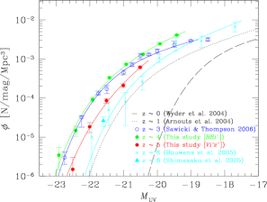
Figure 21: UV luminosity functions (LFs) of LBGs at $z\sim 3$ (blue open circles: Sawicki & Thompson, 2006),

$z\sim 4$ (green filled circles: this study [$BRi^{\prime}$-LBGs]), $z\sim 5$ (red filled circles: this study [$Vi^{\prime}z^{\prime}$-LBGs]), and $z\sim 6$ (cyan crosses: Bouwens et al. 2005; cyan filled triangle: Shimasaku et al. 2005). The error bars reflect Poisson errors. The best-fit Schechter function is also shown with the solid line for each data set except for that of Shimasaku et al. (2005). The black dashed line and the black dotted line indicate the LFs of UV-selected galaxies at $z\sim 0$ (Wyder et al., 2005), and $z\sim 1$ (Arnouts et al., 2005), respectively.

It is unlikely that the evolution in LF seen in Figure 21 is caused by the differences in selection criteria among the different samples. We find, using spectra of model galaxies, that the criteria for LBGs at $z\sim 3$, 4, and 5 select galaxies over similar ranges of age and $E(B-V)$. Since $i^{\prime}$-dropout galaxies at $z\sim 6$ are selected with $i^{\prime}-z^{\prime}$ color alone, they can have a wide range of $E(B-V)$. However, since no observation has reported a significant increase in dust extinction at $z>5$, it is reasonable to assume that the $i^{\prime}$-dropout galaxies are a similar population to LBGs at lower redshifts. Galaxies at $z\lesssim 1$ are selected in completely different ways from the Lyman-break technique. However, the differences in LF between $z\gtrsim 3$ and $z\lesssim 1$ seen in Figure 21 appear to be too large to be accounted for by possible selection effects. The dimming of LF seen for $z\lesssim 1$ will at least be qualitatively correct.

Figure 22 shows the evolution of Schechter parameters over $0\leq z\leq 6$. The filled circles represent our measurements. The other symbols show measurements taken from the literature. Note that the measurements at $z\sim 2$ and $z\sim 3$ from Arnouts et al. (2005) may have large uncertainties, because they are based solely on the HDFs which cover only a tiny area. The normalization factor, $\phi^{\ast}$, and the faint-end slope, $\alpha$, appear to be almost constant over the redshift range of $0.5\leq z\lesssim 6$, followed by a significant change at lower redshifts. We note that $\alpha$ at $z\sim 5$ is fixed to the value at $z\sim 4$ in evaluating the other two parameters but the value at $z\sim 4$ is similar to that at $z\sim 6$. From $z\sim 0.5$ to $z\sim 0$, $\phi^{\ast}$ rises by a half order of magnitude and $\alpha$ becomes shallower from $-1.6$ to $-1.2$. On the other hand, the characteristic magnitude, $M^{\ast}$, strongly and non-monotonically evolves over $0\leq z\leq 6$. It brightens by about 1 mag from $z\sim 6$ to $z\sim 4$, remains unchanged to $z\sim 3$, and then a significant fading of about 3 mag occurs from $z\sim 3$ to $z\sim 0$. In other words, the evolution of the LF seen in Figure 21 is accounted for by a change in $M^{\ast}$ with cosmic time. We point out, however, that there are different results about the LFs at $z\sim 4$ and $z\sim 5$, as mentioned in §4. Some groups claim that the faint-end slope is shallower at higher redshifts (Iwata et al., 2003; Gabasch et al., 2004; Sawicki & Thompson, 2006). The characteristic magnitude of Sawicki & Thompson (2006) at $z\sim 4$ is consistent with ours. Iwata et al. (2003) obtained an about 1 mag brighter value at $z\sim 5$ than ours.

Figure 22: Evolution of the luminosity function parameters with time. The filled circles represent the measurements from this study. The other symbols show measurements taken from the literature: open squares from Wyder et al. (2005), filled squares from Arnouts et al. (2005; GALEX), filled triangles from Arnouts et al. (2005; HDF), open circles from Sawicki & Thompson (2006), and crosses from Bouwens et al. (2005). For $z\sim 5$, we fixed $\alpha$ to the value at $z\sim 4$ ($\alpha=-1.82$) in evaluating the other two parameters.

5.2 Cosmic Star Formation Rate Density

5.2.1 Cosmic Star Formation Rate Density beyond $z\sim 3$

The ultraviolet luminosity density, $\rho_{L}$, at $z\sim 4$ and 5 is derived by integrating the LFs obtained in §4 as:

$$\rho_{L} = \int^{\infty}_{L_{\mathrm{min}}}L\,\phi(L)\,dL.$$ (9)

We consider two kinds of luminosity density. One is the “observed” luminosity density, $\rho_{L}^{\mathrm{obs}}$, which is derived from integration down to the faintest luminosity of the sample, $L_{\mathrm{min}}=L_{\mathrm{min}}^{\mathrm{obs}}$. This quantity, $\rho_{L}^{\mathrm{obs}}$, gives a lower limit of the true luminosity density. The faintest absolute magnitude of the sample at each redshift is $M_{\mathrm{UV}}=-19.2$ for $z\sim 4$ ($BRi^{\prime}$-LBGs) and $M_{\mathrm{UV}}=-20.3$ for $z\sim 5$ ($Vi^{\prime}z^{\prime}$-LBGs). The other is the luminosity density derived by integrating the LFs down to the same luminosity limit for all the measures. This is important to properly account for possible evolution. Following Steidel et al. (1999), we choose the limit to be $L_{\mathrm{min}}=0.1L^{\ast}_{z=3}$, where $L^{\ast}_{z=3}$ is the characteristic luminosity of the LF of $z\sim 3$ LBGs given by Steidel et al. (1999). The luminosity $0.1L^{\ast}_{z=3}$ corresponds to $M_{\mathrm{UV}}=-18.6$. We refer to this quantity as $\rho_{L}^{L>0.1L^{\ast}_{z=3}}$ hereafter. When calculating $\rho_{L}^{L>0.1L^{\ast}_{z=3}}$, we extrapolate the Schechter functions derived in §4 to fainter magnitudes than the observation limits. This extrapolation is modest for the $z\sim 4$ LBG sample ($BRi^{\prime}$-LBGs), since $L_{\mathrm{min}}^{\mathrm{obs}}$ of this sample ($M_{\mathrm{UV}}=-19.2$) is close to $0.1L^{\ast}_{\mathrm{z=3}}$, On the other hand, the extrapolation is large for the $z\sim 5$ LBG sample ($Vi^{\prime}z^{\prime}$-LBGs); $M_{\mathrm{UV}}=-18.6$ is fainter than the limiting magnitude of this sample by 1.7 mag. Table 7 presents $\rho_{L}^{\mathrm{obs}}$ and $\rho_{L}^{L>0.1L^{\ast}_{z=3}}$.

Table 7: UV luminosity densities

			$\rho_{L}$ [ergs-1 Hz-1 Mpc-3]
Sample Name	$\bar{z}$	$s_{z}$	$\rho_{L}^{\mathrm{obs}}$	$\rho_{L}^{L>0.1L^{\ast}_{z=3}}$
			($M_{\mathrm{UV}}<M_{\mathrm{limit}}$)	($M_{\mathrm{UV}}<-18.6$)
$BRi^{\prime}$-LBGs	4.0	0.3	$2.21^{+0.01}_{-0.01}\times 10^{26}$	$2.82^{+0.04}_{-0.04}\times 10^{26}$
$Vi^{\prime}z^{\prime}$-LBGs	4.7	0.3	$4.33^{+0.03}_{-0.05}\times 10^{25}$	$1.85^{+0.99}_{-0.58}\times 10^{26}$

The ultraviolet luminosity density can be used to measure the star formation rate (SFR) density in the universe. We compute the cosmic SFR density using the relationship between SFR and ultraviolet luminosity, $L_{\mathrm{UV}}$, given by Kennicutt (1998):

$$\mathrm{SFR}\ [M_{\odot}\ \mathrm{yr}^{-1}]$$ (10)

$$= 1.4\times 10^{-28}\,L_{\mathrm{UV}}\ [\mathrm{ergs}\ \mathrm{s}^{-1}\ \mathrm{Hz}^{-1}].$$

This formula assumes a Salpeter initial mass function with $0.1\ M_{\odot}<M<100\ M_{\odot}$. The SFR density is corrected for dust extinction following Hopkins (2004), who used the dust extinction formula by Calzetti et al. (2000) and assumed $E(B-V)=0.128$ at all redshifts.

In Figure 23, we show the cosmic SFR densities obtained in this study as a function of redshift (filled circles), comparing with those calculated from LFs of LBGs at $3\leq z\leq 6$ in the literature (other kinds of symbols). We similarly integrate their LFs down to their observed limiting luminosities to obtain $\rho_{L}^{\mathrm{obs}}$ and down to $L=0.1L^{\ast}_{z=3}$ to obtain $\rho_{L}^{L>0.1L^{\ast}_{z=3}}$, convert them to the SFR densities using Eq.(10), and correct for the same amount of dust extinction to provide a fair comparison. The black symbols indicate $\rho_{L}^{L>0.1L^{\ast}_{z=3}}$, while the cyan symbols are for the lower limit, $\rho_{L}^{\mathrm{obs}}$. Note that the limiting luminosity of the LF at $z\sim 6$ by Bouwens et al. (2005) is fainter than $0.1L^{\ast}_{z=3}$, resulting in $\rho_{L}^{\mathrm{obs}}>\rho_{L}^{L>0.1L^{\ast}_{z=3}}$. It can be seen that $\rho_{L}^{L>0.1L^{\ast}_{z=3}}$ is almost constant over $3\lesssim z\lesssim 5$, and perhaps turns to decrease at a certain point between $z\sim 5$ and 6. It should be emphasized that the measurements of the SFR density at $z\sim 4$ and $z\sim 5$ are largely improved by this study. At $z\sim 4$, the observed SFR density is very close to $\rho_{L}^{L>0.1L^{\ast}_{z=3}}$, since our $BRi^{\prime}$-LBG sample reaches very close to $0.1L^{\ast}_{z=3}$. Thus, there is little uncertainty in our measurement of $\rho_{L}^{L>0.1L^{\ast}_{z=3}}$ at $z\sim 4$, while the previous measurements of SFR density integrated to $0.1L^{\ast}_{z=3}$ have uncertainties of a factor of two or more due to a large extrapolation of the LF. From this figure, we can robustly conclude that the cosmic SFR density does not drop from $z\sim 3$ to $z\sim 4$, since the “observed” SFR density at $z\sim 4$ is not lower than $\rho_{L}^{L>0.1L^{\ast}_{z=3}}$ at $z\sim 3$. At $z\sim 5$, large errors owing to the uncertainty in the shape of the LFs at faint magnitudes still remain. However, from our observed SFR density, we can put a stronger constraint on the “decrease” in the cosmic SFR density from $z\sim 4$ to $z\sim 5$; the decrease, if any, cannot be larger than a factor of about five.

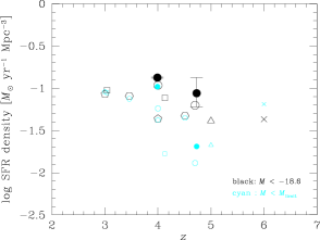
Figure 23: Cosmic star formation rate (SFR) density as a function of redshift. The black symbols indicate the SFR densities calculated by integrating the luminosity functions down to $M_{\mathrm{UV}}=-18.6$ (equivalent to $L=0.1L^{\ast}_{z=3}$ from Steidel et al. 1999), while the cyan symbols show the lower limits, i.e., the contribution from actually observed galaxies only. The filled circles represent the measurements from this study; the other points come from Steidel et al. (1999) (open squares), Iwata et al. (2003) (open triangles), Ouchi et al. (2004) (open circles), Gabasch et al. (2004) (open hexagons), Sawicki & Thompson (2006) (open pentagons), and Bouwens et al. (2005) (crosses).

5.2.2 Luminosity Dependent Evolution of the Cosmic Star Formation Rate Density
over $0\leq z\leq 6$

We examine the evolution of the cosmic SFR densities contributed from galaxies with different magnitudes over the redshift range of $0\leq z\leq 6$. Figure 24 compares their evolutionary behavior. The black, red, magenta, green, and blue symbols indicate the cosmic SFR densities from galaxies with magnitudes in the range $M<M^{\ast}_{z=3}-1.5$, $M^{\ast}_{z=3}-1.5<M<M^{\ast}_{z=3}-0.5$, $M^{\ast}_{z=3}-0.5<M<M^{\ast}_{z=3}+0.5$, $M^{\ast}_{z=3}+0.5<M<M^{\ast}_{z=3}+1.5$, and $M^{\ast}_{z=3}+1.5<M<M^{\ast}_{z=3}+2.5$, respectively. The filled circles represent our measurements, and the other symbols show the values similarly calculated using the LFs taken from the literature. There is a remarkable dependence of the evolutionary behavior of the SFR density on luminosity, as is previously noticed by Shimasaku et al. (2005) who compare the evolution of the total cosmic SFR density and the SFR density from galaxies brighter than $M=-21.3$ to find that the SFR density from bright galaxies drastically changes with time. From Figure 24, it is shown that the SFR density from fainter galaxies evolves more mildly. In addition, the peak position varies with luminosity; the contribution from fainter galaxies peaks at earlier epochs. For example, the SFR density for galaxies with $M^{\ast}_{z=3}-1.5<M<M^{\ast}_{z=3}-0.5$ rises by about an order of magnitude from $z\sim 6$ to $z\sim 4$, remains unchanged to $z\sim 3$, and then drops by more than three orders of magnitude to the present epoch, thus having a sharp peak at $z\sim 3$ – 4. On the other hand, the SFR density for galaxies with $M^{\ast}_{z=3}+1.5<M<M^{\ast}_{z=3}+2.5$ is almost constant within a factor of about two at $z\gtrsim 2$ with a blunt peak at $z\sim 4$ – 5. Iwata et al. (2003), Gabasch et al. (2004), and Sawicki & Thompson (2006) have reported different evolutions of the LBG LF from $z\sim 4$ or 5 to 3 from what we find in the SDF. At $3\lesssim z\lesssim 5$, the luminosity density of these authors shows an opposite trend that fainter galaxies evolve more rapidly. However, it is at $z\lesssim 3$ and $z\gtrsim 5$ that most drastic evolution occurs in the luminosity density. Thus, using the LFs from these authors does not qualitatively change the results on the overall evolution over $0\lesssim z\lesssim 6$ obtained here.

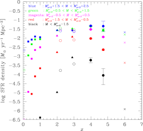
Figure 24: Cosmic star formation rate (SFR) density as a function of redshift over the redshift range of $0\leq z\leq 6$, demonstrating its luminosity dependent evolution. The black, red, magenta, green,and blue symbols indicate the SFR density from galaxies with $M<M^{\ast}_{z=3}$, $M^{\ast}_{z=3}-1.5<M<M^{\ast}_{z=3}-0.5$, $M^{\ast}_{z=3}-0.5<M<M^{\ast}_{z=3}+0.5$, $M^{\ast}_{z=3}+0.5<M<M^{\ast}_{z=3}+1.5$, and $M^{\ast}_{z=3}+1.5<M<M^{\ast}_{z=3}+2.5$, respectively. The filled circles represent the measurements from this study. The open squares comes from Wyder et al. (2005), the filled squares from Arnouts et al. (2005; GALEX), the filled triangles from Arnouts et al. (2005; HDF), the open circles from Sawicki & Thompson (2006),

and the crosses from Bouwens et al. (2005).

This luminosity-dependent evolution of the cosmic SFR density reflects the evolution of the LF discussed in §5.1. The strong increase in the SFR density for galaxies brighter than $M^{\ast}_{z=3}-0.5$ from $z\sim 6$ to $z\sim 3$ is due to the brightening of $M^{\ast}$ with time. The SFR densities for these bright galaxies then drop to the present epoch, as $M^{\ast}$ fades during the same period. The evolution of the SFR densities for galaxies fainter than $M^{\ast}_{z=3}-0.5$ is mild, since they are less sensitive to the change in $M^{\ast}$. The earlier peak position of the SFR density of fainter galaxies suggests that faint galaxies are more dominant in terms of the cosmic SFR density at earlier epochs.

We cannot completely rule out the possibility that the luminosity-dependent evolution in the cosmic SFR density seen above is not real but reflects luminosity-dependent evolution of some other properties such as dust extinction. If, for instance, galaxies have the smallest dust extinction at $z\sim 3$ – 4, then the observed $M^{\star}$ will be the brightest at these redshifts, as seen in Figure 22, even if the intrinsic, dust-corrected $M^{\star}$ does not change with redshift. In this case, the behavior of the luminosity-dependent SFR density will be qualitatively similar to that found in Figure 24. However, no observation has reported strong evolution of $E(B-V)$ at least for LBGs. The $E(B-V)$ distribution of LBGs appears to be unchanged over $z\sim 5$ and 3 (Iwata et al., 2003; Ouchi et al., 2004). In addition, $E(B-V)$ is known to be independent of apparent $M$ (Adelberger & Steidel, 2000; Ouchi et al., 2004).

5.3 Specific Star Formation Rate

We explore the evolution of what we define as the specific SFR here, i.e., the cosmic SFR per unit baryon mass in dark haloes. The specific SFR means the efficiency of star formation averaged over the all dark haloes present at a given redshift. The specific SFR is computed by dividing the cosmic SFR density, $\rho_{L}^{L>0.1L^{\ast}_{z=3}}$, by the average mass density of baryons confined in dark haloes, $\rho_{\mathrm{b}}$. Here, $\rho_{\mathrm{b}}$ is calculated by

$$\rho_{\mathrm{b}}(z) = \frac{\mathrm{\Omega}_{b}}{\mathrm{\Omega}_{m}}\int^{\infty}_{M_{\mathrm{min}}(z)}n(M,z)M\,dM,$$ (11)

where $\mathrm{\Omega}_{b}=0.05$ is the density parameter of baryons, $n(M,z)$ is the mass function of dark haloes at redshift $z$ predicted by the standard Cold Dark Matter model with $\sigma_{8}=0.9$, $M_{\mathrm{min}}(z)$ is the halo mass corresponding to a virial temperature of $1\times 10^{4}$ K. We assume here that gas does not cool (and thus stars are not formed) in dark haloes with $T<1\times 10^{4}$ K. Note that $M_{\mathrm{min}}(z)$ is much smaller than the estimated mass of haloes which host the faintest galaxies we account here, i.e., galaxies with $0.1L^{\ast}_{\mathrm{z=3}}$.

Figure 25 shows the evolution of the specific SFR over $0\leq z\leq 6$. The filled circles represent our measurements and the other symbols show the values from the literature. The dotted line in the figure shows $(1+z)^{3}$ evolution. We find that the specific SFR increases in proportion to $(1+z)^{3}$ up to $z\sim 4$. In other words, the star formation efficiency in the universe rises with redshift. At $z\gtrsim 4$, on the other hand, the specific SFR appears to decrease.

Figure 25: Specific star formation rate (SFR) versus $(1+z)$ over $0\leq z\leq 6$. Symbols are the same as in Figure 24. The dotted line shows evolution in power-law, specific $\mathrm{SFR}\propto(1+z)^{3}$.

Here, according to the standard Cold Dark Matter model, the average internal density in physical units of baryons in dark haloes virialized at a given redshift, $\left<\rho_{\mathrm{b}}^{\mathrm{DH}}\right>$, is known to be approximately proportional to the average mass density of the universe at that time, and the average mass density of the universe changes as $(1+z)^{3}$. Therefore, it implies that the specific SFR increases approximately in proportion to $\left<\rho_{\mathrm{b}}^{\mathrm{DH}}\right>$ up to $z\sim 4$. To put it another way, since the specific SFR is the internal density of SFR in dark haloes, $\left<\rho_{\mathrm{SFR}}^{\mathrm{DH}}\right>$, divided by $\left<\rho_{\mathrm{b}}^{\mathrm{DH}}\right>$, this result can be expressed in terms of $\left<\rho_{\mathrm{SFR}}^{\mathrm{DH}}\right>$ and $\left<\rho_{\mathrm{b}}^{\mathrm{DH}}\right>$ as:

$$\left<\rho_{\mathrm{SFR}}^{\mathrm{DH}}\right> \propto \left<\rho_{\mathrm{b}}^{\mathrm{DH}}\right>^{2}.$$ (12)

It is surprising that the star formation in galaxies obeys such a simple power law over $90\%$ of the cosmic history ($0<z\lesssim 4$). Equation (12) resembles the Schmidt law (Schmidt, 1959) of nearby disk galaxies, a relationship between the disk-averaged SFR and cold gas surface densities of $\Sigma_{\mathrm{SFR}}=\mathrm{const.}\times\Sigma_{\mathrm{gas}}^{N}$ with $N\sim 1.4$ (Kennicutt 1998).

We present here one possible explanation of the observed behavior of the specific SFR. The analytical modeling of galaxy formation based on the CDM model by Hernquist & Springel (2003) shows that the gas cooling rate, $\dot{M}_{\mathrm{cool}}/M_{\mathrm{DH}}$, of dark haloes roughly scales with $H(z)^{2}$, or equivalently with $(1+z)^{3}$ as $H(z)$ is approximately proportional to $(1+z)^{3/2}$ in our cosmology. They also find that the star formation rate in dark haloes scales with the cooling rate at low and intermediate redshifts, while it becomes to be no longer dependent on the cooling rate at redshifts larger than a certain limit, where the internal density of haloes is so high that the cooling time is shorter than the consumption rate of cooled gas into stars. If we adopt this modeling, then our result implies that the cosmic SFR is primarily determined by the gas cooling rate at $z\lesssim 4$, while it is governed by the conversion rate of cooled gas into stars at larger redshifts.

Of course, the cooling rate may not be the major factor determining the cosmic star formation rate. There are many other factors on which the star formation in galaxies can largely depends, such as the feedback by galactic winds, the UV background radiation field, and environmental effects like galaxy merging and interactions. Since the relative importance of these factors will vary with the mass of dark haloes, it will be interesting to measure the specific SFR as a function of halo mass.

6 SUMMARY AND CONCLUSIONS

We investigated the luminosity functions and star formation rates of Lyman-break galaxies (LBGs) at $z\sim 4$ and 5 based on the optical imaging data obtained in the Subaru Deep Field (SDF) Project. The SDF Project is a program conducted by Subaru Observatory to carry out a deep and wide galaxy survey in the SDF.

Three samples of LBGs in a contiguous 875 arcmin² area are constructed. One consists of LBGs at $z\sim 4$ selected with the $B\!-\!R$ vs $R\!-\!i^{\prime}$ diagram ($BRi^{\prime}$-LBGs). The other two consist of LBGs at $z\sim 5$ selected with two kinds of two-color diagrams: $V\!-\!i^{\prime}$ vs $i^{\prime}\!-\!z^{\prime}$ ($Vi^{\prime}z^{\prime}$-LBGs) and $R\!-\!i^{\prime}$ vs $i^{\prime}\!-\!z^{\prime}$ ($Ri^{\prime}z^{\prime}$-LBGs). The number of LBGs detected is $3,808$ for $BRi^{\prime}$-LBGs, 539 for $Vi^{\prime}z^{\prime}$-LBGs, and 240 for $Ri^{\prime}z^{\prime}$-LBGs. The adopted selection criteria are proved to be fairly reliable by the spectroscopic data. We use Monte Carlo simulations to estimate the completeness and the fraction of contamination by interlopers. The redshift distribution functions obtained by the simulations are well consistent with the redshift distributions of spectroscopically identified objects in the LBG samples.

We derived the luminosity functions at rest-frame ultraviolet wavelengths down to as faint as $M_{\mathrm{UV}}=-19.2$ at $z\sim 4$ and $M_{\mathrm{UV}}=-20.3$ at $z\sim 5$. The cosmic star formation rate (SFR) density was measured from the ultraviolet luminosity density derived by integrating the luminosity functions. On the basis of the observed SFR density and the standard Cold Dark Matter model, the cosmic SFR per unit baryon mass in dark haloes, i.e., the specific SFR, is computed. Combining the results obtained in this work with those taken from the literature, we reached the following conclusions:

1. Clear evolution of the luminosity function is detected. The characteristic magnitude $M^{\ast}$ changes strongly over the redshift range of $0\leq z\leq 6$. It brightens by about 1 mag from $z\sim 6$ to $z\sim 4$, remains unchanged to $z\sim 3$ and then fades by about 3 mag from $z\sim 3$ to $z\sim 0$. On the other hand, the normalization factor, $\phi^{\ast}$, and the faint-end slope, $\alpha$, are almost constant over $0.5\lesssim z\lesssim 6$.

2. The measurements of the SFR density at $z\sim 4$ and $z\sim 5$ are greatly improved, since the luminosity functions are derived down to very faint magnitudes. Hence, the evolutionary behavior of the SFR density is more constrained. The cosmic SFR density does not drop from $z\sim 3$ to $z\sim 4$, and the decrease from $z\sim 4$ to $z\sim 5$, if any, cannot be larger than a factor of about five.

3. The SFR density contributed from brighter galaxies changes more drastically with cosmic time. The contribution from galaxies brighter than $M^{\ast}_{z=3}-0.5$ has a sharp peak around $z=3$ – 4, while that from galaxies fainter than $M^{\ast}_{z=3}-0.5$ evolves relatively mildly with a broad peak at earlier epoch. This luminosity-dependent evolution of the cosmic SFR density suggests that the galaxy population that contributes to the total SFR density in the universe varies with time, reflecting the evolution of the luminosity function.

4. The specific SFR is found to scale with redshift as $(1+z)^{3}$ up to $z\sim 4$, implying that the efficiency of star formation is on average higher at higher redshift in proportion to the cooling rate within dark haloes. It seems that this is not simply the case at $z\gtrsim 4$.

References

- Adelberger & Steidel (2000) Adelberger, K. L. & Steidel, C. C. 2000, ApJ, 544, 218
- Arnouts et al. (2005) Arnouts, S., et al. 2005, ApJ, 619, L43
- Bertin & Arnouts (1996) Bertin, E. & Arnouts, S. 1996, A&AS, 117, 393
- Bouwens et al. (2004) Bouwens, R. J., et al. 2004, ApJ, 616, L79
- Bouwens et al. (2005) Bouwens, R. J., Illingworth, G. D., Blakeslee, J. P., & Franx, M. 2005, ApJ, in press (astro-ph/0509641)
- Bunker et al. (2004) Bunker, A. J., Stanway, E. R., Ellis, R. S., & McMahon, R. G. 2004, MNRAS, 355, 374
- Calzetti et al. (2000) Calzetti, D., Armus, L., Bohlin, R. C., Kinney, A. L., Koornneef, J., & Storchi-Bergmann, T. 2000, ApJ, 533, 682
- Capak et al. (2004) Capak, P., et al. 2004, AJ, 127, 180
- Chapman et al. (2005) Chapman, S. C., Blain, A. W., Smail, I., & Ivison, R. J. 2005, ApJ, 622, 772
- Dickinson et al. (2004) Dickinson, M., et al. 2004, ApJ, 600, L99
- Faber et al. (2003) Faber, S. M., et al. 2003, Proc. SPIE, 4841, 1657
- Franx et al. (2003) Franx, M., et al. 2003, ApJ, 587, L79
- Furusawa et al. (2000) Furusawa, H., Shimasaku, K., Doi, M., & Okamura, S. 2000, ApJ, 534, 624
- Gabasch et al. (2004) Gabasch, A., et al. 2004, A&A, 421, 41
- Guhathakurta et al. (1990) Guhathakurta, P., Tyson, J. A., & Majewski, S. R. 1990, ApJ, 357, L9
- Gunn & Stryker (1983) Gunn, J. E. & Stryker, L. L. 1983, ApJS, 52, 121
- Hernquist & Springel (2003) Hernquist, L. & Springel, V. 2003, MNRAS, 341, 1253
- Hopkins (2004) Hopkins, A. M. 2004, ApJ, 615, 209
- Iwata et al. (2003) Iwata, I., Ohta, K., Tamura, N., Ando, M., Wada, S., Watanabe, C., Akiyama, M., & Aoki, K. 2003, PASJ, 55, 415
- Iye et al. (2004) Iye, M., et al. 2004, PASJ, 56, 381
- Kashikawa et al. (2002) Kashikawa, N., et al. 2002, PASJ, 54, 819
- Kashikawa et al. (2003) Kashikawa, N., et al. 2003, AJ, 125, 53
- Kashikawa et al. (2004) Kashikawa, N., et al. 2004, PASJ, 56, 1011
- Kashikawa et al. (2006) Kashikawa, N., et al. 2006, ApJ, in press (astro-ph/0509564)
- Kennicutt (1998) Kennicutt, R. C., Jr. 1998, ARA&A, 36, 189
- Kodama & Arimoto (1997) Kodama, T. & Arimoto, N. 1997, A&A, 320, 41
- Le Fèvre et al. (2005) Le Fèvre, O., et al. 2005, Nature, 437, 519
- Lehnert & Bremer (2003) Lehnert, M. D. & Bremer, M. 2003, ApJ, 593, 630
- Madau (1995) Madau, P. 1995, ApJ, 441, 18
- Maihara et al. (2001) Maihara, T., et al. 2001, PASJ, 53, 25
- Meiksin (2006) Meiksin, A. 2006, MNRAS, 365, 807
- Nagashima et al. (2005) Nagashima, M., Yahagi, H., Enoki, M., Yoshii, Y., & Gouda, N. 2005, ApJ, in press (astro-ph/0508085)
- Miyazaki et al. (2002) Miyazaki, S., et al. 2002, PASJ, 54, 833
- Oke & Gunn (1983) Oke, J. B. & Gunn, J. E. 1983, ApJ, 266, 713
- Ouchi (2003) Ouchi, M. 2003, Ph.D. Thesis, The University of Tokyo
- Ouchi et al. (2004) Ouchi, M., et al. 2004, ApJ, 611, 660
- Papovich et al. (2001) Papovich, C., Dickinson, M., & Ferguson, H. C. 2001, ApJ, 559, 620
- Sawicki & Thompson (2006) Sawicki, M. & Thompson, D. 2006, ApJ, 642, 653
- Shimasaku et al. (2005) Shimasaku, K., Ouchi, M., Furusawa, H., Yoshida, M., Kashikawa, N., & Okamura, S. 2005, PASJ, 57, 447
- Schechter (1976) Schechter, P. 1976, ApJ, 203, 297
- Schlegel et al. (1998) Schlegel, D. J., Finkbeiner, D. P., & Davis, M. 1998, ApJ, 500, 525
- Schmidt (1959) Schmidt, M. 1959, ApJ, 129, 243
- Smail, Ivison, & Blain (1997) Smail, I., Ivison, R. J., & Blain, A. W. 1997, ApJ, 490, L5
- Spergel et al. (2003) Spergel, D. N., et al. 2003, ApJS, 148, 175
- Stanway et al. (2003) Stanway, E. R., Bunker A. J., & McMahon, R. G. 2003, MNRAS, 342, 439
- Steidel & Hamilton (1992) Steidel, C. C. & Hamilton, D. 1992, AJ, 104, 941
- Steidel et al. (1999) Steidel, C. C., Adelberger, K. L., Giavalisco, M., Dickinson, M., & Pettini, M. 1999, ApJ, 519, 1
- Steidel et al. (2003) Steidel, C. C., Adelberger, K. L., Shapley, A. E., Pettini, M., Dickinson, M., & Giavalisco, M. 2003, 592, 728
- Wyder et al. (2005) Wyder, T. K., et al. 2005, ApJ, 619, L15
- Yagi et al. (2002) Yagi, M., Kashikawa, N., Sekiguchi, M., Doi, M., Yasuda, N., Shimasaku, K., & Okamura, S. 2002, AJ, 123, 66
- Yan et al. (2003) Yan, H., Windhorst, R. A., & Cohen, S. H. 2003, ApJ, 585, L93