Using Weak Lensing Dilution to Improve Measurements of the Luminous and Dark Matter in A1689

Elinor Medezinski¹¹affiliation: School of Physics and Astronomy, Tel Aviv University, Israel , Tom Broadhurst¹¹affiliation: School of Physics and Astronomy, Tel Aviv University, Israel , Keiichi Umetsu²²affiliation: Institute of Astronomy and Astrophysics, Academia Sinica, P. O. Box 23-141, Taipei 106, Taiwan, Repucblic of China , Dan Coe ³³affiliation: Physics and Astronomy Dept, Johns Hopkins University, Baltimore Maryland, USA ⁴⁴affiliation: Instituto de Astrofísica de Andalucía (CSIC), Granada, Spain , Narciso Benítez⁴⁴affiliation: Instituto de Astrofísica de Andalucía (CSIC), Granada, Spain , Holland Ford³³affiliation: Physics and Astronomy Dept, Johns Hopkins University, Baltimore Maryland, USA , Yoel Rephaeli ¹¹affiliation: School of Physics and Astronomy, Tel Aviv University, Israel , Nobuo Arimoto⁵⁵affiliation: National Astronomical Observatory of Japan, Mitaka 181-8588, Japan , Xu Kong⁶⁶affiliation: Center for Astrophysics, University of Science and Technology of China, Hefei, 230026, Anhui, PR China

Abstract

The E/SO sequence of a cluster defines a boundary redward of which a reliable weak lensing signal can be obtained from background galaxies, uncontaminated by cluster members. For bluer colors, both background and cluster galaxies are present, reducing the average distortion signal by the proportion of unlensed cluster members. In deep Subaru and HST/ACS images of A1689, we show that the tangential distortion of galaxies with bluer colors falls rapidly toward the cluster center relative to the background reference level provided by the red background. We use this dilution effect to derive the cluster light profile and luminosity function to large radius, with the advantage that no subtraction of far-field background counts is required. The light profile of A1689 is found to decline steadily to the limit of the data, $r<2~{}h^{-1}$ Mpc, with a constant slope, $d\log(L)/d\log(r)=-1.12\pm 0.06$ , unlike the lensing mass profile which steepens continuously with radius, so that $M/L$ peaks at an intermediate radius, $\simeq 100~{}h^{-1}$ kpc. A flatter behaviour is found for the more physically meaningful ratio of dark-matter to stellar-matter, when account is made of the color-mass relation of cluster members. We derive a cluster luminosity function with a flat faint-end slope of $\alpha=-1.05\pm 0.07$ , nearly independent of radius and with no faint upturn to $M_{i^{\prime}}<{-12}$ . We establish that the very bluest objects are negligibly contaminated by the cluster ( $[V-i^{\prime}]_{AB}<0.2$ ), because their distortion profile rises continuously towards the center following the red background ( $[V-i^{\prime}]_{AB}>1.2$ ), but is offset higher by $\simeq 20\%$ . This larger amplitude is consistent with the greater estimated depth of the faint blue galaxies $\langle z\rangle\sim 2$ compared to $\langle z\rangle\sim 0.85$ for the red background, a purely geometric effect. With a larger sample of background galaxies behind several clusters we may use this geometric effect to constrain the cosmological parameters in a model independent way, by comparing the weak lensing strength over a wide range of photometrically derived redshifts. Finally, we improve upon our earlier modeling of the mass profile by combining both the red and blue background populations, and very clearly exclude low concentration profiles predicted for massive CDM dominated haloes.

Subject headings:

cosmology: observations – gravitational lensing – galaxies: clusters: individual(Abell 1689) – galaxies: luminosity function

1. Introduction

The influence of “Dark matter” is strikingly evident in the centers of massive galaxy clusters, where large velocity dispersions are measured and giant arcs are often visible. Cluster masses may be estimated by several means, leading to exceptionally high central mass-to-light ratios, $M/L_{R}\sim 100-300h(M/L_{R})_{\odot}$ (Carlberg et al., 2001), far exceeding both the mass of stars comprising the light of the cluster galaxies and the mass of plasma derived from X-ray emission and the SZ effect. Reasonable consistency is claimed between dynamical, hydrodynamical and lensing-based estimates of cluster masses, supporting the conventional understanding of gravity. However, the high mass-to-light ratio requires that an unconventional non-baryonic dark material dominates the mass of clusters, whose origin remains very unclear.

In detail, discrepancies are often reported between masses derived from strong lensing and X-ray measurements, with the claimed X-ray masses often lower in the centers of clusters. High resolution X-ray emission and temperature maps reveal that the majority of local clusters undergo repeated merging with sub-clumps, and obvious shock fronts are seen in some cases (Markevitch et al., 2002; Reiprich et al., 2004). The double cluster 1E 0657–56 (a.k.a., the “bullet” cluster, $z=0.296$ ) is the most extreme example studied, where the associated gas forms a flattened luminous shock-heated structure lying between the two large distinct clusters, clearly indicating these two bodies collided recently at a high relative velocity (Markevitch et al., 2004), with the gas remaining in between while the cluster galaxies have passed through each other relatively collisionlessly. Very interestingly, the weak lensing signal follows the double structure of the clusters, rather than the gas in between, cleanly demonstrating that the bulk of the matter is collisionless and dark (Clowe et al., 2004). This system favors the standard cold dark matter (CDM) scenario, places a restrictive limit on the interaction cross-section of any fermionic dark matter, and disfavors a class of alternative gravity theories in which only baryons are present (Clowe et al., 2004). Smaller but significant discrepancies of the same sort are also claimed for other interacting clusters (Natarajan et al., 2002; Jee et al., 2005).

Many clusters show no apparent signs of significant ongoing interaction; these have centrally symmetric X-ray emission and little obvious substructure (Allen, 1998), and for some of these the lensing and X-ray (or dynamical) derived masses are claimed to agree, as would be expected for relaxed systems (e.g., Arabadjis et al., 2002; Rines et al., 2003; Diaferio et al., 2005). More generally, since the dyanmics of dark matter and most cluster galaxies is essentially collisionless, we would expect them to have similar radial profiles. Biasing inherent in hierarchical growth may significantly modify this similarity (Kauffmann et al., 1997), and dynamical friction is expected to concentrate the relatively more massive galaxies in the core. These together with tidal effects may help to account for the unique properties of cD galaxies. Hence comparisons of the mass profile with the light profile of the cluster galaxies are expected to provide an additional insight into the formation of clusters and the nature of dark matter.

Recent improvements in the quality of data useful for weak and strong lensing studies now allow the construction of much more definitive mass profiles that are sufficiently precise to test the predictions of popular models, relatively free of major assumptions. The inner mass profiles of several clusters have been constrained in some detail via lensing, using multiply lensed background galaxies (Kneib et al., 1996; Hammer et al., 1997; Sand et al., 2002; Gavazzi et al., 2003; Sand et al., 2004; Broadhurst et al., 2005a; Sharon et al., 2005). The statistical effects of weak lensing have been used to extend the mass profile to larger radii. The mass profiles derived from these observations have been claimed to show NFW-like behaviour (Navarro, Frenk, & White, 1997), with a continuous flattening towards the center, but with higher density concentrations than expected. This is particularly evident for A1689, for which we have constructed the highest quality lensing based mass profile to date, combining over 100 multiply-lensed images and weak lensing effects of distortion and magnification from Subaru (Broadhurst et al., 2005a, b).

A lesson learned from this earlier work is the importance of carefully selecting a background population to avoid contamination by the lensing cluster. It is not enough to simply exclude a narrow band containing the obvious E/SO sequence, following common practice, because the lensing signal of the remainder is found to fall rapidly towards the cluster center, in contrast to the uncontaminated population of background galaxies lying redward of the cluster sequence (Broadhurst et al., 2005b). In the well studied case of A1689, there has been a long standing discrepancy between the strong and weak lensing effects, with the weak lensing signal underpredicting the observed Einstein radius by a factor of $\sim 2.5$ (Clowe & Schneider, 2001; Bardeau et al., 2005), based only on a minimal rejection of obvious cluster members using one or two-band photometry.

In our recent weak lensing analysis of Subaru images of A1689 the above behaviour was found when we rejected only the cluster sequence in the same way as others. This resulted in a relatively shallow trend of the weak lensing signal with radius and consequently an underprediction of the Einstein radius accounting for the earlier discrepancy (Broadhurst et al., 2005b) . If, however, one selects only objects redder than the cluster sequence for the lensing analysis, then the weak tangential distortion continues to rise all the way to the Einstein radius in very good agreement with the strong lensing strength. This red population is naturally expected to comprise only background galaxies, made redder by relatively large k-corrections and with negligible contamination by cluster members, since the bulk of the reddest cluster members are the early-type galaxies defined by the cluster sequence. However, for galaxies with colors bluer than the cluster sequence, cluster members will be present along with background galaxies since the cluster population extends to bluer colors of the later-type members, overlapping in color with the blue background. The effect of the cluster members is simply to reduce the strength of the weak lensing signal when averaged over a statistical sample, in proportion to the fraction of cluster members whose orientations are randomly distributed, therefore diluting the lensing signal relative to the reference background level derived from the red background population.

We can turn this dilution effect to our advantage and use it to derive properties of the cluster population, in particular the radial light profile, for comparison with the dark matter profile. Deriving a light profile this way has advantages over the usual approach to defining cluster membership. The inherent fluctuations in the number counts of the background population are a significant source of uncertainty in the usual approach of subtracting the far-field level when defining the cluster population (e.g., Paolillo et al., 2001; Andreon et al., 2005; Pracy et al., 2005). This uncertainty is often cited as a potential explanation for the substantial variation reported between luminosity functions derived for different clusters, particularly in the outskirts of clusters, where not only is the density of galaxies lower, but their colors are bluer, thus harder to distinguish from the background using photometry alone.

In § 2 we describe the observations and photometry of the Subaru images of A1689. In § 3 we describe the distortion analysis applied to the Subaru data. The distortion analysis of ACS images of A1689 is described in § 4. In § 5 we describe the photometric redshift analysis of the Subaru and ACS images with reference to the Capak et al. (2004) sample of deep multi-color Subaru images. Our weak lensing dilution analysis of the Subaru images is described in § 6. In § 7 we go on to derive the cluster luminosity profile and color, and in § 8 the cluster luminosity function is deduced at several radial positions. In § 9 we determine the $M/L$ profile, and in § 10 we do a consistency check for the mass derived in this paper with previous estimations. Our conclusions are summarized in § 11.

The concordance $\Lambda$ CDM cosmology is adopted ( $\Omega_{M}=0.3$ , $\Omega_{\Lambda}=0.7$ but $h$ is left in units of $H_{0}/100$ km s^-1 Mpc^-1, for easier comparison with earlier work).

2. Subaru Imaging reduction and Sample selection

We have retrieved Suprime-Cam imaging of A1689 in $V$ (1920s) and SDSS $i^{\prime}$ (2640s) from the Subaru archive, SMOKA. ¹¹1http://smoka.nao.ac.jp. Reduction software developed by Yagi et al. (2002) is used for flat-fielding, instrumental distortion correction, differential refraction, PSF matching, sky subtraction, and stacking. The resulting FWHM is 0″.82 in $V$ and 0″.88 in $i^{\prime}$ with 0″.202 pix^-1, covering a field of $30^{\prime}\times 25^{\prime}$ .

Refer to caption — Figure 1.— Color vs. magnitude diagram for A1689 cluster galaxies. The E/SO sequence is apparent at $(V-i^{\prime})\sim 0.8$ where there is an overdensity of bright galaxies. The red points represent the background sample of galaxies redder than the E/SO sequence. The blue points represent a background sample of the bluest objects in the field. The green points cover a range of color chosen to include the cluster sequence and bluer cluster members, but in addition background galaxies are also present whose colors fall in this range.

Table 1Sample Selection

Sample Name	mag limit	color limit	N	n [ $h^{2}$ Mpc^-2]	$<z>$	$<D>$
red	$18<i^{\prime}<26.5$	$0.2<(V-i^{\prime})-(V-i^{\prime})_{E/SO}<2.5$	11774	966.1	0.871 $\pm$ 0.045	0.693 $\pm$ 0.012
green	$16<i^{\prime}<26.5$	$-0.3<(V-i^{\prime})-(V-i^{\prime})_{E/SO}<0.1$	11963	981.6	1.429 $\pm$ 0.093	0.728 $\pm$ 0.015
blue	$23<i^{\prime}<26.5$	$-1.2<(V-i^{\prime})-(V-i^{\prime})_{E/SO}<-0.45$	2459	201.8	2.012 $\pm$ 0.124	0.830 $\pm$ 0.011

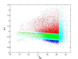
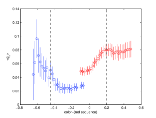
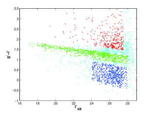
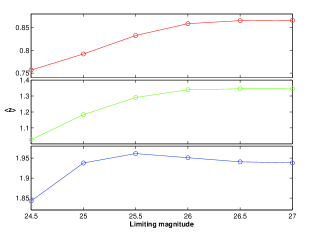
Photometry is based on a combined $V+i^{\prime}$ image using SExtractor (Bertin & Arnouts, 1996). The limiting magnitudes are $V=26.5$ and $i^{\prime}=25.9$ for a $3\sigma$ detection within a $2$ ″aperture. We define three galaxy samples according to color and magnitude – “red”, “green”, and “blue” (see table 1 for summary), and for all our samples we define a limiting magnitude of $i^{\prime}<26.5$ , to avoid incompleteness, as shown in Figure 1. The red galaxy sample consists of galaxies $0^{m}.2$ redder than the E/SO sequence of the cluster, which is accurately defined by the linear relation $(V-i^{\prime})_{E/SO}=-0.03525i^{\prime}+1.505$ , and up to $2^{m}.5$ redder than this line to include the majority of the background red population. Very red dropout galaxies may be detected beyond this point. Indeed, one spectroscopically confirmed example at $z=4.82$ has been detected behind this cluster (Frye et al., 2002), and such cases are excluded by this upper limit, so that we do not need to make an uncertain correction for the level of their weak lensing signal which will be significantly larger than for the bulk of the background red galaxy population. As we will show in § 5, most of these red background galaxies are at a much lower mean redshift of $\langle z\rangle\sim 0.85$ . The red galaxy sample is redder than the cluster sequence, made so by relatively large k-corrections, being largely comprised of early to mid-type galaxies at moderate redshift (see § 5). Cluster members are not expected to extend to these colors in any significant numbers because the intrinsically reddest class of cluster galaxies, E/SO galaxies, are defined by the cluster sequence and lie comfortably blueward of the chosen sample limit (see Fig. 1), so that even large photometric errors will not carry them into the red sample. This can be demonstrated readily, as shown in Figure 2, where we plot the mean lensing strength as a function of color by moving the lower color limit progressively blueward, finding a sharp drop in the lensing signal at our limit, $(V-i^{\prime})<(V-i^{\prime})_{E/SO}+0.2$ , when the cluster sequence starts to contribute significantly, thereby reducing the mean lensing signal.

We define the blue galaxy sample as objects $0^{m}.45$ bluer than the sequence line, with the magnitude limit in the interval $23<i^{\prime}<26.5$ , so as to take only the very faint blue galaxies which - as we establish below - are also negligibly contaminated by the cluster, with a weak lensing signal which has the same radial dependence as the red galaxy sample. We have explored the definition of the blue sample when we realized that the bluest objects in the field have a continuously rising weak lensing signal towards the cluster center like the red galaxies, so that the “contamination” is minimal with an insignificant effect on the quantities of interest for our purposes. Figure 2 shows that as the blue sample upper color limit is advanced redwards, the integrated strength of the mean weak lensing signal declines markedly within $0^{m}.45$ of the cluster sequence, at $(V-i^{\prime})>(V-i^{\prime})_{E/SO}-0.45$ . The reduction in signal is more gradual than for the red population (both illustrated in Fig. 2) because the blue cluster members do not lie along a sharp sequence but contribute a diminishing fraction relative to the background at bluer colors.

The green galaxy sample is simply selected to lie between the red and blue samples defined above, ${(V-i^{\prime})_{E/SO}}^{+0.1}_{-0.3}$ (Fig. 1), with generous limits set to include the vast majority of cluster galaxies, since - as we have established - both the red and blue samples are negligibly contaminated by cluster members, and hence the vast majority of cluster members must lie within this intermediate range of color. A narrow gap on each side of these samples is left out of our analysis to ensure that the definition of the background does not encrouch on the cluster population. Note that unlike the green sample containing the cluster population, the background populations do not need to be complete in any sense but should simply be well defined and contain only background. Increasing the green sample to cover these narrow gaps does not lead to any particularly significant change in our conclusions, but only increases somewhat the level of noise by including relatively more background galaxies. Within the green sample there are of course background galaxies, and the purpose of this paper is to make use of the relative proportion of these cluster and background populations via weak lensing to establish the properties of the cluster galaxy population, by using the the dilution of the weak lensing signal of the background galaxies due to the cluster members.

3. Distortion Analysis of Subaru Images

We use the IMCAT package developed by N. Kaiser ²²2http://www.ifa.hawaii/kaiser/IMCAT to perform object detection, photometry and shape measurements, following the formalism outlined in (Kaiser, Squires, & Broadhurst, 1995, hereafter KSB). We have modified the method somewhat following the procedures described in Erben et al. (2001, see Section 5).

To obtain an estimate of the reduced shear, $g_{\alpha}=\gamma_{\alpha}/(1-\kappa)$ , we measure the image ellipticity $e_{\alpha}$ from the weighted quadrupole moments of the surface brightness of individual galaxies. Firstly the PSF anisotropy needs to be corrected using the star images as references:

e^{\prime}_{\alpha}=e_{\alpha}-P_{sm}^{\alpha\beta}q^{*}_{\beta}

(1)

where $P_{sm}$ is the smear polarizability tensor being close to diagonal, and $q^{*}_{\alpha}=(P_{*sm})^{-1}_{\alpha\beta}e_{*}^{\beta}$ is the stellar anisotropy kernel. We select bright, unsaturated foreground stars identified in a branch of the half-light radius ( $r_{h}$ ) vs. magnitude ( $i^{\prime}$ ) diagram ( $20<i^{\prime}<22.5$ , $\left<r_{h}\right>_{\rm median}=2.38$ pixels) to calculate $q^{*}_{\alpha}$ . In order to obtain a smooth map of $q^{*}_{\alpha}$ which is used in equation (1), we divided the $9{\rm K}\times 7.4{\rm K}$ image into $5\times 4$ chunks each with $1.8{\rm K}\times 1.85{\rm K}$ pixels, and then fitted the $q^{*}$ in each chunk independently with second-order bi-polynomials, $q_{*}^{\alpha}(\vec{\theta})$ , in conjunction with iterative $\sigma$ -clipping rejection on each component of the residual $e^{*}_{\alpha}-P_{*sm}^{\alpha\beta}q^{*}_{\beta}(\vec{\theta})$ . The final stellar sample consists of 540 stars, or the mean surface number density of $n_{*}=0.72$ arcmin^-2. From the rest of the object catalog, we select objects with $2.4\lesssim r_{h}\lesssim 15$ pixels as an $i^{\prime}$ -selected weak lensing galaxy sample, which contains $61,115$ galaxies or $\bar{n}_{g}\simeq 81$ arcmin^-2. It is worth noting that the mean stellar ellipticity before correction is $(\bar{e_{1}}^{*},\bar{e_{2}}^{*})\simeq(-0.013,-0.018)$ over the data field, while the residual $e^{*}_{\alpha}$ after correction is reduced to ${\bar{e}^{*{\rm res}}_{1}}=(0.47\pm 1.32)\times 10^{-4}$ , ${\bar{e}^{*{\rm res}}_{2}}=(0.54\pm 0.94)\times 10^{-4}$ . The mean offset from the null expectation is $|\bar{e}^{*\rm res}|=(0.71\pm 1.12)\times 10^{-4}$ . On the other hand, the rms value of stellar ellipticities, $\sigma_{e*}\equiv\left<|e^{*}|^{2}\right>$ , is reduced from $2.64\%$ to $0.38\%$ when applying the anisotropic PSF correction.

Second, we need to correct the isotropic smearing effect on image ellipticities caused by seeing and the window function used for the shape measurements. The pre-seeing reduced shear $g_{\alpha}$ can be estimated from

g_{\alpha}=(P_{g}^{-1})_{\alpha\beta}e^{\prime}_{\beta}

(2)

with the pre-seeing shear polarizability tensor $P^{g}_{\alpha\beta}$ . We follow the procedure described in Erben et al. (2001) to measure $P^{g}$ (see also § 3.4 of Hetterscheidt et al., 2006). We adopt the scalar correction scheme, namely,

P^{g}_{\alpha\beta}=\frac{1}{2}{\rm tr}[P^{g}]\delta_{\alpha\beta}\equiv P^{g}_{\rm s}\delta_{\alpha\beta}

(3)

(Hudson et al., 1998; Hoekstra et al., 1998; Erben et al., 2001; Hetterscheidt et al., 2006). The $P_{g}^{\rm s}$ measured for individual objects are still noisy especially for small and faint objects. We thus adopt a smoothing scheme in object parameter space proposed by Van Waerbeke et al. (2000, see also , ). We first identify thirty neighbors for each object in $r_{g}$ - $i^{\prime}$ parameter space. We then calculate over the local ensemble the median value $\langle P_{g}^{\rm s}\rangle$ of $P_{g}^{\rm s}$ and the variance $\sigma^{2}_{g}$ of $g=g_{1}+ig_{2}$ using equation (2). The dispersion $\sigma_{g}$ is used as an rms error of the shear estimate for individual galaxies. The mean variance $\bar{\sigma}_{g}^{2}$ over the sample is obtained as $\simeq 0.171$ , or $\sqrt{\bar{\sigma}_{g}^{2}}\approx 0.41$ .

In the previous study by Broadhurst et al. (2005b), those objects that yield a negative value of the raw $P_{g}^{\rm s}$ estimate were removed from the final galaxy catalog to avoid noisy shear estimates. On the other hand, in the present study, we use all of the galaxies in our weak lensing sample including galaxies with $P_{g}^{\rm s}<0$ . After smoothing $P_{g}^{\rm s}$ in the object parameter space, all of the objects yield positive values of $\left<P_{g}^{\rm s}\right>$ , with the minimum of $\approx 0.04$ . The median value of $\left<P_{g}^{\rm s}\right>$ over the weak lensing galaxy sample, including galaxies with $P_{g}^{\rm s}<0$ , is calculated as $\approx 0.32$ . For a reference, the sub-sample of galaxies with $P_{g}^{\rm s}>0$ gives the median average of $\approx 0.33$ , mostly weighted by galaxies with $r_{g}=2-2.5$ pixels. Finally, we use the following estimator for the reduced shear:

g_{\alpha}=e^{\prime}_{\alpha}/\left<P_{g}^{\rm s}\right>.

(4)

The quadratic shape distortion of an object is described by the complex reduced-shear, $g=g_{1}+ig_{2}$ . The tangential component $g_{T}$ is used to obtain the azimuthally averaged distortion due to lensing, and computed from the distortion coefficients $g_{1},g_{2}$ :

g_{T}=-(g_{1}\cos 2\theta+g_{2}\sin 2\theta),

(5)

where $\theta$ is the position angle of an object with respect to the cluster center, and the uncertainty in the $g_{T}$ measurement is $\sigma\equiv\sigma_{g}/\sqrt{2}$ in terms of the rms error $\sigma_{g}$ for the complex shear measurement. The cluster center is well determined from symmetry of the strong lensing pattern (Broadhurst et al., 2005a). The estimation of $g_{T}$ only has significance when evaluated statistically over large number of galaxies, since galaxies themselves are not round objects but have a wide spread in intrinsic shapes and orientations. In radial bins we calculate the weighted average of the $g_{T}$ s and the weighted error:

	$\displaystyle\langle{}g_{T}(r_{n})\rangle{}$	$\displaystyle=$	$\displaystyle\frac{\sum{}g_{T}/\sigma^{2}}{\sum{}1/\sigma^{2}}$		(6)
	$\displaystyle\sigma_{T}(r_{n})$	$\displaystyle=$	$\displaystyle\left(\sum 1/\sigma^{2}\right)^{-1/2}.$		(7)

It has been shown that such weights depend on the size of the objects but mostly on their magnitudes (see e.g. Hoekstra et al. (2006)). Therefore, as apparent magnitude increases with redshift the redshift distribution of sources will be modified to some extent by this weighting scheme. We have investigated this using the catalogue of Capak et al. (2004) as here photometric redshifts are estimated (see § 5 for a fuller desrciption of the photometric properties of this sample). First, we generated from the Capak catalog blue/red background galaxy samples with the same color-magnitude criteria as the present study. We then derived an i’-magnitude vs. photo-z relation for each galaxy sub-sample. We subdivided the data into magnitude (i’) bins and derived a magnitude (i’) vs. photo-z relation using median averaging.

We then assume this magnitude-redshift relation holds in our A1689 data and obtain for each galaxy in A1689 an estimate of redshift via the magnitude – photo-z relation. It is then straightforward to have an effective redshift distribution taking into account weak lensing statistical weights, w. We can see a qualitative feature that although low-z background galaxies are more strongly weighted than higher-z ones, the effect on our observed redshift distribution is negligible because our redshift selection window does not sample these larger angle, lower redshift objects, but rather the more distant faint population whose small anglular sizes are heavily influenced by the seeing.

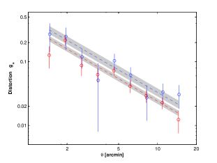
In Figure 3 we compare the radial profile of $g_{T}$ of the red and blue samples defined above. These have a very similar form implying that the blue sample, like the red sample, is dominated by background galaxies with negligible dilution by cluster members even at small radius where the cluster overdensity is large. Very interestingly a clear offset is visible between these profiles over the full range of radius, with the amplitude of the blue sample lying systematically above that of the red sample, as shown in Figure 3. This is readily explained as a depth related effect, as we show below in § 5 where we evaluate the redshift distributions of these two populations. We find the blue sample to be deeper than the red, and since lensing scales with depth, so should the lensing profiles be offset from each other by the same scale.

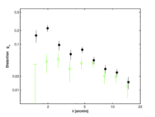
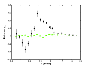
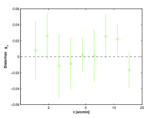
The tangential distortion of the green population behaves quite differently (Fig. 4) falling well below the background level near the cluster center. The green sample has a maximum signal at intermediate radius, $3\arcmin-5\arcmin$ , and then declines quickly inside this radius as the unlensed cluster galaxies dominate over the background in the center. Notice that the green sample does not fall to zero at the outskirts but rises up to almost meet the level of the background sample, indicating that the majority of the green sample at large radius comprises background rather than cluster members. We go on to use the ratio of the distortion of the green sample compared with the background level to determine the proportion of cluster members in § 6, but to do so we first evaluate the expected depths of our samples in § 5, in order to make a precise comparison of the lensing signals between them, since the lensing signal scales geometrically with increasing source distance and must be accounted for in any comparisons.

The results of this paper depend on the ratio of the background distortion to the cluster contaminated distortion, $(g_{T}^{(B)}/g_{T}^{(G)})$ , so that the 5-10% level calibration correction factors estimated from simulations done by the STEP project (Heymans et al., 2006) for the various weak distortion methods are not of major concern for the bulk of our work.

4. Distortion Analysis of ACS/HST images

In the center of the cluster inside a radius of approximately $1\arcmin$ the Subaru data become limited in depth by the extended bright haloes of the many luminous central galaxies. This region is far better resolved and more deeply imaged with HST/ACS in 20 orbits of imaging shared between the $g^{\prime}r^{\prime}i^{\prime}z^{\prime}$ passbands. Many multiple images are known here, defining accurately the shape of both the tangential and radial critical curves (Broadhurst et al., 2005a). Here we analyze the statistical distortion of the shapes of the many galaxies recorded in these images, to extend our analysis of the properties of the cluster galaxies into the center, allowing an accurately defined central cluster luminosity function to faint luminosities. In addition, it will be interesting to see how consistent the distortion profile derived here independently matches the mass profile obtained previously from the strongly lensed multiple images.

We stick to very similar definitions of the three-color selected population as with Subaru, but extend their depths by an additional $1^{m}.5$ magnitudes since the ACS data are so much deeper. The ACS images are limited to m=28.5 ( $5\sigma$ ) in each of the passbands. The reduction of the ACS image and the photometry for the faint sources is described in detail in Broadhurst et al. (2005a), including the subtraction of the bright central galaxies in the cluster which is essential for obtaining accurate photometry and shape measurements of central lensing images including radial arcs and demagnified central images. For the distortion analysis we prefer the im2shape method developed by Bridle et al. (2002) for dealing in particular with relatively elongated images produced by lensing in the strongly lensed region. This is an improvement over the standard KSB method which we used in the weak lensing regime appropriate for everything except the central region $r<2\arcmin$ , and used for the Subaru analysis described above.

Using this method, galaxies are fit to a sum of two sheared Gaussians convolved with a PSF. Each Gaussian has two free parameters, amplitude and width. The centroid and the shear are also allowed to vary, but these are restricted to be the same for both Gaussians. Meanwhile, the PSF for each galaxy is determined based on models described in Jee et al. (2005). These PSF models for ACS’s WFC were derived from observations of the globular cluster 47 Tuc (PROP 9656, P.I. De Marchi). As the distortion measurements are performed in the detection image, each galaxy is assigned an ”average” PSF based on the different filters and chip positions in which it was observed.

We plot the resulting values of $g_{T}(r)$ (Fig. 6) for the blue, green and red galaxies defined in the same color ranges as the Subaru data, but to fainter magnitudes. A very well defined saw-tooth pattern is visible, showing that images are maximally radially aligned at about $17\arcsec$ and then maximally tangentially aligned at about $47\arcsec$ . This is a very clear signature of strong lensing, where the maximum corresponds to the location of the tangential critical curve (Einstein radius), and the minimum to the radial critical curve, where images are maximally stretched in the radial direction generating a ring of long images pointing to the center of mass, as found in Broadhurst et al. (2005a). The location of these critical radii agrees very well with those derived from the model to the strong lensing data for this cluster, fitted by Broadhurst et al. (2005a).

Another clearly defined radius can also be identified from the point where the images distortion goes through zero, $g_{T}=0$ , at a radius in between these two critical radii at about $r\simeq 27\arcsec$ . It is important to note that in this region, between the two critical curves, the parity is $p=-1$ (odd parity), and here

g=\frac{1}{e^{*}}=\frac{e}{|e|^{2}}

(8)

(see Kaiser, 1995). Here, instead of measuring $g$ we are measuring $-1<e<1$ . (This is different than in the weak lensing region, outside the tangential critical curve, where $p=+1$ and $g=e$ , and therefore no distinction needed to be made). Since

e=\frac{1}{g^{*}}\propto 1-\kappa,

(9)

zero distortion corresponds to $\kappa=1$ curve, which lies in between the tangential and critical curves.

Note, for several reasons we cannot expect that the data will reach the theoretically extreme value of $g_{T}=1$ at the tangential critical radius, meaning that the images are infinitely stretched tangentially, and also $g_{T}=-1$ at the radial critical radius where they are stretched infinitely in the radial direction. By definition, weak lensing measurements will underestimate the sting distortions near critical curves. In addition, convolution by the redshift distribution of the background sources will smooth these features out. Nonetheless, we can define their locations in radius rather precisely and these positions must be reproduced in any satisfactory model, at $r\simeq 17\arcsec$ and $r\sim 48\arcsec$ . In addition the radius at which $g_{T}=0$ is also well defined at about $r\simeq 28\arcsec$ and corresponds to a surface density where $\kappa=1$ , supplying another important constraint on model mass profiles.

Outside the tangential critical curve we find that the tangential shear of the background sample (black circles in Fig. 6) drops to $g_{T,B}\sim 0.2$ at $r=2\arcmin$ , in good agreement with the Subaru analysis at this radius, giving us confidence in the consistency of our work. For the color range defined above, which includes the cluster sequence and all the bluer members of the cluster galaxy population, $g_{T,G}\sim 0$ over the full range of radius of the ACS data (green circles in Fig. 6), indicating - as expected - that the galaxy population in the this color range is dominated by cluster members with negligible background contamination.

5. Photometric Redshifts

We need to estimate the respective depths of our color-magnitude selected samples when estimating the cluster mass profile, because the lensing signal increases with source distance, and therefore must differ between the samples. The effect of this difference in distance on the weak lensing signal is simply linear as we can see from the relation between the dimensionless surface mass density,

\kappa(r)=\Sigma(r)/\Sigma_{crit},

(10)

where

\Sigma_{crit}=\frac{c^{2}}{4\pi Gd_{l}}\frac{d_{s}}{d_{ls}}

(11)

and the tangential distortion:

\langle g_{T}(r)\rangle=(\bar{\kappa}(r)-\kappa(r))/(1-\kappa(r))

(12)

so that in the weak limit where $\kappa$ is small,

\langle g_{T}(r)\rangle\propto{{d_{ls}\over{d_{s}}}{(\bar{\Sigma}(r)-\Sigma(r))}}

(13)

and hence for an individual cluster, with a fixed redshift and a given mass profile, the observed level of the weak distortion simply scales with the lensing distance ratio. Further details are presented in the appendix. The mean ratio of $d_{ls}/d_{s}$ , which is weighted by the redshift distribution of the background population corresponding to our magnitude and color cuts, is calculated using the expression

\langle D\rangle\equiv\langle{d_{ls}\over{d_{s}}}\rangle=\frac{\int{\displaystyle{d_{ls}\over{d_{s}}}(z)N(z)dz}}{\int{N(z)dz}}.

(14)

Since we cannot derive complete samples of reliable photometric redshifts from our limited 2-color V,i’ images of A1689, we instead make use of other deep field photometry covering a wider range of passbands, sufficient for photometric redshift estimation of the faint field redshift distribution appropriate for samples with the same color and magnitude limits as our red, green and blue populations.

The photometry of Capak et al. (2004) is very well suited for our purposes, consisting of relatively deep multi-color photometry over a wide field taken with Subaru, producing reliable photometric redshifts for the majority of field galaxies to faint limiting magnitudes. The Capak et al. (2004) galaxy catalog contains almost 50,000 galaxies over $0.2$ sq. deg. with $UBVRIZ$ photometry. We have estimated photometric redshifts for this catalog using the Bayesian based method of Benítez (2000), with a prior based on the redshift and spectral type distributions of the HDF-N, with a spectral library containing the templates of Benítez et al. (2004) with an additional two blue starburst galaxies as described in Coe et al. (2006).

A full redshift probability distribution is produced for each galaxy of the form:

p(z|C)\propto\sum_{T}p(z,T|m_{0})p(C|z,T),

(15)

where $p(C|z,T)$ is the redshift likelihood obtained by comparing the observed colors $C$ with the redshifted library of templates $T$ . The factor $p(z,T|m_{0})$ is a prior which represents the redshift/spectral mix distribution as a function of the observed $I-$ band magnitude. We use a prior which describes the redshift/spectral type mix in the HDF-N, which has been shown to significantly reduce the number of “catastrophic” errors ( $\Delta z>1$ ) in the photometric redshift catalog (see Benítez et al., 2004, and references therein). For each galaxy we look at its redshift probability distribution p(z) and identify up to 3 redshift local maxima. Each of these maxima corresponds to a redshift $z_{i}$ , spectral type $t_{i}$ , and a discretized probability $p_{i}(z_{i},t_{i})\leq 1$ . Using this information we generate a mock observation of all the $z_{i},t_{i}$ combinations in the Subaru filters, and then build a redshift histogram by selecting galaxies using the same color cuts and adding up their probabilities in each redshift bin.

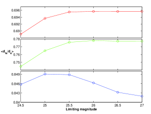
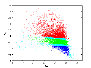
The color-magnitude diagram for the Capak catalog galaxies is shown in Figure 7, where the equivalent color-magnitude selected samples are displayed. The resulting mean redshift of the background galaxies in each of our three color-selected samples is caclulated as a function of limiting magnuite of the sample (Fig. 9), by using the redshift distribution from the Capak catalog. The redshift distribution is also used to evaluate the weighted mean depths $\langle D\rangle$ (shown in Fig. 8 as a function of sample limiting magnitude), for comparing the weak lensing amplitudes between the green and the red+blue samples. This is done by dividing up each sample into 81 independent bins of $2\arcmin$ , calculating the weighted mean redshift and depth in each, and taking the mean value and variance over the bins. The mean redshift of the red sample is only $\langle z_{red}\rangle\sim 0.871\pm 0.045$ , whereas the blue sample is calculated to have, $\langle z_{blue}\rangle\sim 2.012\pm 0.124$ . The green sample lies in between with, $\langle z_{green}\rangle\sim 1.429\pm 0.093$ . The weighted relative depths of these samples using equation (14), for samples selected to our magnitude limit of $i<26.5$ , are $\langle D_{red}\rangle=0.693\pm 0.012$ , $\langle D_{green}\rangle=0.728\pm 0.012$ , and $\langle D_{blue}\rangle=0.830\pm 0.011$ , and the corresponding redshifts $z_{D}$ equivalent to these mean depths are, $z_{D,red}=0.68$ , $z_{D,green}=0.79$ , $z_{D,blue}=1.53$ , respectively. Hence the ratio of the mean depth of the blue sample to the red sample is $\langle D_{blue}\rangle/\langle D_{red}\rangle=1.20$ , accounting well for the observed offset seen in Figure 3.

We also make use of the Capak “green” sample to investigate the level of “cosmic variance” in $d_{ls}/d_{s}$ , and although there is variation in the redshift distribution the variance of the mean redshift is remarkably tight, and as quoted above we find a very small variance associated with the mean lensing depth, $\sigma(\langle{}d_{ls}/d_{s}\rangle{})=0.015$ . This stability is also a feature noticed in pencil beam redshift surveys in general, that the mean depth is stable to spikes in the redshift distribution, e.g., Broadhurst et al. (1988).

The form of the distance ratio $D$ can be expressed in terms of the redshifts of the source and lens for a given set of cosmological parameters. In the main case of interest, that of a flat model with a nonzero cosmological constant, the relation is given by

	$\displaystyle{d_{ls}\over{d_{s}}}$	$\displaystyle=$	$\displaystyle 1-\frac{(1+z_{l})^{2}\zeta(z_{l})}{(1+z_{s})^{2}\zeta(z_{s})}$		(16)
	$\displaystyle\zeta(x)$	$\displaystyle=$	$\displaystyle\int^{x}_{0}\frac{dz}{[\Omega_{\Lambda}+\Omega_{M}(1+z)^{3}]^{1/2}}.$		(17)

General expressions for the dependence of this distance ratio on arbitrary combinations of $\Omega_{M}$ and $\Omega_{\Lambda}$ are lengthy and can be found in Fukugita et al. (1990). For a low redshift cluster like A1689 (z=0.183), the form of this function is rather flat for sources at $z>1$ , see Broadhurst et al. (2005a). Therefore the main uncertainty in determining the cosmological parameters from a comparison of $g_{T}$ between samples of different redshifts, is small compared with clustering noise along a given line of sight behind the cluster, as examined in detail by (Broadhurst et al., 2005a). Thus, we do not seriously examine this effect here but rather simply adopt the recent (three year) WMAP cosmological parameters (Spergel et al., 2006) when making the above depth correction. With sufficient number of clusters and similar or better photometric redshift information (from multiple filter observations) one can hope to examine the trend of redshift vs. lensing distance in the future.

Note that lensing magnification, $\mu$ , will modify $g_{T}$ slightly by increasing the depth to a fixed magnitude. But the magnification is small, $\mu<0.^{m}2$ over most of the cluster, $r>3^{\prime}$ . In any case, the dependence of the mean redshift on depth is a slow function of redshift, so that it is safe for our main purposes to ignore the effect of magnification on the depth of our samples. Furthermore, since we are only interested in the proportion of the cluster relative to the background for our purposes, we are not affected by the modification of the background number counts caused by lensing, which has been shown to significantly deplete the surface density of background red galaxies in A1689, and found to be consistent with the predicted level of magnification based on the distortion measurements (Broadhurst et al., 2005b).

6. Weak Lensing Dilution

We can now estimate the number density of cluster galaxies by taking the ratio of the weak lensing signal between the green sample and the background sample, with the background including both red and blue galaxies selected from the Subaru catalog as explained in § 2, and accounting for differences in the relative depths of these samples, as explained in § 5.

Cluster members are unlensed and hence assumed to have random orientations, so they are expected to contribute no net tangential lensing signal. This assumption can be examined for the brighter ( $i^{\prime}<21^{m}.5$ ) cluster sequence galaxies whose tight sequence protrudes beyond the faint field background (Fig. 1) with negligible background contamination, so that we are secure in selecting this subset to test the assumption that the cluster galaxies are randomly oriented. Indeed, the net tangential signal of this population is consistent with zero (Fig. 10), $g_{T}^{(G)}=0.0043\pm 0.0091$ .

For a given radial bin ( $r_{n}$ ) containing objects in the green sample, whose width in color has been chosen to encompass the full range of cluster galaxies (§ 2), the mean value of $g_{T}^{(G)}$ (eq. 6) is an average over background and cluster members. Thus, its mean value $\langle g_{T}^{(G)}\rangle$ will be lower than the true background level denoted by $\langle g_{T}^{(B)}\rangle$ (Fig. 4) in proportion to the fraction of unlensed galaxies in the bin that lie in the cluster (rather than in the background), since the cluster members on average will add no net tangential signal. Therefore,

f_{cl}(r_{n})\equiv\frac{N_{cl}}{N_{Green}}=1-\frac{\langle{}g_{T}(r_{n})^{(G)}\rangle{}}{\langle{}g_{T}(r_{n})^{(B)}\rangle{}}\frac{\langle D^{(B)}\rangle}{\langle D^{(G)}\rangle}

(18)

is the cluster membership fraction of the green sample (see full derivation in the appendix).

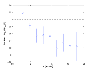
Thus, we can use this effect to quantify statistically the number of cluster galaxies by comparing $g_{T}^{(G)}$ with the true background level derived from the pure background red and blue samples $g_{T}^{(B)}$ , at a fixed radius. This is shown in Figure 11, where we have also taken into account the effect of the relative depths of the differing samples. We find that the fraction of cluster members drops smoothly from $\sim 100\%$ within $r<2\arcmin$ to only $\sim 20\%$ at the limit of the data, $r\sim 15\arcmin$ .

7. Cluster light and color profiles

To determine the luminosity profile of the cluster galaxies, we need to go further, because in general the brightness distribution of the cluster members is different than that of the background galaxies; specifically, it is skewed to brighter magnitudes, certainly for the bulk of the cluster sequence. To account generally for any difference in the brightness distributions we can subtract a “ $g_{T}$ -weighted” luminosity contribution of each galaxy, which when averaged over the distribution will have zero contribution from the unlensed cluster members. We first calculate the “g-weighted” correction in arbitrary flux units. We estimate the total flux of the cluster in the $n^{th}$ radial bin,

F_{cl}(r_{n})=\displaystyle\sum_{i}{F_{i}^{(G)}}-\frac{\langle{}D^{(B)}\rangle{}/\langle{}D^{(G)}\rangle{}}{\langle{}g_{T}(r_{n})^{(B)}\rangle{}}\displaystyle\sum_{i}{F_{i}^{(G)}\cdot{}g_{T,i}^{(G)}}

(19)

where the sum is over all galaxies in the radial bin.

The flux is then translated back to apparent magnitude, and from that the luminosity is derived. First we calculate the absolute magnitude,

M_{i^{\prime}}=i^{\prime}-5\log{d_{L}}-K(z)+5,

(20)

where the $K$ -correction is evaluated for each radial bin according to its $V-i^{\prime}$ color, which - after the correction is made for each of the bands - is now the cluster color. The luminosity is then

L_{i^{\prime}}=10^{0.4(M_{i^{\prime}\odot}-M_{i^{\prime}})}L_{i^{\prime}\odot},

(21)

where $M_{i^{\prime}\odot}=4.54$ is the absolute $i^{\prime}$ magnitude of the Sun (AB system).

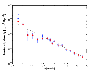
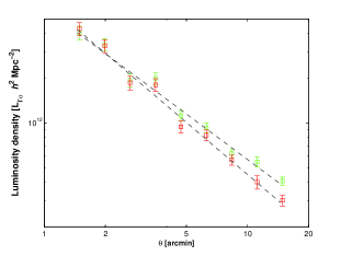
The result yields the luminosity profile of the cluster as shown in Figure 12 (red squares). Here we can see that the cluster luminosity profile is well approximated by a simple power-law with a projected slope of $d\log(L_{i^{\prime}})/d\log(r)\sim-1.12\pm 0.06$ , to the limit of the data. We also show in Figure 13 the unweighted luminosity profile with no correction for the field, demonstrating that the g-weighted correction is negligible at small radius as expected, since the cluster dominates numerically over the background, but becomes increasingly more important at larger radius where the background dominates. Note that we derive a more accurate inner luminosity profile using the ACS photometry for the central region (Fig. 12, red circles), and here there is only a negligible correction for the background due to the high central density of galaxies in this cluster.

In a careful study of clusters and groups identified in the SDSS survey, Hansen et al. (2005) find a similar slope for the most massive clusters, in terms of the composite surface density profile of $d\log(n)/d\log(r)\simeq-1.05\pm 0.04$ , over the radius range $r<2$ Mpc, with slightly shallower slopes occurring in the less overdense clusters and groups. This may be compared directly with our slope derived above, assuming a constant $M_{*}/L$ , for the ratio of galaxy mass to galaxy luminosity. More directly we derive a density profile using the $f_{cl}n^{(G)}$ which also gives a slope of $\simeq-0.9\pm 0.09$ .

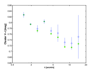
In the same manner, we construct a “g-weighted” color profile of the cluster, $V-i^{\prime}$ , which we have corrected as described above. We obtain a color profile that shows a weak tendency towards bluer colors with increasing radius, as expected, indicating a tendency towards later-type galaxies at large radius (Fig. 14). Also shown is the unweighted color profile (green points), which again is steeper due to the uncorrected field component which dominates numerically over the cluster at larger radius and is generally bluer in color than the cluster. This change in color with radius corresponds to a significant radial gradient in spectral type, from predominantly early-type with $(V-i^{\prime})_{AB}\simeq 0.84$ , to mid sequence type, Sb, with $(V-i^{\prime})_{AB}\simeq 0.73$ , and indicates that for this cluster very blue starburst and Scd galaxies are not the dominant population at the limiting radius of our sample ( $r\sim 2~{}h^{-1}$ Mpc), where otherwise the color would tend to $(V-i^{\prime})_{AB}\simeq 0.5$ , using standard template sets (Benítez et al., 2004). We go on to make use of this color-radius relation in § 9, when examining the radial profile of the ratio of total cluster mass to the stellar mass in galaxies. We do this by correcting the luminosity profile for the tendency towards more luminous early-type stars that are responsible for the bluer galaxy colors at large radius and which otherwise bias the interpretation of the $M/L$ ratio, as described below.

8. Cluster Luminosity Functions

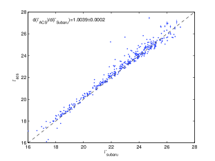
The data allow the luminosity function to be usefully constructed in several independent radial and magnitude bins, and hence we can examine the form of the luminosity function of cluster members as a function of projected distance from the cluster center. For this we combine the ACS and the Subaru photometry. The ACS has the advantage of extending two magnitudes fainter in the $i^{\prime}$ -band than the Subaru photometry for $r<2\arcmin$ . As can be seen in Figure 15, the ACS $i^{\prime}$ magnitudes agree with Subaru $i^{\prime}$ magnitudes for galaxies found and matched in both catalogs.

The background correction to evaluate $f_{cl}$ , must be made in each magnitude bin independently, since the relative proportion of background galaxies increases with apparent magnitude, so that the lower luminosity bins of the green luminosity function are expected to contain a greater fraction of background galaxies and hence should have a relatively higher value of $g_{T}^{(G)}$ . This trend is apparent in Figure 16 (left panels), where we plot the recovered mean tangential distortion (here the average is over a magnitude bin) for each of the four radial bins, as a function of absolute magnitude. A clear trend is found at all radii towards higher levels of $g_{T}$ at fainter luminosities. Note that the mean level of the background distortion (black solid line) drops with increasing radius so that the proportion $g_{T}^{(G)}(M)/g_{T}^{(B)}$ is generally an increasing function of radius and a decreasing function of luminosity. To correct for this we simply apply equation (18) to each magnitude bin:

\Phi_{cl}(M_{k})=\Phi(M_{k})\cdot[1-\langle{}g_{T}^{(G)}(M_{k})\rangle{}/\langle{}g_{T}^{(B)}(r)\rangle{}]

(22)

(Note that the background signal is averaged over the whole range of magnitudes at that radius.)

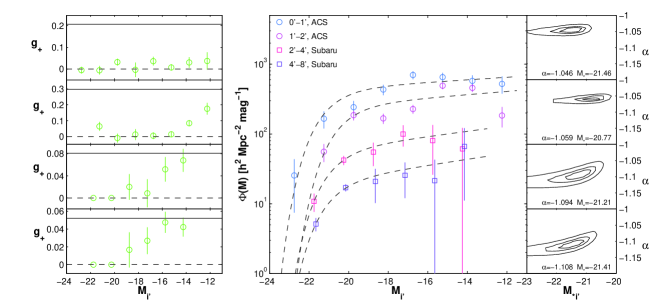
We then construct the luminosity function for four independent radial bins, as shown in Figure 16 (middle panel) and fit a Schechter (1976) function to each (dashed lines). It can be seen that there is no obvious tendency for the shape of the luminosity function to change with radius. The faint-end slope of a Schechter function fit is $\alpha=-1.05\pm 0.07$ in the $i^{\prime}$ -band. This constancy with radius has been argued with somewhat less significance in other well studied massive clusters (e.g., Pracy et al., 2005), based on similar deep 2-color imaging, where the limiting radius is more restricted. We also construct a composite luminosity function for the whole cluster (Fig.17), for $r<10\arcmin$ , which shows clearly the effect of our “g-weighted” background correction, without which the faint-end slope would be considerably steeper, $\alpha\sim 1.4$ .

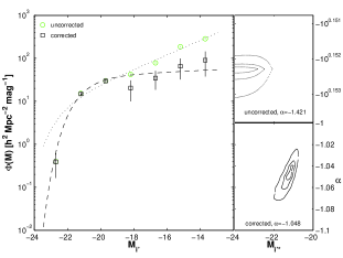
Our approach is of course essentially free of uncertainties in the subtraction of background galaxies by its nature. While qualitative similarity between the results of the various studies is clear, agreement in detail is not necessarily expected, given the likely dispersion in the strength of this effect between clusters. Also, the question of background contamination is always an issue in the standard approach due to the inherent fluctuations in the surface density of background galaxies, and the need to establish the background counts at a sufficiently large radius from the cluster to avoid self-subtraction of the cluster at the boundaries of the data, a subject explored in depth, e.g. Adami et al. (2000); Paolillo et al. (2001); Andreon et al. (2005); Hansen et al. (2005); Popesso et al. (2005).

We also integrate our luminosity functions as a consistency check of the luminosity density profiles derived earlier. This is done by calculating $\Phi_{cl}(M)$ in the same radial bins as our luminosity profile above, and summing over the magnitude bins:

L_{cl}(r_{n})=\displaystyle\sum_{k}\Phi_{cl}(M_{k})\cdot\Delta M_{k}\cdot 10^{0.4(M_{i^{\prime}\odot}-M_{k})}

(23)

The results shown above in Figure 12 (blue points) agree very well with those of $L_{cl}$ described in the previous section.

Note that in constructing these luminosity density profiles we have implicitly assumed that the luminosity function is integrated over fully. Fortunately our data is complete to a sufficient depth ( $i^{\prime}<26.5$ ) so that the contribution of the integrated luminosity density from undetected objects is very small, as evaluated when we examine the luminosity functions. The difference between integrating up to a limiting magnitude of $M_{i^{\prime}}<-14$ and extrapolating up to $M_{i^{\prime}}<-10$ is only about $0.1\%$ .

The lack of any obvious upturn in the cluster luminosity function to very faint luminosities, $M_{i^{\prime}}<-12$ , in the cluster core, is in agreement with several other studies based on deep photometry of large cluster samples, e.g., the composite cluster luminosity function derived by Gaidos (1997); Garilli et al. (1999); Paolillo et al. (2001); Hansen et al. (2005); Pracy et al. (2005), where wide field imaging is employed for several Abell clusters and overdensities identified in the SDSS survey, and where careful attention can be paid to the background counts and their uncertainty. The study of Pracy et al. (2005) is the most similar to our own, containing three rich and fairly distant Abell clusters, and here the LF’s show no obvious upturn to $M<-13$ with a generally flat Schechter function slope in the range -1.1 to -1.25.

For the well studied Coma cluster, a steeper slope has been claimed, $\alpha\simeq-1.4$ , by Bernstein et al. (1995), though subsequent faint spectroscopy by Adami et al. (2000), has revealed the presence of a background cluster at $z\simeq 0.5$ , which when corrected for leads to a flat faint-end slope. In contrast an upturn is claimed for a composite sample of 25 SDSS selected clusters by Popesso et al. (2005), though an individual examination shows considerable variation, with only a minority of $\sim 6$ displaying a distinct upturn which varies in amplitude, so that one may wonder about the role of anomalous background count fluctuations in these cases.

9. $M/L$ profiles

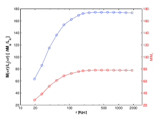
We may now go on to examine the mass-to-light ratio using the mass profile previously determined based on the distortion and magnification profile of the red galaxy sample, as derived by Broadhurst et al. (2005b), and also based on the central strong lensing information derived from 106 multiple-images (Broadhurst et al., 2005a). The mass profile derived in Broadhurst et al. (2005b) was found to be somewhat more pronounced than a simple NFW form, with the observed gradient increasing monotonically with radius from the cluster center. Dividing the mass profile by our newly derived light profile we obtain a profile of the mass-to-light ratio for A1689 as shown in Figure 18.

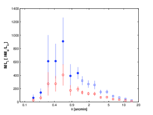
We find that the $M/L$ ratio peaks at intermediate radius around $2\arcmin$ ( $r\sim 100~{}h^{-1}$ Kpc) and then falls off linearly to larger radius. (Broadhurst et al., 2005a) have previously identified the drop in $M/L$ at small radius as due principally to the tight central clump of very luminous cluster members, noting that this clump may have resulted from the effect of dynamical friction.

Note that the peak value is rather large, equivalent to $M/L_{B}\sim 400h(M/L)_{\odot}$ in the restframe B-band often used as a reference, but the mass of A1689 is at the extreme end of the cluster population, $M\sim 2\times 10^{15}hM_{\odot}$ (Broadhurst et al., 2005b), and given the general tendency of $M/L$ to increase with increasing mass, from galaxies through groups to clusters, we may not be surprised to find the peak to somewhat exceed the typical range for clusters, $150-300h{M/L_{B}}_{\odot}$ (Carlberg et al., 2001). The general profile of $M/L$ is similar in form to that derived for CL 0152-1357 by Jee et al. (2005) based on a careful weak lensing analysis of recent deep ACS images.

We have also constructed a profile of the total mass to stellar mass $M/M_{*}$ ratio. This is arguably a more physically useful indicator of the relationship between dark and luminous matter compared to the ratio of $M/L$ , because the starlight can be strongly influenced by the presence of relatively small numbers of luminous hot stars. To calculate $M/M_{*}$ we make use of the color profile derived in § 7, and an empirical relationship between color and the ratio $M_{*}/L$ for stellar populations established for local galaxies in the the SDSS survey by Bell et al. (2003). The slope of the projected stellar mass profile, $d\log M_{*}/d\log r=-1.15\pm 0.13$ , derived this way is slightly steeper than the luminosity profile, as expected. The observed relation we derive this way is somewhat flatter than for $M/L$ and the mean contribution by mass for stars is about $1.25\%$ for this cluster and similar to a mean value of $\sim 2\%$ derived from a carefully selected sample of local clusters by Biviano & Salucci (2006).

10. Cluster Mass Profile

We use the combined distortion information obtained from the ACS and Subaru imaging, as described above (Fig. 6) and compare with models for the mass distribution. We have improved on our earlier distortion measurements made with Subaru, with the addition of the background blue galaxy population defined here, so that the significance of the distortion measurements is somewhat greater than our earlier work which was based only on the red sample (Broadhurst et al., 2005b). In addition, we have extended the distortion measurements to the central region using the HST/ACS information, as described in § 4, where we have clearly identified a maximum and a minimum value of $g_{T}$ , which accurately correspond to the tangential and radial critical curves (Fig.20), independently derived from the the many giant tangential and radial arcs observed for this cluster (see Broadhurst et al., 2005a).

Here we test the universal parameterization of CDM-based mass profiles advocated by Navarro et al. (1997). This model profile is weighted over the differing results from sets of haloes identified in N-body simulations. A cluster profile is summed over all the mass contained within the main halo, including the galactic haloes. Hence, we compare the integrated mass profile we deduced directly with the NFW predictions without having to invent a prescription to remove the cluster galaxies.

NFW have shown that massive CDM haloes are predicted to be less concentrated with increasing halo mass, a trend identified with collapse redshift, which is generally higher for smaller haloes following from the steep evolution of the cosmological density of matter. The most massive bound structures form later in hierarchical models and therefore clusters are anticipated to have a relatively low concentration, quantified by the ratio $C_{vir}=r_{virial}/r_{s}$ . In the context of this model, the predicted form of CDM dominated are predicted to follow a density profile lacking a core, but with a much shallower central profile ( $r\leq 100~{}h^{-1}$ kpc) than a purely isothermal body.

The fit to an NFW profile is made keeping $r_{s}$ , and $\rho_{s}$ , the characteristic radius and the corresponding density, as free parameters. These can be adjusted to normalize the model to the observed maximum in the distortion profile at the tangential critical radius of $\simeq 45\arcsec$ . The combination of these parameters then fixes the degree of concentration, and the corresponding lensing distortion profile can then be calculated.

Integrating the mass along a column, z, where $r^{2}=({\xi_{r}}{r_{s}})^{2}+$ z² gives:

{M}(\xi)={\rho_{s}}{r_{s}^{3}}(\xi)\int_{o}^{\xi}d^{2}\xi\int_{-\infty}^{\infty}{\frac{1}{(r/r_{s})(1+r/r_{s})^{2}}}{\rm{dz}\over{r_{s}}}.

(24)

Using this mass, a bend-angle of $\alpha=\frac{4GM(<\theta)}{c^{2}\theta{d_{l}}}\frac{d_{ls}}{d_{s}}$ is produced at position ${\theta}=\xi r_{s}/d_{l}$ . The mean interior mass within some radius $r_{x}=xc_{x}r_{s}$ can be obtained by integration of the NFW profile giving:

M(<r)={4\pi\over{3}}r_{x}^{3}{\Omega_{m}(o)\Delta_{c}(1+z)^{3}\over{x^{3}\Omega_{m}(zl)}}{\left[{\log(1+xc_{x})-{xc_{x}\over{1+xc_{x}}}\over{\log(1+c_{x})-{c_{x}\over{1+c_{x}}}}}\right]},

(25)

where the above integral is carried out to the virial radius. Here when we make this comparison we do not attempt to fit the distortions in the region of the radial and tangential critical curves because the measurements must underestimate the amplitude of the model predictions near these curves due to the finite size of the background galaxies, so that the model maximum and minimum, $g_{T}=\pm 1$ corresponding to the tangential and radial critical curves cannot be reached by the data (see Fig. 6) near these critical curves. Finite area sources are on average not as magnified or distorted as an ideal point source due to the gradient of the lensing magnification over the surface of the source, so that for a source lying over a lens caustic only an infinitesimally small area is infinitely magnified. In principle simulations based on realistic galaxy samples like those modeled by Bouwens et al. (1998) could be used to correct for this effect but this will await further work.

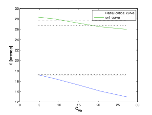
We can instead utilize here the observed location of these critical curves since a clear maximum and minimum is observed in the inner distortion data (Fig. 6) and has also been independently determined from the multiple-image data (Broadhurst et al., 2005a) for this cluster. In addition to the location of the critical curves we can also clearly identify the radius where $g_{T}=0$ , lying in between these critical curves. At this radius the radial and tangential magnifications are equal and hence images are unchanged in shape (though in general highly magnified), so the observed value of $g_{T}$ will pass through zero at a radius in between the critical curves. This radius corresponds to the contour where the projected surface density is equal to the critical surface density, $\Sigma=\Sigma_{crit}$ (e.g., Kaiser, 1995), and hence is smaller for more concentrated profiles. In Figure 20 we plot these two radii as a function of model concentration, where the models are all normalized to a tangential critical radius of $47\arcsec$ to match the mean critical radius derived from the data (Broadhurst et al., 2005a).

To normalize the models we choose to reproduce the observed Einstein radius of $47\arcsec$ and compare the predicted location of the radial critical curve and the $\kappa=1$ curve. Figure 20 shows that both these radii decrease slowly as the concentration parameter is increased. We have marked the observed values of these radii as determined by two independent observational means. We can use the statistical distortion measurements as described in § 3, and the same values derived from the multiple image analysis presented in Broadhurst et al. (2005a). These differing estimates are closely consistent with each other, and by comparison with the model curves bracket intermediate values of concentration in the range $5<C_{vir}<15$ (Fig. 20), a range consistent with the results from a detailed fit to the inner profile measured in Broadhurst et al. (2005a). This is found to be very similar to the independently derived central profile of A1689 from Diego et al. (2005); Zekser et al. (2006); Halkola et al. (2006).

Outside the tangential critical radius, for $r>1.5$ , the distortion measurements are small enough not to suffer from any significant underestimation due to the finite source sizes and we may compare the observed distortion profile, $g_{T}(r)$ , out to the limit of our data, $r<15\arcsec$ . We find this distortion profile is reasonably well fitted by an NFW profile particularly at large radius, $4.0\arcsec<r<15\arcsec$ , but with a relatively large concentration, $C_{vir}=27.2^{+3.5}_{-5.7}$ , as shown in Figure 21. Note that we have used here a linear radial binning when measuring the concentration parameter and therefore the result here is more weighted by large radius signal than for the analysis of Broadhurst et al. (2005b) where we used logarithmic binning, yielding a smaller value of $C_{vir}$ . This difference in the derived value of $C_{vir}$ is not becuase of any revision in our estimates of the distortion, in fact both analyses yield very consistent distortion profiles at large radius, but rather that the form of the NFW profile is not consistent with our data over the full radial range - the best fitting NFW model is either too shallow at large radius or too steep at small radius depending where one prefers to fit the data.

We also plot lower concentration profiles, including $C_{vir}=14$ , which was found previously by Broadhurst et al. (2005a), to fit best the overall lensing derived mass profile from combining the mass profile derived from the multiply lensed images in the central region, $r<2\arcmin$ , with the mass distribution derived from weak lensing distortion and magnification measurements from the red background galaxy sample. This model fit, as pointed out by Broadhurst et al. (2005b), is not as pronounced as the observed surface mass profile, being too shallow at larger radius and too steep at small radius (see figures 1&3 of Broadhurst et al., 2005b). Here we see more clearly that this fit with $C_{vir}=14$ increasingly overpredicts the observed distortion profile with radius. We also plot $C_{vir}=8.2$ which best fits the central strongly lensed region (Broadhurst et al., 2005a) $r<2\arcmin$ , derived from 106 multiply lensed images. Again this fit overpredicts the $g_{T}$ profile in the weak lensing regime, as pointed out in Broadhurst et al. (2005b).

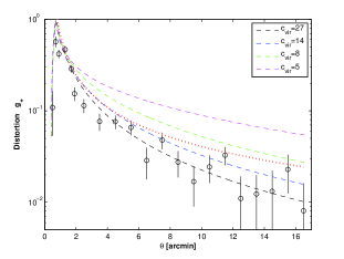
We clearly exclude the low concentration profile generally predicted by CDM based models of structure formation. A value of $C_{vir}\sim 5$ is generally anticipated for massive clusters, although the scatter in concentration at a given mass is considerable (e.g., Bullock et al., 2001). Figure 21 shows clearly how this profile is much too shallow to generate the relatively steeply declining observed distortion profile. The triaxiality of realistic haloes means that projection effects will bias somewhat the derived distortion profile, as examined carefully by Oguri et al. (2005) and Hennawi et al. (2005), showing that the level of such bias effect is expected to enhance the derived concentration by approximately $\sim 20\%$ on average. Whilst A1689 is clearly an anomalous cluster in terms of the size of the Einstein radius, the cluster is very round in terms of the projected X-ray emission, with only minimal substructure observed in the optical near the center. Hence we are left with a clearly unresolved problem, that the observed concentration would seem to far exceed any reasonable estimate. Other independent work on the combined profile from strong and weak lensing measurements for the clusters Cl0024+17 (Kneib et al., 2003) and MS2137-23 (Gavazzi et al., 2003) also point to surprisingly high concentrations, and it is therefore important to extend this type of detailed work to other clusters to test the generality of the profile derived here.

For reference we also plot the distortion profile for a singular isothermal body in Figure 21, which is simply expressed as

g_{T}=\frac{1}{2\frac{\theta}{\theta_{E}}-1},

(26)

and normalized to the observed Einstein radius, $\theta_{E}=47\arcsec$ . This model also overpredicts the data at large radius, indicating the outer mass profile is steeper than $1/\theta$ in projection.

11. Discussion and Conclusions

We have explored a new approach to deriving the luminous properties of cluster galaxies by utilizing lensing distortion measurements, based on the dilution of the lensing distortion signal by unlensed cluster members which we assume are randomly oriented. We have tested this assumption for a restricted sample of bright cluster galaxies which project beyond the faint galaxy background population so the level of background contamination is negligible, confirming that the cluster galaxies are randomly oriented with a negligible net tangential distortion for the purposes of our work.

This dilution approach is applied to A1689 to derive the radial light profile of the cluster, a color profile and radial luminosity functions. The light profile is found to be smoothly declining and fitted with a power-law slope $d\log(L)/d\log(r)=-1.12\pm 0.06$ . We also see a mild color gradient corresponding to a change in the cluster population from early- to mid-type galaxies in moving from the center out to the limit of our data at 2 $h^{-1}$ Mpc. Unlike the light profile the gradient of mass profile is continuously steepening, such that the ratio of $M/L$ peaks at intermediate radius. We find that the cluster luminosity function has a flat faint-end slope of $\alpha=-1.05\pm 0.07$ , nearly independent of radius and with no faint upturn to $M_{i^{\prime}}<{-12}$ .

A major advantage of our approach is that we do not need to define far-field counts for subtracting a background, as in the usual method where there is a limitation imposed by the clustering of the background population that limits the radius to which a reliable subtraction of the background can be made.

We have also established that the bluest galaxies in the field of A1689 lie predominantly in the background, as their radial distortion profile follows closely the red galaxies, but with an offset indicating the blue population lies at a greater mean distance than the red background galaxies, and consistent with the estimated mean redshifts of these two populations. With a larger sample of clusters, this purely geometric effect can potentially be put to use to provide a simple model-independent measure of the cosmological curvature.

The mass profile of A1689 was reexamined using our combined background sample of red and blue galaxies. The distortion profile derived from this sample is consistent with our earlier work, but somewhat more statistically significant, so we have examined the mass profile more carefully out to a larger radius. We have found that the distortion profile is steeper than predicted for CDM haloes appropriate for cluster sized masses $C_{vir}\sim 5$ . This discrepancy is particularly clear at large radius $r>2\arcmin$ , where an acceptable fit is found to an NFW profile but with a concentration $C_{vir}=27^{+3.5}_{-5.7}$ . This finding is consistent with our earlier work which showed that although an overall best fit profile of $C_{vir}\simeq 14$ to the joint strong and weak lensing based data presented in Broadhurst et al. (2005b), the curvature of the data is more pronounced than an NFW profile being shallower in the inner region and steeper at larger radius, so that the derived value of the concentration increases with radius depending on the radial limits being examined.

This result is surprising and may require a significant departure from the standard CDM model, either in terms of the mass content, or the epoch at which the bulk of the cluster was assembled. For example, one possibility to achieve earlier formation of clusters is to allow deviation from Gaussianity of the primordial density fluctuation field, as has been considered recently by, e.g., Sadeh et al. (2006). A1689 is amongst the most massive known clusters, and projection effects may play a role in boosting somewhat the lensing signal along the line of sight. We therefore aim to test the generality of this result with a careful study of a statistical sample of clusters.

Upcoming spatially resolved SZ measurements will add a significant new ability to determine cluster mass profiles over a large range of radius, and allow for improved consistency checks between the various independent means of estimating masses. The combination of X-ray, lensing and SZ measurements will soon lead to far greater accuracy in understanding the nature of cluster mass profiles.

We plan an improvement to the weak lensing work with deeper multi-color imaging from Subaru for measuring reliable photometric redshifts for a sizable fraction of the background population. This added dimension of depth will enhance the weak lensing signal and reduce the systematic problems of cluster and foreground contamination of the lensing signal. We also aim to extend this work to well studied clusters at lower redshift with archived Subaru imaging and detailed X-ray and upcoming SZ observations as in principle, the lensing signal should be equally strong for lower redshift clusters, given the maximal ratio of lens to source distances, $d_{ls}/d_{s}\simeq 1$ , for faint background sources.

We are grateful to N. Kaiser for making the IMCAT package publicly available. We thank Masahiro Takada, Doron Lemze and Eran Ofek for useful discussions and in addition we thank Eran Ofek for useful Matlab routines. We thank our referee Raphael Gavazzi for a thorough reading of the manuscript and many useful suggestions. TJB thanks the generosity of the JSPS and the hospitality of NAOJ and the Astronomical Institute of Tohoku University. ACS was developed under NASA contract NAS5-32865, and this research was supported in part by NASA grant NAG5-7697. Work at Tel-Aviv University was supported by Israel Science Foundation grant 214/02.

Appendix A Appendix A: Cluster Galaxy Fraction from the Lensing Dilution Effect

Let us derive eq. (18). For simplicity, here we assume the weak lensing limit so that the reduced shear is approximated by the gravitational shear, $g\approx\gamma$ . It is useful to factorize the lensing signal with the geometry-dependent factor such that (Seitz & Schneider, 1997):

g_{T}(r)=w(z)g_{T,\infty}(r)

(A1)

where $g_{T,\infty}(r)$ denotes the tangential shear calculated for hypothetical sources at an infinite redshift, and $w(z)$ is the lensing strength of a source at $z$ relative to a source at $z\rightarrow\infty$ , $w(z)=D(z)/D(z\to\infty)$ ; $D(z)\equiv d_{ls}/d_{s}$ as introduced in §5. The relative lensing strength vanishes for cluster and foreground galaxies, that is, $w(z)=0$ for $z\leq z_{l}$ .

As the tangential shear is obtained by averaging over an annular region, it can be formally written in the following form:

\langle g_{T}(r)\rangle=g_{T,\infty}(r)\frac{\int d^{2}x~{}dz~{}dn/dz~{}w(z)}{\int d^{2}x~{}dz~{}dn/dz}=g_{T,\infty}(r)\frac{\int_{z_{l}}^{\infty}dz~{}dN/dz~{}w(z)}{N_{tot}}=g_{T,\infty}(r)\frac{N_{bg}}{N_{tot}}\langle w\rangle_{z>z_{l}}

(A2)

where $dn/dz$ is the surface number density distribution of galaxies per unit redshift interval per steradian, $dN/dz=\int d^{2}x~{}dn/dz$ is the mean redshift distribution of galaxies in the annulus, $N_{tot}=\int_{0}^{\infty}\!dz~{}dN/dz$ is the total number of galaxies in the annulus, $N_{bg}=\int_{z_{l}}^{\infty}\!dz~{}dN/dz$ is the number of background galaxies in the annulus, $\langle w\rangle_{z>z_{l}}=\int_{z_{l}}^{\infty}\!dz\,dN/dz~{}w(z)/\int_{z_{l}}^{\infty}\!dz\,dN/dz$ is the mean lensing strength without including the dilution effect; here we have assumed that the lensing properties are constant over the annulus where we take the ensemble averaging. Note that the factor $N_{bg}/N_{tot}$ accounts for the dilution effect on the lensing signal strength due to contamination by foreground and cluster-member galaxies. In general, there is a contribution from foreground galaxies to the total number of galaxies $N_{tot}$ . However, for the case of A1689 at a low redshift of $z_{l}=0.183$ , this contribution is negligible. That is, $N_{\rm tot}\approx N_{cl}+N_{bg}$ with $N_{cl}$ being the number of cluster galaxies in the annulus. For a background galaxy sample, $N_{tot}=N_{bg}$ .

Since we are to compare galaxy samples with different redshift distributions, we need to account for different values of the mean lensing strength, $\langle w\rangle_{z>z_{l}}$ . As explained above, our green sample (denoted with G) comprises both cluster and background galaxies. Hence, according to eq. (A2), the expectation value for the mean tangential shear estimate is

\langle g_{T}^{(G)}(r)\rangle=g_{T,\infty}(r)\frac{N_{bg}^{(G)}}{N_{cl}+N_{bg}^{(G)}}\langle w^{(G)}\rangle_{z>z_{l}}.

(A3)

As for our background sample (denoted with B), including the red and blue samples, this is

\langle g_{T}^{(B)}(r)\rangle=g_{T,\infty}(r)\langle w^{(B)}\rangle_{z>z_{l}}.

(A4)

By taking the ratio of the two tangential shear estimates, we obtain the following expression:

\langle g_{T}^{(G)}(r)\rangle/\langle g_{T}^{(B)}(r)\rangle=\frac{N_{bg}^{(G)}}{N_{cl}+N_{bg}^{(G)}}\frac{\langle w^{(G)}\rangle_{z>z_{l}}}{\langle w^{(B)}\rangle_{z>z_{l}}}.

(A5)

Alternatively, we have the expression for the cluster galaxy fraction as

f_{cl}(r)\equiv\frac{N_{cl}}{N_{cl}+N_{bg}^{(G)}}=1-\frac{\langle g_{T}^{(G)}(r)\rangle}{\langle g_{T}^{(B)}(r)\rangle}\,\frac{\langle w^{(B)}\rangle_{z>z_{l}}}{\langle w^{(G)}\rangle_{z>z_{l}}}=1-\frac{\langle g_{T}^{(G)}(r)\rangle}{\langle g_{T}^{(B)}(r)\rangle}\,\frac{\langle D^{(B)}\rangle_{z>z_{l}}}{\langle D^{(G)}\rangle_{z>z_{l}}}.

(A6)

This is the desired formula for the cluster galaxy fraction from the weak lensing dilution effect. In order to take into account different populations of background galaxies in the two samples, one needs to estimate the correction factor, $\langle D^{(B)}\rangle_{z>z_{l}}/\langle D^{(G)}\rangle_{z>z_{l}}$ .

Appendix B Appendix B: Non-linear effect in the reduced shear estimate

In Appendix A, we assume that the observable reduced shear is linearly proportional to the lensing strength factor, $w(z)$ . However, the reduced sear, defined as $g=\gamma/(1-\kappa)$ , is non-linear in $\kappa$ , so that the averaging operator with respect to the redshift generally acts non-linearly on the redshift-dependent components in $g$ .

To see this effect, we expand the reduced shear with respect to the convergence $\kappa$ as

g=\gamma(1-\kappa)^{-1}=w\gamma_{\infty}\,(1-w\kappa_{\infty})^{-1}=w\gamma_{\infty}\,\sum_{k=0}^{\infty}\left(w\kappa_{\infty}\right)^{k}

(B1)

where $\kappa_{\infty}$ and $\gamma_{\infty}$ are the lensing convergence and the gravitational shear, respectively, calculated for a hypothetical source at an infinite redshift. Hence, the reduced shear averaged over the source redshift distribution is expressed as

\langle g\rangle=\gamma_{\infty}\,\sum_{k=0}^{\infty}\langle w^{k+1}\rangle\kappa_{\infty}^{k}.

(B2)

In the weak lensing limit where $\kappa_{\infty},|\gamma|_{\infty}\ll 1$ , then $\langle g\rangle\approx\langle w\rangle\gamma_{\infty}$ . Thus, the mean reduced shear is simply proportional to the mean lensing strength, $\langle w\rangle$ . The next higher-order approximation for eq. (B2) is given by

\langle g\rangle\approx\gamma_{\infty}\left(\langle w\rangle+\langle w^{2}\rangle\kappa_{\infty}^{2}\right)\approx\frac{\langle w\rangle\gamma_{\infty}}{1-\kappa_{\infty}\langle w^{2}\rangle/\langle w\rangle}.

(B3)

Seitz & Schneider (1997) found that eq. (B3) yields an excellent approximation in the mildly non-linear regime of $\kappa_{\infty}\lesssim 0.6$ . Defining $f_{w}\equiv\langle w^{2}\rangle/\langle w\rangle^{2}$ , we have the following expression for the mean reduced shear valid in the mildly non-linear regime:

\langle g\rangle\approx\frac{\langle\gamma\rangle}{1-f_{w}\langle\kappa\rangle}

(B4)

with $\langle\kappa\rangle=\langle w\rangle\kappa_{\infty}$ and $\langle\gamma\rangle=\langle w\rangle\gamma_{\infty}$ (Seitz & Schneider, 1997). For lensing clusters located at low redshifts of $z_{l}\lesssim 0.2$ , $\langle w^{2}\rangle\simeq\langle w\rangle^{2}$ or $f_{w}\approx 1$ , so that $\langle g\rangle\approx\langle\gamma\rangle/(1-\langle\kappa\rangle)$ .

The ratio of tangential shear estimates using two different populations B and G of background galaxies, in the mildly non-linear regime, is given as

\langle g_{T}^{(G)}\rangle/\langle g_{T}^{(B)}\rangle\approx\frac{\langle w^{(G)}\rangle}{\langle w^{(B)}\rangle}\,\frac{1-f_{w}^{(B)}\langle w^{(B)}\rangle\kappa_{\infty}}{1-f_{w}^{(G)}\langle w^{(G)}\rangle\kappa_{\infty}}\approx\frac{\langle w^{(G)}\rangle}{\langle w^{(B)}\rangle}\,\left\{1-(f_{w}^{(B)}\langle w^{(B)}\rangle-f_{w}^{(G)}\langle w^{(G)}\rangle)\kappa_{\infty}+O(\langle\kappa\rangle^{2})\right\}.

(B5)

The lowest-order correction term is proportional to $\left(f_{w}^{(B)}\langle w^{(B)}\rangle-f_{w}^{(G)}\langle w^{(G)}\rangle\right)\kappa_{\infty}$ , which is much smaller than unity for the galaxy samples of our concern in the mildly non-linear regime. In conclusion, it is therefore a fair approximation to use eq. (18) for measuring the cluster galaxy fraction via the dilution effect.

References

Adami et al. (2000) Adami, C., Ulmer, M. P., Durret, F., Nichol, R. C., Mazure, A., Holden, B. P., Romer, A. K., & Savine, C. 2000, A&A, 353, 930
Allen (1998) Allen, S. W. 1998, MNRAS, 296, 392
Andreon et al. (2005) Andreon, S., Punzi, G., & Grado, A. 2005, MNRAS, 360, 727
Arabadjis et al. (2002) Arabadjis, J. S., Bautz, M. W., & Garmire, G. P. 2002, ApJ, 572, 66
Bardeau et al. (2005) Bardeau, S., Kneib, J.-P., Czoske, O., Soucail, G., Smail, I., Ebeling, H., & Smith, G. P. 2005, A&A, 434, 433
Bell et al. (2003) Bell, E. F., McIntosh, D. H., Katz, N., & Weinberg, M. D. 2003, ApJS, 149, 289
Benítez (2000) Benítez, N. 2000, ApJ, 536, 571
Benítez et al. (2004) Benítez, N. et al. 2004, ApJS, 150, 1
Bernstein et al. (1995) Bernstein, G. M., Nichol, R. C., Tyson, J. A., Ulmer, M. P., & Wittman, D. 1995, AJ, 110, 1507
Bertin & Arnouts (1996) Bertin, E., & Arnouts, S. 1996, A&AS, 117, 393
Biviano & Salucci (2006) Biviano, A., & Salucci, P. 2006, A&A, 452, 75
Bouwens et al. (1998) Bouwens, R., Broadhurst, T., & Silk, J. 1998, ApJ, 506, 557
Bridle et al. (2002) Bridle, S., Kneib, J.-P., Bardeau, S., & Gull, S. 2002, in The shapes of galaxies and their dark halos, Proceedings of the Yale Cosmology Workshop ”The Shapes of Galaxies and Their Dark Matter Halos”, New Haven, Connecticut, USA, 28-30 May 2001. Edited by Priyamvada Natarajan. Singapore: World Scientific, 2002, ISBN 9810248482, p.38, ed. P. Natarajan, 38–+
Broadhurst et al. (2005a) Broadhurst, T. et al. 2005a, ApJ, 621, 53
Broadhurst et al. (2005b) Broadhurst, T., Takada, M., Umetsu, K., Kong, X., Arimoto, N., Chiba, M., & Futamase, T. 2005b, ApJ, 619, L143
Broadhurst et al. (1988) Broadhurst, T. J., Ellis, R. S., & Shanks, T. 1988, MNRAS, 235, 827
Bullock et al. (2001) Bullock, J. S., Kolatt, T. S., Sigad, Y., Somerville, R. S., Kravtsov, A. V., Klypin, A. A., Primack, J. R., & Dekel, A. 2001, MNRAS, 321, 559
Capak et al. (2004) Capak, P. et al. 2004, AJ, 127, 180
Carlberg et al. (2001) Carlberg, R. G., Yee, H. K. C., Morris, S. L., Lin, H., Hall, P. B., Patton, D. R., Sawicki, M., & Shepherd, C. W. 2001, ApJ, 552, 427
Clowe et al. (2004) Clowe, D., Gonzalez, A., & Markevitch, M. 2004, ApJ, 604, 596
Clowe & Schneider (2001) Clowe, D., & Schneider, P. 2001, A&A, 379, 384
Coe et al. (2006) Coe, D., Benítez, N., Sánchez, S. F., Jee, M., Bouwens, R., & Ford, H. 2006, AJ, 132, 926
Diaferio et al. (2005) Diaferio, A., Geller, M. J., & Rines, K. J. 2005, ApJ, 628, L97
Diego et al. (2005) Diego, J. M., Sandvik, H. B., Protopapas, P., Tegmark, M., Benítez, N., & Broadhurst, T. 2005, MNRAS, 362, 1247
Erben et al. (2001) Erben, T., Van Waerbeke, L., Bertin, E., Mellier, Y., & Schneider, P. 2001, A&A, 366, 717
Frye et al. (2002) Frye, B., Broadhurst, T., & Benítez, N. 2002, ApJ, 568, 558
Fukugita et al. (1990) Fukugita, M., Futamase, T., & Kasai, M. 1990, MNRAS, 246, 24P
Gaidos (1997) Gaidos, E. J. 1997, AJ, 113, 117
Garilli et al. (1999) Garilli, B., Maccagni, D., & Andreon, S. 1999, A&A, 342, 408
Gavazzi et al. (2003) Gavazzi, R., Fort, B., Mellier, Y., Pelló, R., & Dantel-Fort, M. 2003, A&A, 403, 11
Halkola et al. (2006) Halkola, A., Seitz, S., & Pannella, M. 2006, ArXiv Astrophysics e-prints, arXiv:astro-ph/0605470
Hamana et al. (2003) Hamana, T. et al. 2003, ApJ, 597, 98
Hammer et al. (1997) Hammer, F., Gioia, I. M., Shaya, E. J., Teyssandier, P., Le Fevre, O., & Luppino, G. A. 1997, ApJ, 491, 477
Hansen et al. (2005) Hansen, S. M., McKay, T. A., Wechsler, R. H., Annis, J., Sheldon, E. S., & Kimball, A. 2005, ApJ, 633, 122
Hennawi et al. (2005) Hennawi, J. F., Dalal, N., Bode, P., & Ostriker, J. P. 2005, ArXiv Astrophysics e-prints, arXiv:astro-ph/0506171
Hetterscheidt et al. (2006) Hetterscheidt, M., Simon, P., Schirmer, M., Hildebrandt, H., Schrabback, T., Erben, T., & Schneider, P. 2006, arXiv Astrophysics e-prints, arXiv:astro-ph/0606571
Heymans et al. (2006) Heymans, C. et al. 2006, MNRAS, 368, 1323
Hoekstra et al. (1998) Hoekstra, H., Franx, M., Kuijken, K., & Squires, G. 1998, ApJ, 504, 636
Hoekstra et al. (2006) Hoekstra, H. et al. 2006, ApJ, 647, 116
Hudson et al. (1998) Hudson, M. J., Gwyn, S. D. J., Dahle, H., & Kaiser, N. 1998, ApJ, 503, 531
Jee et al. (2005) Jee, M. J., White, R. L., Benítez, N., Ford, H. C., Blakeslee, J. P., Rosati, P., Demarco, R., & Illingworth, G. D. 2005, ApJ, 618, 46
Kaiser (1995) Kaiser, N. 1995, ApJ, 439, L1
Kaiser et al. (1995) Kaiser, N., Squires, G., & Broadhurst, T. 1995, ApJ, 449, 460
Kauffmann et al. (1997) Kauffmann, G., Nusser, A., & Steinmetz, M. 1997, MNRAS, 286, 795
Kneib et al. (1996) Kneib, J.-P., Ellis, R. S., Smail, I., Couch, W. J., & Sharples, R. M. 1996, ApJ, 471, 643
Kneib et al. (2003) Kneib, J.-P. et al. 2003, ApJ, 598, 804
Markevitch et al. (2004) Markevitch, M., Gonzalez, A. H., Clowe, D., Vikhlinin, A., Forman, W., Jones, C., Murray, S., & Tucker, W. 2004, ApJ, 606, 819
Markevitch et al. (2002) Markevitch, M., Gonzalez, A. H., David, L., Vikhlinin, A., Murray, S., Forman, W., Jones, C., & Tucker, W. 2002, ApJ, 567, L27
Natarajan et al. (2002) Natarajan, P., Loeb, A., Kneib, J.-P., & Smail, I. 2002, ApJ, 580, L17
Navarro et al. (1997) Navarro, J. F., Frenk, C. S., & White, S. D. M. 1997, ApJ, 490, 493
Oguri et al. (2005) Oguri, M., Takada, M., Umetsu, K., & Broadhurst, T. 2005, ApJ, 632, 841
Paolillo et al. (2001) Paolillo, M., Andreon, S., Longo, G., Puddu, E., Gal, R. R., Scaramella, R., Djorgovski, S. G., & de Carvalho, R. 2001, A&A, 367, 59
Popesso et al. (2005) Popesso, P., Böhringer, H., Romaniello, M., & Voges, W. 2005, A&A, 433, 415
Pracy et al. (2005) Pracy, M. B., Driver, S. P., De Propris, R., Couch, W. J., & Nulsen, P. E. J. 2005, MNRAS, 364, 1147
Reiprich et al. (2004) Reiprich, T. H., Sarazin, C. L., Kempner, J. C., & Tittley, E. 2004, ApJ, 608, 179
Rines et al. (2003) Rines, K., Geller, M. J., Kurtz, M. J., & Diaferio, A. 2003, AJ, 126, 2152
Sadeh et al. (2006) Sadeh, S., Rephaeli, Y., & Silk, J. 2006, MNRAS, 368, 1583
Sand et al. (2002) Sand, D. J., Treu, T., & Ellis, R. S. 2002, ApJ, 574, L129
Sand et al. (2004) Sand, D. J., Treu, T., Smith, G. P., & Ellis, R. S. 2004, ApJ, 604, 88
Schechter (1976) Schechter, P. 1976, ApJ, 203, 297
Seitz & Schneider (1997) Seitz, C., & Schneider, P. 1997, A&A, 318, 687
Sharon et al. (2005) Sharon, K. et al. 2005, ApJ, 629, L73
Spergel et al. (2006) Spergel, D. N. et al. 2006, ArXiv Astrophysics e-prints, arXiv:astro-ph/0603449
Van Waerbeke et al. (2000) Van Waerbeke, L. et al. 2000, A&A, 358, 30
Yagi et al. (2002) Yagi, M., Kashikawa, N., Sekiguchi, M., Doi, M., Yasuda, N., Shimasaku, K., & Okamura, S. 2002, AJ, 123, 66
Zekser et al. (2006) Zekser, K. C. et al. 2006, ApJ, 640, 639