Effect of turbulent diffusion on iron abundance profiles

Abstract

We compare the observed peaked iron abundance profiles for a small sample of groups and clusters with the predictions of a simple model involving the metal ejection from the brightest galaxy and the subsequent diffusion of metals by stochastic gas motions. Extending the analysis of Rebusco et al. (2005) we found that for 5 out of 8 objects in the sample an effective diffusion coefficient of the order of $10^{29}$ cm² s^-1 is needed. For AWM4, Centaurus and AWM7 the results are different suggesting substantial intermittence in the process of metal spreading across the cluster. There is no obvious dependence of the diffusion coefficient on the mass of the system.

We also estimated the characteristic velocities and the spatial scales of the gas motions needed to balance the cooling losses by the dissipation of the same gas motions. A comparison of the derived spatial scales and the sizes of observed radio bubbles inflated in the ICM by a central active galactic nucleus (AGN) suggests that the AGN/ICM interaction makes an important (if not a dominant) contribution to the gas motions in the cluster cores.

1 Introduction

X-ray spectroscopy is widely used to determine the metallicity of the hot gas in galaxy clusters and groups. Using the high energy resolution of ASCA, BeppoSAX, Chandra and XMM-Newton the radial profiles of Fe, S, Si, Ca and other elements (e.g Buote et al. 2003b, Sanderson et al. 2003, Sun et al. 2003, Matsushita, Finoguenov & Böhringer 2002, Gastaldello& Molendi 2002, O’Sullivan et al. 2005, Fukazawa 1994, Tamura et al. 2001) have been derived for a sample of objects. Outside the cluster core regions the metallicity of the intracluster medium (ICM) is on average one-third of the solar one and it does not seem to evolve up to a redshift of about $1$ (e.g Mushotzky & Loewenstein 1997, Tozzi et al. 2003). This suggests an early enrichment by Type II supernovae (SNII; e.g. Finoguenov et al. 2002). The metallicities in the core regions demonstrate much more diversity. For the so-called ’non-cooling flow’ clusters the metallicity and the surface brightness do not vary strongly across the core region. For another group of so-called ’cooling flow’ clusters, the metallicity and the surface brightness are both strongly peaked at the center. The clusters from the latter group always have a very bright galaxy (BG) dwelling in their centers, which makes these galaxies a prime candidate for producing the peaked abundance profiles. These peaked profiles were likely formed well after the cluster/group was assembled (e.g. Böhringer et al. 2004; De Grandi et al. 2004). The relative abundances of different elements indicate that Type Ia supernovae (SNIa) explosions and stellar winds within the BG have played a major role in the formation of the central abundance excesses (e.g. Renzini et al. 1993, Finoguenov et al. 2002). If the metals in the ICM are due to the galaxy stars then one would expect the abundance profiles to follow the BG light profile. However the observed metal profiles are much less steep than the light profiles, suggesting that there must be a mixing of the injected metals, a process which may help to diffuse them to larger radii (e.g.Churazov et al. 2003, Rebusco et al. 2005, Chandran 2005). Stochastic gas motions could provide such a mechanism of spreading metals through the ICM, provided that the characteristic velocities and the spatial scales are of the right order. Furthermore, the dissipation of the kinetic energy of the same gas motions could be an important source of energy for the rapidly cooling gas in the “cooling flow” clusters.

In Rebusco et al. 2005 we estimated the parameters (velocity and length scale) of stochastic gas motions in the core of Perseus cluster (A426) required to spread the metals ejected from the central galaxy. We found that a diffusion coefficient of the order of $2\times 10^{29}$ cm² s^-1 is needed to explain the observed abundance profile and that for turbulent velocities of about $300$ km s^-1 and eddies sizes of about $20$ kpc the dissipation of turbulent motions compensates for the gas cooling losses. We now extend the same model to a small sample of clusters and groups. The sources we analyzed have mean temperatures which vary by a factor of $\sim 6$.

The structure of the paper is the following. In section 2 we describe the sample of clusters and groups; in section 3 the structure and the ingredients of the stochastic diffusion model are described. The results are discussed in section 4. The last section summarizes our findings.
We adopt a Hubble constant of $H_{0}=70$ km s^-1 Mpc^-1, $\Omega_{M}=0.3$ and $\Omega_{\Lambda}=0.7$.

2 The Sample

We have selected a small sample of nearby “cooling flow” clusters and groups ($z<0.07$) having a sufficiently detailed information on the abundance distributions in the core regions. To test for any obvious trend with the mass of the cluster, we selected the objects having the mean temperature ranging from $1$ to $6$ keV (see Table 1).

Name	$kT$	$z$
NGC 5044	$1$	$0.0082$
NGC 1550	$1.37$	$0.0124$
M87	$2.2$	$0.0044$
AWM4	$2.3$	$0.0319$
Centaurus	$3.5$	$0.0107$
AWM7	$3.7$	$0.0176$
A1795	$6$	$0.0639$
Perseus	$6.3$	$0.0179$

Table 1: The sample: (1) name of the cluster , (2) mean ICM temperature in keV, (3) redshift.

2.1 NGC 5044 Group

The NGC 5044 group of galaxies is relatively cool and loose. It is formed by a central luminous giant elliptical surrounded by about 160 galaxies, $\sim 80\%$ of which are dwarfs (Ferguson & Sandage 1990). There is evidence for multiple temperature gas components, that coexist within $\sim 30$ kpc. It is likely that the central heating is due to the presence of a central AGN (e.g. Buote et al. 2003). The X-ray emission is quite symmetric, indicating that there have not been recent strong mergers (David et al. 1994).

2.2 NGC 1550 Group

This luminous group is more relaxed than other bright low temperature ones (e.g. NGC 5044). The BG is a lenticular galaxy and it is almost isolated in the optical band (Garcia 1993).
Sun et al. (2003) suggest that NGC 1550 entropy profile shows signs of nongravitational heating (e.g. a recent outburst). Moreover they point out the large role of the central galaxy in affecting the surrounding gas temperature.
If this is the case, then the same nongravitational processes may help to distribute the metals within the group core.

2.3 M87 Galaxy

M87 is the dominant central galaxy in the Virgo Cluster. Because M87 is very close and bright it was used to study the role of SNIa and SNII in enriching the ICM (e.g. Gastaldello & Molendi 2002, Matsushita et al. 2003, Finoguenov et al. 2002).

There is clear dynamical evidence of the presence of a supermassive black hole in its core (e.g. Macchetto et al. 1997), with a one-sided jet (e.g. Schreier et al.1982, Owen et al. 1989, Sparks et al. 1996). At least two gas components with different temperatures are observed: the hotter component is almost symmetric around the central galaxy (Ma
tsushita et al. 2002), while the cooler component forms extended structures correlated with the radio lobes. There are clear signs of an AGN/ICM interaction in this source both through the shocks and sound waves (Forman et al. 2005, 2006) and through mechanical entrainment of the cool gas by the bubbles of relativistic plasma (Churazov et al. 2001).

2.4 AWM4 Cluster

This poor relaxed cluster consists of 28 galaxies centered at the dominant elliptical NGC 6051 (Koranyi & Geller 2002). The cluster’s stellar component is comparable with that of M87 and NGC 5044, but the iron abundance profile is flatter than in these sources and there is no evidence for multiphase gas (O’Sullivan et al. 2005). The density is not strongly peaked at the center and no strong temperature drop is seen. While it is not a prominent cooling flow cluster, it does contain a single cD galaxy and we include this cluster to see what will be the outcome of the analysis applied to this object.

The central galaxy hosts a powerful AGN (4C +24.36) which could be driving the gas motions in this cluster.
O’Sullivan et al. (2005) assert that in AWM4 there might be global motions of the galaxies in the plane of the sky: these galaxy motions could contribute in spreading the metals.

2.5 Centaurus Cluster

Centaurus is the third nearest bright cluster (after Perseus and Virgo). The asymmetric X-ray structure around the central cD galaxy (NGC 4696) gives evidence for dynamical activity (e.g. Allen & Fabian 1994). This cluster is very interesting because it houses the most prominent abundance peak known (e.g. Fabian et al. 2005, Sanders & Fabian 2002, Ikebe et al. 1999). The analysis of the cool H$\alpha$ filaments in its core indicates previous episodes of radio activity (Crawford et al. 2005). Fabian et al. 2005 and Graham et al. 2006 have recently calculated the effective diffusion coefficient in the picture of stochastic turbulence: we discuss our results in comparison to these earlier works in 4.2.

2.6 AWM7 Cluster

AWM7 is a poor bright cluster, part of the Perseus-Pisces super-cluster and centered about the dominant elliptical galaxy NGC 1129 (e.g. Neumann & Böhringer 1995). It is elliptically elongated in the east-west direction and it follows the general orientation of the Perseus-Pisces chain of galaxies (Neumann & Böhringer 1995). The $30$ kpc shift of the X-ray peak from the optical peak indicates that AWM7 has a cD cluster in early stage of evolution (Furusho et al. 2003). The determination of the effective radius of NGC 1129 is quite controversial (see Table $2$). This uncertainty does not affect our estimates, however.

2.7 A1795 Cluster

This compact and rich cluster is believed to being dyna
mically relaxed (e.g.Tamura et al.2001). On the other hand Ettori et al.(2002) suggest that the core has an unrelaxed nature, consistent with the detected motion of the central cD galaxy MCG +5-33-5 (Oegerle & Hill 1994, Fabian et al. 1994, Markevitch et al. 1998). There is a strong cooling flow in this cluster with a substantial temperature drop and a strong density peak in the core (e.g. Briel & Henry 1996, Allen et al. 2001).

2.8 Perseus Cluster

Perseus (A 426) is the brightest nearby X-ray cluster and it is one of the best-studied cases of cool core clusters, together with M87 and Centaurus. Its central elliptical galaxy (NGC 1275) dominates in the optical light up to a distance of $\sim 100$ kpc. It hosts a moderately powerful radio source, 3C 84 (Pedlar et al. 1990). In the core region there is a complex substructure in the temperature and surface brightness di
stributions including depressions in surface brightness due to rising bubbles of relativistic plasma (Churazov et al., 2000, Fabian et al. 2000) and quasi-spherical ripples (Fabian et al. 2003a, 2006). Optical H$\alpha$ filaments, whose origin is not well understood, seem to be drawn up by the rising bubbles (Fabian et al. 2003b, Hatch et al. 2005).

3 The model

The model is essentially the same used in Rebusco et al. (2005). For completeness we reproduce its main features below.

3.1 Diffusion of metals due to stochastic gas motions

We assume a static gas distribution in the gravitational potential of the cluster. The gas density and temperature di
stributions are known and assumed to be not evolving with time. We then suppose that the gas is involved in stochastic motions which do not affect the density and temperature distributions on time scales much longer than the time scales associated with the gas motions, but only spread the metals through the ICM. Due to such motions, the metals injected in the center of the cluster will be spread out off the center. We treat this process in the diffusion approximation:

$$\frac{\partial na}{\partial t}=\nabla\cdot(Dn\nabla{a})+S,$$ (1)

where $n=n(r)$ is the gas density, $a=a(r,t)$ is the iron abundance and $S=S(r,t)$ is the source term due to the iron injection from the BG. $D$ is the diffusion coefficient, of the order of $\sim\frac{vl}{3}$, with $v$ being the characteristic velocity of the stochastic gas motions and $l$ their characteristic length scale. Once the diffusion coefficient is specified, eq.1 can be integrated. In what follows we considered constant diffusion coefficients: the effect of having a diffusion coefficient as a function of radius is discussed in Rebusco et al. (2005).

3.2 Adopted light, gas density and metal abundance profiles

We list the parameters of the adopted profiles in Table 2: we used the existing analytical approximations (when available) or made our own fits to the original data (all the references used are given in the Table).

The light distribution of the central cD galaxies is modeled here by a simple Hernquist profile (Hernquist 1990): this is an acceptable approximation for the purpose of this study. For each source we compared the light distribution of the BG with the light distribution due to all the other gala
xies excluding the BG. The brightest galaxy dominates up to a distance of $\sim$ 100-150 kpc, hence in the calculations we assume (unless explicitly stated otherwise) that the central excess of metals is produced by the central galaxy alone.

The iron abundance profile is approximated with a simple $\beta$-profile: $a(r)=a(0)\left[1+(r/r_{a})^{2}\right]^{-b}$, where $a_{\odot}$ is the solar abundance (Anders & Grevesse 1989). The adopted functional form should work only in the central region, where the abundance excess is present. This form also neglects completely the central abundance ”hole” observed in some sources (e.g. Schmidt et al. 2002, Böhringer et al. 2001). The nature of this abundance hole remains unexplained and it may be due to a not adequate modeling of the emission from the very central region rather than due to a real decrease of the metal abundance.

For the electron density profile we used a single $\beta$ model again: $n_{e}(r)=n(0)\left[1+(r/r_{c})^{2}\right]^{-3/2\beta}$. The hydrogen number density is assumed to be related to the electron number density as $n_{H}=n_{e}/1.2$. In some cases (marked with an asterisk) a double $\beta$-profile is reported in the original papers: here we use the parameters of the component which provides the dominant contribution for the range of radii of interest. Only in the case of Centaurus the double profile have been used, because both the components are important. For Perseus cluster we adopted the same profiles as in Rebusco et al. (2005).

3.3 Iron enrichment

Much of the metals in the cluster ICM were produced at early times by SNII explosions. They are likely to be evenly distributed through the bulk of the ICM producing a uniformly enriched gas. The level of this uniform enrichment is uncertain - on average an iron abundance in the range 0.2–0.4 of the the solar value is reported. In the subsequent calculations we subtracted this ”abundance basis” $a_{b}$ in order to single out only the central abundance excess, which is believed to be formed later by the metal ejections from the BG alone (Matsushita et al. 2003, Böhringer et al. 2004, De Grandi et al. 2004). The assumed value of $a_{b}$ is one of the main uncertainties in our model - for low values of $a_{b}$ the central abundance excess becomes more extended and the mass of iron in the central excess grows substantially.

Ram-pressure stripping can also contribute to the enrichment of the ICM over a long period of cluster evolution. According to recent simulations (Domainko et al. 2006) the cluster centers are enriched more strongly than the outer parts. It is not clear though how these results will be affected by the presence of cool and dense cores. Below we assume that ram pressure stripping produces broader abundance peaks than considered here and that the central abundance excess is solely due to the central galaxy.

We assume that the central abundance excess is due to the type Ia supernovae and the stellar mass loss by stars in the BG. Both channels inject gas enriched with heavy elements, in particular iron. Following Böhringer et al. (2004), the rates of iron injection by SNIa (eq. 2) and stellar mass loss (eq. 3) are:

$$\left(\frac{dM_{Fe}}{dt}\right)_{SNIa} = SR\times 10^{-12}\left(\frac{L_{B}}{L_{\odot}^{B}}\right)\eta_{Fe}$$

$$= R(t)~{}0.105\times 10^{-12}\left(\frac{L_{B}}{L_{\odot}^{B}}\right)M_{\odot}~{}yr^{-1},$$

$$\left(\frac{dM_{Fe}}{dt}\right)_{*} = \gamma_{Fe}\times 2.5\times 10^{-11}\left(\frac{t}{t_{H}}\right)^{-1.3}$$

$$\times\left(\frac{L_{B}}{L_{\odot}^{B}}\right)M_{\odot}~{}yr^{-1},$$

where $SR$ is the present SNIa rate in SNU (1 SNU - rate of supernova explosions, corresponding to one SN event per century per galaxy with a blue luminosity of $10^{10}~{}L_{\odot}^{B}$), $\eta_{Fe}=0.7M_{\odot}$ is the iron yield per SNIa, $\gamma_{Fe}=2.8\times 10^{-3}$ is the mean iron mass fraction in the stellar winds of an evolved stellar population, $t_{H}$ is the Hubble time. The expression for the stellar mass loss was adopted from Ciotti et al. (1991), assuming a galactic age of $10$ Gyr. The stellar mass loss contribution to the hydrogen content of the ICM can be neglected, as its effect is important only in the central $\sim 10-20$ kpc (see Fig. $1$). The time dependent factor $R(t)=(t/t_{H})^{(-k)}$ takes into account an increased SNIa rate in the past (Renzini et al. 1993), with the index $k$ ranging from $1.1$ up to $2$. We assume a fiducial value for the present day SNIa rate of $0.15$ SNU (Cappellaro, Evans, & Turatto 1999). Hence the total iron injection rate within a given radius $r$ can be written as

$$s(<r,t)=\left(\frac{dM_{Fe}}{dt}\right)_{*}+\left(\frac{dM_{Fe}}{dt}\right)_{SN}\propto\left(\frac{L_{B}(<r)}{L_{\odot}^{B}}\right)$$ (4)

The procedure of evaluating the diffusion coefficient in equation (1) was as follows. First the value of $a_{b}$ was spe
cified and subtracted from the observed abundance profile. The iron mass in the remaining abundance excess was then calculated and compared with the total amount of iron produced by the central galaxy during its evolution from some initial time to the present (by integrating equation 4 over time). This provides the constraints on the parameters of the enrichment model ($SR$, $k$, $t_{age}$) (see Rebusco et al. 2005 for an extended discussion). For each source we explored diffe
rent models, with $a_{b}\in\left[0.2,0.4\right]$, $k\in\left[1.1,2\right]$ $SR\in[0.07,0.34]$ and $t_{age}\in[5,10]$. In particular, we fixed $a_{b}=0.2,0.3$ and $0.4$; then for each abundance basis we found a sample of enrichment parameters: e.g. by setting $k=1.1,2$ and $SR=0.15,0.3$, and calculating the $t_{age}$ necessary to get the right amount of iron excess, then by fixing $SR$ and $t_{age}$ and calculating $k$, finally by calculating $SR$ from four combinations of $k$ and $t_{age}$. A representative set of these models is listed in Table $4$.

Equation (1) was then integrated over time from $t_{H}-t_{age}$ till now starting from a zero initial abundance. The resulting profiles were visually compared with the observed abundance peaks and the diffusion coefficient was adjusted so that the predicted and observed profiles would agree reasonably well (see Fig.1). In this figure for each object in the sample the dashed line shows the expected iron abundance due to the ejection of metals from the galaxy if no mixing is present. In most cases such profiles are far too steep than the observed abundance excesses (shown with a solid line). The dotted line in Fig.1 shows the expected profiles calculated for the same parameters of iron injection model, but with the additional effect of diffusion. The actual values of the diffusion coefficient used in each case are listed in Table 3. Clearly allowing for metal mixing leads to a reasonable agreement between the observed and the predicted abundance profiles.

3.4 Cooling and heating

As shown above the observed and predicted abundance profiles can agree reasonably well if the metals are allowed to diffuse through the ICM. Assuming that the diffusion coefficient derived above is due to stochastic gas motions, one can cast it in a form $D\sim C_{1}vl$, where $C_{1}$ is a dimensionless constant of the order of unity, $v$ is the characteristic velocity of the gas motions and $l$ their characteristic length scale. Thus the above analysis provides an estimate of the product of $v$ and $l$ for each object.

3.4.1 Dissipation of turbulent motions

Here we further assume that the dissipation of turbulent motions is the dominant source of energy for the rapidly cooling gas in the cluster cores. As in Rebusco et al. 2005 we suppose that the dissipation rate is simply equal to the gas cooling rate $\Gamma_{diss}\sim\Gamma_{cool}$. The gas heating rate due to the dissipation of the kinetic energy can be written as $\Gamma_{diss}\sim C_{2}\rho v^{3}/l$, where $\rho$ is the gas density and $C_{2}$ is a dimensionless constant, while the cooling rate $\Gamma_{cool}=n^{2}\Lambda(T)$ can be estimated from the observed gas temperature and density at any given radius.

This requirement of the cooling and heating losses provides a second constraint on the combination of $v$ and $l$. Thus fixing the diffusion coefficient and the heating rate one can easily estimate $v$ and $l$, that we intend as the characteristic sizes and velocities of quasi-continua intermittent vortexes.

Below we use the expressions for $D$ and $\Gamma_{diss}$ from Dennis & Chandran (2005) (see references therein):

$$D = C_{1}vl\sim 0.11vl$$ (5)

$$\Gamma_{diss} = C_{2}\rho v^{3}/l\sim 0.4\rho v^{3}/l.$$ (6)

To evaluate the heating rate for each object from the sample we use the gas parameters near $r_{0}=r_{cool}/2$ (where $r_{cool}$ is the radius at which the cooling time is comparable with the Hubble time). We then used $D$ from Table 3 and set $\Gamma_{diss}=n^{2}\Lambda(T)$, evaluated at $r_{0}$.

(a) NGC 5044

(b) NGC 1550

(c) M87

(d) AWM4

(e) Centaurus

(f) AWM7

(g) A1795

(h) Perseus

Figure 1: Comparison of the observed and the expected iron abundance profiles for each source: the set of enrichment parameters used are listed in Table $4$. The solid line shows the abundance profile adopted in this paper, from which a constant value of $a_{b}$ is subtracted. We assume that this central abundance excess is mainly due to the metal ejection of the central galaxy. For comparison we show the expected iron abundance (short dashed line) due to the ejection of metals from the galaxy. The expected profile was calculated assuming that the ejected metal distribution follows the optical light. In all the objects the expected abundance profile is much more peaked than the observed profile (due to the contribution of the central galaxy) suggesting that some mechanism is needed to spread the metals. The dotted line shows the profile derived with the same parameters of iron injection, but with the additional effect of diffusion. The long dashed line corresponds to the maximum abundance (it can be obtained from eq. $4$), beyond which our approximation of neglecting the gas injection is not valid anymore.

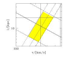
(a) NGC 5044

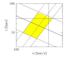
(b) NGC 1550

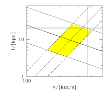
(c) M87

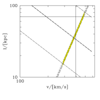
(d) AWM4

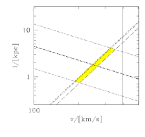
(e) Centaurus

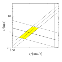
(f) AWM7

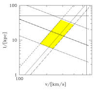
(g) A1795

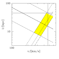
(h) Perseus

Figure 2: Range of the characteristic velocities $v$ and spatial scales $l$ of the gas motions which provide the necessary diffusion and dissipation rates. Along the thick dot-long dashed line the diffusion coefficient $D=C_{1}vl$ is constant and equal to the values listed in Table $3$, while the thin dot-long dashed lines show the effect of varying $C_{1}=0.11$ by factor of 1/3 and 3. Along the the dotted line the dissipation rate is equal to the cooling rate at $r_{0}=r_{cool}/2$; the dot-short dashed line is for $r_{0}=r_{cool}$ and the long dashed for $r_{0}=r_{cool}/4$ . At the intersection of these bands, two conditions are satisfied: i) the gas cooling is balanced by the dissipation and ii) the diffusion coefficient is of the right order. The vertical solid lines show the sound speed in the gas $c_{s}$ for $r=r_{cool}/2$ and half of it. In the plots where only one line is present, it corresponds to $c_{s}/2$.

Name	$r_{eff}/kpc$	$L_{TOT}/L_{\odot}^{B}$	$r_{a}/kpc$	$a(0)/a_{\odot}$	$b$	$r_{c}/kpc$	$\beta$	$n(0)10^{-3}/cm^{3}$
NGC 5044	$10.05$ [1]	$4.510^{10}$ [1]	$58.2$ [2]	$1.07$	$1.19$	$15$ [3]	$0.49$	$10.66$
NGC 1550	$9.1$ [4]	$3.510^{10}$ [5]	$0.8$ [4]	$0.95$	$0.14$	$2.5$ [4]	$0.35$	$7$
$M87^{*}$	$7.8$ [5]	$5.310^{10}$[21]	$20$ [7][8]	$0.85$	$0.38$	$2$ [6]	$0.42$	$130$
AWM4	$20$ [9]	$5.510^{10}$ [10]	$94$	$0.78$ [11]	$0.89$	$76$ [3]	$0.62$	$3.52$
$Centaurus^{*}$	$13$ [9]	$510^{10}$ [22]	$25$ [13]	$1.31$	$0.48$	$7.7$[14]	$0.57$	$165$
$AWM7^{*}$	$42$ [9] $16.6$ [12]	$1.410^{11}$ [15]	$7.2$ [16]	$1.6$	$0.3$	$3.5$ [17]	$0.25$	$165$
A1795	$34$[18]	$210^{11}$	$2.7$ [19]	$0.51$	$0.21$	$17$ [19][20]	$0.4$	$50$
Perseus	$15$	$1.610^{11}$	$48$	$0.54$	$0.18$	/	/	/

Table 2: Column (1) Name of the object (2)-(3) Effective radius and total blue luminosity of the central galaxy (4)-(5)-(6) Parameters of the iron abundance $\beta$-profile (7)-(8)-(9)Parameters of the gas density $\beta$-profile (see the text for the precise form). For the sources marked with ( $*$ ) the best fit was a double $\beta$-model; here we report the parameters of the dominant one. References:[1]Buote et al. 2004[2]Buote et al. 2003[3] Sanderson et al. 2003[4] Sun et al. 2003[5] de Vaucouleurs et al. 1991 [6] Matsushita et al. 2002[7] Matsushita et al. 2003[8] Gastaldello & Molendi 2002[9] Schombert 1987[10] Finoguenov et al. 2001[11] O’Sullivan et al. 2005[12] Bacon et al. 1985 [13] Fukazawa 1994[14] Ikebe et al. 1999[15] Peletier et al. 1990[16] Furusho et al. 2003[17] Neumann & Böhringer 1995[18] Schombert 1988[19] Tamura et al. 2001[20] Ettori et al. 2002 [21] Arnaud et al. 1992[22] Laine et al. 2003.

This approach of choosing $r_{0}=r_{cool}/2$ implies that the cooling rates used will not be drastically different from source to source (as it would happen if for instance one uses a fixed value of $r_{0}$ for all the objects in the sample). The resulting constraints are shown in Fig. $2$. The thick dot-dashed line shows the combinations of $v$ and $l$ which give the same diffusion coefficient, while the thin dot-dashed lines show the effect of varying $C_{1}$ by factor of 1/3 and 3. The effect of varying $C_{2}$ by factor of 1/3 and 3 was estimated in Rebusco et al. (2005). Along the the dotted line the dissipation rate is equal to the cooling rate at $r_{0}=r_{cool}/2$; the dot-short dashed line is for $r_{0}=r_{cool}$ and the long dashed for $r_{0}=r_{cool}/4$ . The intersection of the two bands gives the locus of the combinations of $l$ and $v$ such that on one hand the diffusion coefficient is approximately equal to the required value (Table $3$) and on the other hand the dissipation rate is approximately equal to the cooling rate at $r_{cool}/2$.

3.4.2 Turbulent mixing vs turbulent dissipation

Since cluster atmospheres are characterized by positive gradient of the specific entropy, stochastic motions should also lead to the heat flow into the central region (e.g. Dennis & Chandran, 2004). Following their work we estimate the rate of heating due to the turbulent transport of high-specific-entropy gas into low-specific-entropy regions:

$$\Gamma_{tt}=\nabla\cdot(D\rho T_{gas}\nabla e),$$ (7)

where $T_{gas}$ is the temperature and $e=C_{V}ln(c_{s}^{2}/\gamma\rho^{\gamma-1})$ is the specific entropy (adiabatic index $\gamma=5/3$, specific heat at constant volume $C_{V}=3k/2\>\>n_{H}/\rho$ ).

First we consider the case of a diffusion coefficient independent of the radius. A typical example of $\Gamma_{tt}$ radial dependence (NGC 5044), for the diffusion coefficients taken from Table 3, is shown in Fig. 3. While the heat flow is always towards the center, the volume heating rate $\Gamma_{tt}$ is positive inside a certain radius and it becomes negative (i.e. cooling) in the outer regions. This is of course an expected result - for constant diffusion coefficient the heat flux $r^{2}\>D\>\rho\>T_{gas}\frac{\partial e}{\partial r}\sim r\>\rho$ (see eq.7) and there is likely to be a radius near which this function is almost independent from the radius. As it is seen in Fig. 3 the turbulent transport (dotted line) calculated for $D=9\times 10^{28}$ cm² s^-1 is an important source of heat in the innermost 10 kpc, but $\Gamma{tt}$ quickly declines with the radius. Obviously the diffusion coefficient has to increase with the radius if the turbulent heat transport $\Gamma_{tt}$ balances the cooling over a broad range of radii. For comparison the heating rate due to the dissipation of turbulent motions $\Gamma_{diss}$ (for the parameters taken from Table 3) is shown by the dashed line in Fig. 3. Note that the rate of dissipation is a very strong function of $v$ and variations in $v$ by a factor of 2 (for a fixed diffusion coefficient $\propto l\times v$) cause variations of $\Gamma_{diss}$ by a factor of 16 (see Fig. 3).

Figure 3: NGC 5044: the solid line shows the cooling rate as a function of radius; the dotted line is the heating rate $\Gamma_{tt}$ evaluated for $D=9\times 10^{28}$cm² s^-1: the thin line corresponds to the part where $\Gamma_{tt}$ is positive, while the thick one is for $\Gamma_{tt}<0$. The remaining lines represent the dissipation heating rate $\Gamma_{diss}$ for the same $D$, but different velocity and length scales: $l=l_{ref}=11$ kpc and $v=v_{ref}=245$ km/s (short-dashed), $l=l_{ref}/1.8$ and $v=1.8\>v_{ref}$ (dot-dashed), $l=1.8\>l_{ref}$ and $v=v_{ref}/1.8$(dot-dashed). For the other sources, these plots show a similar qualitative behavior.

Chandran (2005) considered convective motions in the cluster cores driven by the cosmic rays injected by a central AGN. In his two-fluid (thermal-plasma and cosmic-ray) mixing-length theory approach, the characteristic length and velocity scales are functions of the radius. Assuming that the turbulent heat transport is the dominant source of heat we calculated the diffusion coefficient $D_{0}(r)$ (needed to balance heating and cooling at every radius) by integrating the equation $\Gamma_{tt}=\Gamma_{cool}$ over the radius. The resulting diffusion coefficient linearly increases with the radius and it reaches the value of $D=9\times 10^{28}$cm² s^-1 at $r\sim$ 5 kpc. Such radially dependent diffusion coefficient produces progressively more and more efficient mixing with increasing distance and it leads to an abundance profile which drops to $\sim$0.1 already at $\sim$10 kpc (see Fig. 4).

We next assumed that $\Gamma_{diss}\approx\Gamma_{cool}$ at every radius and we calculated the quantity $v^{3}/l$ as a function of the radius. We then considered several possibilities for the radial dependence of $v$ and $l$ and we derived the corresponding diffusion coefficients.

$$D_{1}(r)= c_{1}vl(r), v={\rm const}$$ (8)

$$D_{2}(r)= c_{1}v(r)l, l={\rm const}$$

$$D_{3}(r)= c_{1}v(r)l(r), l(r)=0.3r.$$

The choice of $l(r)\propto r$ for $D_{3}(r)$ is motivated by the work of Chandran (2005). For the first two models the constant $v$ and $l$ were fixed at the values taken from Table 3. The abundance profiles obtained by integrating equation $1$ using these diffusion coefficients are shown in Fig. 4. The case of $D_{2}(r)$ (i.e. constant length scale $l$ and variable velocity scale $v$) fits the observed profile the best, while the other versions of $D(r)$ yield profiles which strongly deviate from the observed one.

From these plots one can conclude that it is possible to construct a model with radially dependent velocity and length scales such that the abundance profiles are approximately reproduced and that the dissipation of turbulent motions compensates the gas cooling over a wide range of radii. In the simplest model of this type ($D_{2}(r)$ above) the length scale is independent of the radius and the velocity scale is a slowly decreasing function of the radius.

Figure 4: NGC 5044: in both plots the solid line represents the observed abundance profile from which the constant value $a_{b}=0.3a_{\odot}$ is subtracted. The dotted line is for $D=D_{0}(r)$, the short-dashed for $D=D_{1}(r)$, the long-dashed for $D=D_{2}(r)$ and the dotted-dashed for $D=D_{3}(r)$(see subsection $3.4.2$ for an explanation): they show the expected abundances obtained according to equation $1$, starting from a flat zero profile (left panel, $\tau_{age}=5$ Gyr) and starting from the present-day profile (right panel, after $4$ Gyr from now). For the other sources, these plots display a similar qualitative behavior.

4 Results and their discussion

In Table $3$ the estimated values of the diffusion coefficient $D$, the characteristic velocity $v$ and the spatial length scale $l$ are listed. The set of the parameters for the iron enrichment models (listed in Table $4$, described in the Subsection $3.3$) are chosen in order to get a reasonable approximation of the observed profiles (see Fig. 1): a factor of $3$ smaller (or larger) diffusion coefficients produce too peaked (or too shallow) abundance profiles, inconsistent with the data.

For each source we made a consistency check evaluating the characteristic value of the diffusion coefficient by comparing the half mass radius of the observed central excess and the excesses produced by ejection and diffusion in the model. For small diffusion coefficients the metal distribution should follow the light distribution of the central galaxy (i.e. have the same effective radius), while for the increasing diffusion coefficient the effective radius should also increase. The values derived this way were consistent with those given in Table 3.

We then used the observed abundance peaks in each object as initial conditions and we calculated the subsequent evolution of the abundance profiles by fixing $D$ at the value from Table 3. In each case 3 times smaller (or larger) diffusion coefficient causes a quick steepening (or flattening) of the abundance peaks on time scales of a Gyr, while for diffusion coefficients of the order of those listed in Table $3$ the evolution is very slow on these time scales.

Name	$r_{cool}/2$ kpc	$D$ cm2 s-1	$l$ kpc	$v$ km s-1	$v/c_{s}$
NGC 5044	$20$	$9\times 10^{28}$	$11$	$245$	$0.51$
NGC 1550	$30$	$1.2\times 10^{29}$	$17$	$219$	$0.35$
M87	$20$	$8\times 10^{28}$	$10$	$250$	$0.34$
AWM4	$70$	$4.5\times 10^{29}$	$35$	$378$	$0.45$
Centaurus	$25$	$2\times 10^{28}$	$2$	$250$	$0.30$
AWM7	$50$	$6\times 10^{27}$	$1$	$193$	$0.18$
A1795	$50$	$1.3\times 10^{29}$	$14$	$278$	$0.25$
Perseus	$45$	$2.4\times 10^{29}$	$17$	$410$	$0.44$

Table 3: Estimate of the turbulence parameters for each source in our sample: name (1), half the cooling radius (2), diffusion coefficient (3), length scale (4) and velocity (5-6) of the gas motion.

The diffusion coefficients listed in Table 3 are mostly of the order of $10^{29}$ cm² s^-1, apart from those obtained for AWM4, Centaurus and AWM7 (see next subsections). These values can be considered as an an upper limit on the effective diffusion coefficient set by the random gas motions, since other processes may contribute to spreading the metals through the ICM.

Note that our simple model predicts the abundance to be the highest in the center of the cluster. Thus the abundance ”hole” observed in several well studied clusters (e.g. Böhringer et al. 2001, Schmidt et al. 2002) contradicts this conclusion. Potentially there are several explanations of the abundance hole. The simplest one supposes that the spectral models used for the abundance determination are not adequate for the central region, where a complicated mixture of different phases is present (e.g. Buote 2000). The resonant scattering and the diffusion of the line photons to larger radii is another possible explanation (e.g. Gilfanov et al. 1987, Molendi et al. 1998). However the model advocated here assumes that the gas in the center is not at rest, but it is involved in complex pattern of motions, which should reduce the effective optical depth (e.g. Churazov et al. 2004). Velocities of order the of few hundred km/s should make most of the lines optically thin. Less straightforward interpretations of the abundance hole are also possible, but they are beyond the scope of this paper. Future high energy resolution observations with micro-calorimeters should be able to resolve this question.

The sizes of the turbulent eddies obtained in this work are of the order of $10$ kpc and the characteristic velocities of the order of few 100 km/s. In our model the velocity scale is determined from the combination of two quantities $D\sim vl$ and $\Gamma_{diss}\sim v^{3}/l$: $v\sim(D\>\Gamma_{diss})^{(1/4)}$. As a result the estimates of $v$ come out very similar for all the objects, while $l$ spans over a larger interval, compensating for all the peculiarities. We stress that these estimates have to be taken with caution, due to the simplicity of the model and the to uncertainties in the enrichment process.

4.1 AWM4

This object is not a cooling flow cluster, unlike the other objects in the sample. It does contain however a central bright galaxy (NGC 6051) which should enrich the ICM with metals in the same way as in cooling flow clusters. The enrichment will be even more efficient in AWM4 because the gas density is relatively small and even a modest amount of metals should produce a prominent abundance peak. As one can see from Table 3 the diffusion coefficient required to explain the lack of such abundance peak in AWM4 is larger than for any other objects in the sample. The length scale is also the largest in the sample. This can be easily understood since in this source a large value of the diffusion coefficient is needed along with a modest heating rate. As it is clear from eq.(5) and (6) this can be most naturally done by setting a large value of the gas motions spatial scale $l$.

If we would like to stay within the frames of our model then this is the object with the strongest level of gas mixing. There is a powerful radio source in NGC 6051 which clearly interacts with the ICM (e.g. O’Sullivan et al. 2005). It is not obvious however if the central AGN alone is responsible for the gas mixing and for the appearance of AWM4 as a non-cooling flow cluster. The alternative would be a recent merger followed by an intensive mixing of the ICM, but this case seems to be excluded by observations (O’Sullivan et al. 2005).

4.2 Centaurus

The Centaurus cluster has a central abundance peak which is difficult to reproduce with the enrichment model presented above. In order to produce such a large amount of iron in the central excess of this cluster, a long accumulation time (of the order of $10$ Gyr) and a high SNIa explosion rate are necessary (see Table 3). With these parameters we get a diffusion coefficient of $\sim 1.5\times 10^{28}$ cm² s^-1.

A previous estimate by Fabian et al. (2005) obtains that the diffusion coefficient in Centaurus is lower than $6\times 10^{28}$ cm² s^-1, consistently with our findings. Our result is also consistent (within the uncertainties of the profiles) with the value found by Graham et al. (2005). Since Graham et al. (2005) use higher blue luminosity for the central galaxy, their choice of enrichment parameters is less extreme than our. They also adopted higher value of the central abundance peak ($a_{0}\sim 2a_{\odot}$), derived from fitting the spectra with a cooling flow model, while our lower central abundance ($a_{0}\sim 1.3a_{\odot}$) is based on the two-temperature fits by Sanders & Fabian (2002). For their choice of parameters supersonic velocities are required to satisfy the equations (5) and (6). For lower luminosity (see Table 2), subsonic solutions are possible. However the results for Centaurus cluster remain quite controversial.

One plausible explanation of the extremely steep abundance gradient in Centaurus is the recent disturbance of the gas in the cluster core. ”Cold fronts” are observed in many clusters with cool cores (e.g. Markevitch et al. 2000). These features are believed to form when the gas sloshing in the potential well brings layers of gas with different entropies in close contact: in a similar fashion layers of gas with different abundances can form a transient feature characterized by a steep abundance gradient. In the frame of the model discussed here any steep abundance gradient translates into strong limits on the diffusion coefficient.

4.3 AWM7

Taking the results of our analysis at face value, this cluster does not require strong stochastic motions to match the observed and predicted abundance profiles. There is also no evidence for a strong radio source in it(e.g. Furusho et al. 2003). From this point of view it is tempting to conclude that AWM7 is now passively cooling and that the activity of the central AGN is only about to start (in another cooling time $\sim 7\times 10^{8}$ years). Then our estimate of the velocity and the length scale based on the assumption of a balance of the gas cooling would overestimate the combination $v^{3}/l$ and underestimate $l$. Note however that Furusho et al. (2003) reported an unusual substructure in the metal distribution in the AWM7 core, which is at odds with the assumption that gas motions are almost absent in this cluster. Given that in several clusters an abundance hole is observed it is possible that the substructure in AWM7 has a similar nature.

4.4 Radio bubbles and stochastic gas motions

Vazza et al. (2006) simulated non-cooling flow clusters, fin
ding that the energy due to turbulent bulk motions scales with the mass of the cluster: similar calculations had been done by Bryan & Norman (1998). In these simulations the turbulence is a result of the cluster formation, while in the core of CF clusters one can expect that the AGN is playing a dominant role in driving the turbulence: as a consequence the mass scaling of the two processes may be different.

Allen et al. (2006) found recently a tight correlation between the estimates of the Bondi accretion rate on to the central black hole and the jet power (estimated from the observed expanding bubbles) in X-ray luminous elliptical galaxies (similar calculations have been previously done by Di Matteo et al. 2001, Churazov et al. 2002 for M87 and by Taylor et al. 2006 for NGC 4696). At the same time the comparison of the jet powers and the cooling rates (e.g. Bîrzan et al. 2005) also shows a reasonable agreement. These results suggest that the amount of energy provided by jets (in the from of bubbles of relativistic plasma) is regulated by the gas properties in such a way that the gas cooling is approximately compensated. One can compare the rough estimates of the turbulence length scales (of the order of few - few tens kpc , see Table 3) with the observed sizes of radio bubbles in cluster cores (e.g. Dunn & Fabian 2004, Dunn, Fabian & Taylor 2005, Churazov et al. 2001). Broadly the numbers are of the same order. E.g. the observed radio bubbles sizes in M87 vary from $\sim 1$ to $\sim 10$ kpc (depending if one refers to the inner lobes or to the torus-like eastern or the outer southern cavities). In the Perseus, A1795 and Centaurus clusters the observed bubbles sizes also fall in the range few - few tens kpc. The characteristic velocities of the bubbles motions are of the order of $\sim 0.5c_{s}$ and they are also broadly consistent with the values listed in Table 3. From this point of view the observed bubbles seem to have all the necessary characteristics required to drive the gas motions needed to spread the metals.

5 Conclusions

We show that the iron abundance profiles observed in a small sample of nearby clusters and groups with cool core are consistent with the assumption that metals are spreading through the ICM with effective diffusion coefficients of the order of $10^{29}$cm² s^-1. This value does not show any obvious trend with the mass or the ICM temperature of the system.

For characteristic velocities of the order of $300$ km/s and length scales of the order of $10$ kpc, the dissipation of the gas motions would approximately balance the gas cooling. When observations are available, our estimates of the turbulent length scales are consistent with the observed buoyant bubbles size, pointing at the central supermassive black hole as the likely origin of the core gas motions.

Two objects in our sample require very different diffusion coefficients: for AWM7 very small level of gas mixing is needed, while for AWM4 the mixing has to be very intense. It is possible that these two objects hint to the intermittence of the gas mixing and that they represent two different episodes of the cluster evolution: AWM7 is only weakly disturbed now (but it will likely be disturbed soon by the onset of AGN activity), while AWM4 has been already mixed recently. O’Sullivan et al. 2005, using the analogy with M87 (where an abundance gradient is present in spite of clear signs of a radio jets interaction with the ICM) suggested that it is unlikely that AGN activity is responsible for the absence of the abundance peak in AWM4. One cannot however completely exclude the possibility that in the past there was a period of truly violent AGN activity in AWM4, which not only removed the central abundance peak, but also destroyed the whole cooling flow.

Name	$a_{b}/a_{\odot}$	$M_{Fe}/M_{\odot}\times 10^{8}$	$r_{m}/kpc$	$k$	$SR/SNU$	$t_{age}/Gyr$	$D/[cm^{2}/s]\times 10^{28}$
NGC 5044	$0.2$	$1.5$	$42$	$1.1$	$0.26$	$8$	$12.2^{*}$
	# $0.3$	$0.5$	$36$	$1.1$	$0.15$	$5$	$8.7$
	$0.4$	$0.8$	$31$	$2$	$0.06$	$8$	$9$
NGC 1550	# $0.3$	$0.8$	$67$	$1.1$	$0.15$	$7.6$	$12.6^{*}$
M87	# $0.2$	$0.9$	$46$	$1.1$	$0.15$	$6.2$	$8.3$
	$0.3$	$0.8$	$29$	$1.1$	$0.24$	$5$	$8.8$
AWM4	# $0.2$	$7.2$	$83$	$2$	$0.33$	$10$	$45$
	$0.3$	$3.8$	$64$	$1.1$	$0.34$	$10$	$37.5$
	$0.4$	$1.9$	$55$	$2$	$0.30$	$6.4$	$25^{*}$
Centaurus	# $0.3$	$6.0$	$47$	$2$	$0.33$	$10$	$2^{*}$
	$0.4$	$3.6$	$37$	$1.1$	$0.39$	$10$	$1^{*}$
AWM7	# $0.3$	$7.6$	$50$	$1.7$	$0.15$	$10$	$0.6^{*}$
	$0.4$	$3.4$	$32$	$1.1$	$0.15$	$8.7$	$0.5$
A1795	$0.2$	$16$	$140$	$2$	$0.30$	$8.4$	$36$
	# $0.3$	$2.9$	$62$	$1.1$	$0.15$	$5.4$	$12.5$

Table 4: Enrichment models:column (1) Name of the object (2) Total iron excess; the hash indicates the model that was used to produce the plots in Fig. 1 and 2 (3) Half mass radius (4) $k$ (5) Present-day SNIa rate (6) Source lifetime (For the definitions see the text)-(7) Effective diffusion coefficient: the models marked with the asterisk have an uncertainty due to the choice of the criterion to fix $D$ of a factor $\%/\times 2$, while for the other models the uncertainty is smaller.

References

- (1) Allen S. W., Fabian A. C., 1994, MNRAS, 269, 409
- (2) Allen S. W., Fabian A. C., Johnstone R. M., Arnaud K. A., Nulsen P. E. J., 2001, MNRAS, 322, 589
- (3) Allen A. W., Dunn R. J. H., Fabian A. C., Taylor G. B., Reynolds C. S., 2006, MNRAS (astro-ph/0602549)
- Anders & Grevesse, (1989) Anders E., Grevesse N., 1989, Geochimica et Cosmochimica Acta, 53, 197
- (5) Arnaud M., Rothenflug R., Boulade O., Vigroux L., Vangioni-Flam E., 1992, A&A, 254, 49
- (6) Bîrzan L., Rafferty D. A., McNamara B. R., Wise M. W., Nulsen P. E. J., 2004, ApJ, 607, 800
- (7) Bacon R., Monnet G., Simien F., 1985, A&A, 152, 315
- (8) Beuing J.,Döbereiner, Böhringer H., Bender R., 1999, MNRAS, 302, 209
- Böhringer et al. (2001) Böhringer, H., Belsole, E., Kennea, J., et al., 2001, A&A, 365, L18
- Böhringer et al. (2004) Böhringer H., Matsushita K., Churazov E., Finoguenov A., Ikebe Y., 2004, A&A, 416, 21
- BH (96) Briel U. G., Henry J. P., 1996, ApJ, 472, 131
- (12) Bryan G. L., Norman M. L., 1998, ApJ, 495, 80
- Betal (00) Buote D. A., 2000, MNRAS, 311, 176
- (14) Buote D. A., Lewis A. D., Brighenti F., Mathews W. G., 2003a, ApJ, 594, 741
- (15) Buote D. A., Lewis A. D., Brighenti F., Mathews W. G., 2003b, ApJ, 595, 151
- (16) Buote D. A., Brighenti F., Mathews W. G., 2004, ApJ, 607, L91
- Cappellaro, Evans, & Turatto (1999) Cappellaro E., Evans R., Turatto M., 1999, A&A, 351, 459
- (18) Chandran B.D.G., 2005, ApJ, 632, 809
- (19) Condon J. J. et al., 1998, AJ, 115, 1693
- (20) Churazov E., Forman W., Jones C., Böhringer H., 2000, A&A, 356, 788
- (21) Churazov E., Brüggen M., Kaiser C. R., Böhringer H., Forman W., 2001, ApJ, 554, 261
- Churazov et al. (2002) Churazov E., Sunyaev R., Forman W., Böhringer H., 2002, MNRAS, 332, 729
- Churazov et al. (2003) Churazov E.,Forman W., Jones C., Böhringer H., 2003, ApJ, 590, 225
- Churazov et al. (2004) Churazov E., Forman W., Jones C., Sunyaev R., Böhringer H., 2004, MNRAS, 347, 29
- Ciotti et al. (1991) Ciotti L.,D’Ercole A., Pellegrini S., Renzini A., 1991, ApJ 376 380
- Crawford et al. (2005) Crawford C. S., Hatch N. A., Fabian A. C., Sanders J. S., 2005, MNRAS, 363, 216
- Detal (94) David L. P., Jones C., Forman W., Daines S., 1994, ApJ, 428, 544
- De Grandi et al. (2004) De Grandi S., Ettori S., Longhetti M. Molendi S., 2004, A&A, 419, 7
- De Vaucouleurs et al. (1991) De Vaucouleurs G., De Vaucouleurs A., Corwin H. G., Buta R. J. Jr, Paturel G., Foqué P., 1991, Third Reference Catalogue of Bright Galaxies vol. II (Springer-Verlag)
- Dennis & Chandran, (2004) Dennis, T., Chandran, B., 2004, AAS, 36, 1592
- Dennis & Chandran, (2005) Dennis, T., Chandran, B., 2005, ApJ, 622, 205
- (32) Di Matteo T., Johnstone R. M., Allen S. W., Fabian A. C., 2001, ApJ, 550, L19
- Domainko et al. (2006) Domainko W. et al., 2006, A&A (astro-ph 0507605)
- (34) Dunn R.J.H., Fabian A.C., 2004, MNRAS, 355, 862
- (35) Dunn R. J. H., Fabian A. C., Taylor G. B., 2005, MNRAS, 364, 1343
- (36) Ettori S., Fabian A. C., Allen S. W., Johnstone R. M., 2002, MNRAS, 331, 635
- (37) Fabian A. C., Arnaud K. A., Bautz M. W., Tawara Y., 1994, ApJ, 436, L63
- (38) Fabian A. C. et al., 2000, MNRAS, 318, L65
- (39) Fabian A. C., Celotti A., Blundell K. M., Kassim N. E., Perley R. A., 2002, MNRAS, 331, 369
- Fabian et al. (2003) Fabian A. C., Sanders J. S., Allen S. W., Crawford C. S., Iwasawa K., Johnstone R. M., Schmidt R. W., Taylor G. B., 2003a, MNRAS, 344, L43
- (41) Fabian A. C. et al., 2003b, MNRAS, 344, L48
- (42) Fabian A. C., Sanders J. S., Taylor G. B., Allen S. W., 2005, MNRAS, 360, L20
- (43) Ferguson H. C., & Sandage A., 1990, AJ, 100, 1
- (44) Finoguenov A., David L. P., Ponman T. J., 2000, ApJ, 544, 188
- (45) Finoguenov A., Arnaud M., David L. P., 2001, ApJ, 555, 191
- Finoguenov et al. (2002) Finoguenov A., Matsushita K., Böhringer H., Ikebe Y., Arnaud M., 2002, A&A, 381, 21
- (47) Forman W. et al., 2005, ApJ, 635, 894
- (48) Fukazawa Y., 1994, PASJ, 46, L55
- Furusho, Yamasaki &Ohashi (2003) Furusho T., Yamasaki N.Y., Ohashi T., 2003, ApJ, 596, 181
- GM (02) Gastaldello F., Molendi S., 2002, ApJ, 572, 160
- (51) Gilfanov M. R., Sunyaev R.A., Churazov E., 1987, SvAL, 13, 3
- Getal (05) Graham J., Fabian A. C., Sanders J. S., Morris R. G., 2005, MNRAS (astro-ph/0602466)
- (53) hat05 Hatch N. A., Crawford C. S., Johnstone R. M., Fabian A. C., 2005, MNRAS (astro-ph/0512331)
- Hernquist (1990) Hernquist L., 1990, ApJ, 356, 359
- Ietal (99) Ikebe Y. et al., 1999, ApJ, 525, 581
- (56) Jerjen H., Dressler A., 1997, A&ASS, 124, 1
- Ketal (04) Kaastra J. S. et al., 2004, A&A, 413, 415
- (58) Kawaharada et al., 2003, PASJ, 55, 573
- (59) Koranyi D. M., Geller M. J., 2002, AJ, 123, 100
- Letal (03) Laine S. et al., 2003, AJ, 125, 478
- Mateal (97) Macchetto F. et al., 1997, ApJ, 489, 579
- (62) Markevitch M., Forman W., Sarazin C. L., Vikhlinin A., 1998, ApJ, 503, 77
- (63) Markevitch M., 2000, ApJ, 541, 542
- Metal (02) Matsushita K., Belsole E., Finoguenov A., Böhringer H., 2002, A&A, 386, 77
- Metal (03) Matsushita K., Finoguenov A., Böhringer H., 2003, A&A, 401, 443
- (66) Molendi S. et al., 1998, ApJ, 499, 608
- (67) Mushotzky, R. F., Loewenstein, M., 1997, ApJ, 481, L63
- Narayan & Medvedev (2001) Narayan R., Medvedev M. V., 2001, ApJ, 562, L129
- (69) Neumann M. et al., 1994, A&ASS 106, 303
- (70) Neumann D.M., Böhringer H., 1995, A&A, 301, 865
- Nevalainen et al. (2000) Nevalainen J., Markevitch M. & Forman W., 2000, ApJ, 532, 694
- (72) Oegerle W. R., Hill J. M., 1994, AJ, 107, 857
- (73) Owen F. N., Hardee P. E., Cornwell T. J., 1989, ApJ, 340, 698
- (74) Owen F. N., Eilek J. A., Kassim N E., 2000, ApJ, 543, 611
- (75) O’Sullivan E., Vrtilek J. M., Kempner J. C., David L. P., Houck J. C., 2005, MNRAS, 357, 1134
- (76) Peletier R. F., Davies R. L., Illingworth G. D., Davis L. E., Cawson M., 1990, AJ 100, 1091
- (77) Pedlar A. et al. 1990, MNRAS, 246, 477
- (78) Peres C. B. et al., 1998, MNRAS, 298, 416
- Peterson et al. (2003) Peterson J. R., Kahn S. M., Paerels F. B. S., Kaastra J. S., Tamura T., Bleeker J. A. M., Ferrigno C., Jernigan J. G., 2003, ApJ, 590, 207
- (80) Rebusco P., Churazov E., Böhringer H., Forman W., 2005, MNRAS, 359, 1041
- Renzini et al. (1993) Renzini A., Ciotti L., D’Ercole A., Pellegrini S., 1993,ApJ, 419, 52
- Sanders&Fabian (2002) Sanders J. S., Fabian A. C., 2002, MNRAS, 331, 273
- (83) Sanderson A. J. R., Ponman T. J., Finoguenov A., Lloyd-Davies E. J., Markevitch M., 2003, MNRAS, 340, 989
- Sanders et al. (2004) Sanders J. S., Fabian A. C., Allen S. W., Schmidt R. W., 2004, MNRAS, 349, 952
- (85) Sanderson A. J. R., Ponman T. J., Finoguenov A., Lloyd-Davies E. J., Markevitch M., 2003, MNRAS, 340, 989
- Schmidt et al. (2002) Schmidt R. W., Fabian A. C., Sanders J. S., 2002, MNRAS, 337, 71
- (87) Schombert J. M., 1987, ApJSS, 64, 643
- (88) Schombert J. M., 1988, ApJ, 328, 475
- (89) Schreier E. J., Gorenstein P., Feigelson E. D., 1982, ApJ, 261, 42
- (90) Sparks W. B., Biretta J. A., Macchetto F., 1996, ApJ, 473, 254
- (91) Sun M. et al., 2003, ApJ, 598, 250
- (92) Sutherland R. S., Dopita M. A., 1993, ApJS, 88, 253
- (93) Tamura T. et al., 2001, A&A, 365, L87
- (94) Takahashi I., Kawaharada M., Makishima K., Ikebe Y., Tamura T., 2003, Proceedings of The Riddle of Cooling Flows in Galaxies and Clusters of Galaxies, Ed. Reiprich,Kempner&Soker
- (95) Taylor G. B., Sanders J. S., Fabian A. C., Allen S. W., 2006, MNRAS, 365, 705
- (96) Tozzi P.,Rosati P., Ettori S., Borgani S., Mainieri V., Norman C., 2003, ApJ, 593,705
- (97) Vazza F., Tormen G., Cassano R., Brunetti G., Dolag K., 2006, accepted in MNRAS (astro-ph 0602247)
- Voigt & Fabian (2004) Voigt L. M., Fabian A. C., 2004, MNRAS, 347, 1130