The distribution of absorption in AGN detected in the XMM-Newton observations of the CDFS

Abstract

We have used very deep XMM-Newton observations of the Chandra Deep Field-South to examine the spectral properties of the faint active galactic nucleus (AGN) population. Crucially, redshift measurements are available for $84\%$ (259/309) of the XMM-Newton sample. We have calculated the absorption and intrinsic luminosities of the sample using an extensive Monte Carlo technique incorporating the specifics of the XMM-Newton observations. Twenty-three sources are found to have substantial absorption and intrinsic X-ray luminosities greater than $10^{44}$ erg s^-1, putting them in the “type-2” QSO regime. We compare the redshift, luminosity and absorption distributions of our sample to the predictions of a range of AGN population models. In contrast to recent findings from ultra-deep Chandra surveys, we find that there is little evidence that the absorption distribution is dependent on either redshift or intrinsic X-ray luminosity. The pattern of absorption in our sample is best reproduced by models in which $\sim 75\%$ of the AGN population is heavily absorbed at all luminosities and redshifts.

1 Introduction

Recent X-ray spectral studies using XMM-Newton and Chandra (Piconcelli et al., 2003; Civano et al., 2005; Mateos et al., 2005a) have begun to unravel the nature of the faint X-ray sources that make up the bulk of the extragalactic X-ray background (XRB) below 10 keV. Most of these sources are accretion powered AGN (Barger et al., 2003; Page et al., 2003). However, the population is far from homogeneous; the AGN exhibit a range of spectral properties, both in X-rays, and at other wavelengths. Unified models of AGN (e.g. Antonucci, 1993), have been reasonably successful in explaining the observational differences between the various classes of AGN/Seyfert galaxies. The X-ray spectra of the AGN can, in the majority of cases, be adequately described by a power-law model, in many cases with some degree of absorption. The AGN with significant X-ray absorption are predominantly identified with narrow emission line galaxies, and are seen as higher redshift, higher luminosity analogues of nearby Seyfert 2 galaxies. Population synthesis models such as those of Comastri et al. (1995), Gilli, Salvati & Hasinger (2001) and Ueda et al. (2003) use a superposition of faint AGN to reproduce the observed XRB. These models incorporate a large fraction of absorbed AGN in order to reproduce the hard spectrum of the XRB. Gilli, Salvati & Hasinger (2001) found that the XRB could be reproduced using a model in which the absorbed and unabsorbed AGN shared a common intrinsic X-ray luminosity function. A similar AGN population model was found to represent adequately the multi-wavelength properties of AGN in the GOODS dataset (Treister et al., 2004). In our previous work (Dwelly et al., 2005), we compared the X-ray colour distribution of sources detected in the $13^{H}~{}$ XMM-Newton deep field with the X-ray colour distributions predicted by a number of model $N_{H}$ distributions. We found that the best match to the data was made by a $N_{H}$ distribution model in which absorbed and unabsorbed AGN share the same intrinsic luminosity function, and where the number of AGN per unit $\log N_{H}$ is proportional to $(\log N_{H})^{8}$.

However, the results from other studies based upon deep X-ray surveys (e.g. Piconcelli et al. 2003; Ueda et al. 2003; Cowie et al. 2003; Barger et al. 2003, 2005), appear to contradict some of the foundations of these simple synthesis models. These studies all found that on average, the absorbed AGN which are optically identified lie at lower redshifts, and have lower intrinsic luminosities, than their unabsorbed counterparts.

Clearly the relationship between absorption and luminosity in the AGN population requires further examination. Therefore, in order to constrain the relationship between AGN luminosity, redshift and absorption we have undertaken a study of the X-ray properties of AGN in the Chandra Deep Field-South (CDFS). In this study we examine the 500 ks XMM-Newton European Photon Imaging Camera (EPIC) observations of the CDFS (hereafter XMM-CDFS) which provide a superb dataset for measuring the spectral properties of faint X-ray sources. The EPIC imaging reaches to fluxes well below the break in the 2–5 keV source counts, covers around 0.19 deg² and contains enough photons to permit broad band X-ray spectral analysis for even the faintest sources. The studies of Streblyanska et al. (2004) and Braito et al. (2005) have also used the XMM-CDFS dataset to investigate the X-ray spectra of a number of the brighter AGN in the field. However, until this work, there has been no investigation of the X-ray properties of the entire source population detected in the XMM-Newton imaging.

The EPIC data are complimented by Chandra observations (Giacconi et al., 2002; Lehmer et al., 2005), which provide sub-arcsecond positions for the majority of the EPIC sources, allowing us to identify uniquely the X-ray sources with optical counterparts. What is more, the entire EPIC field of view is covered by the COMBO-17 survey (Wolf et al., 2004), providing photometric redshift estimates for nearly all $R<24$ optical counterparts. We use an extensive Monte Carlo simulation process to recover the $N_{H}$ and intrinsic luminosity of the AGN detected in our sample. We also use the simulations to compare directly the distribution of sources with the predictions of a number of AGN population models.

This paper is laid out as follows. In section 2.1 we describe the reduction of the XMM-Newton data, and the source detection process. In section 3 we detail how we have correlated this with the other datasets available in the CDFS. In section 4 we introduce our Monte Carlo method for calculating the absorption and luminosity of the sample, and we demonstrate its fidelity. In section 5 we present the distribution of absorption, luminosity and redshift in the XMM-CDFS sample and compare it to the predictions of a number of AGN population models. Finally, in section 6 we compare our results to those found by other studies and discuss the implications for AGN population models.

Throughout the paper we use a lambda-dominated flat cosmology with $H_{0}=70$ km s^-1Mpc^-1, $(\Omega_{M},\Omega_{\Lambda})=(0.3,0.7)$. $S_{E_{a}-E_{b}}$ denotes the flux of a source in the observed $E_{a}$–$E_{b}$ keV band, corrected for Galactic absorption. $L_{2-10}$ refers to an object’s intrinsic X-ray luminosity (that is, before absorption), in the rest-frame 2–10 keV energy band. $N_{H}$ is the equivalent hydrogen column density in units of cm^-2.

2 Observations and data reduction

2.1 The XMM-Newton dataset

The XMM-Newton data consist of two observations carried out in July 2001, and six in January 2002. The observations all have similar pointing centres (approximately $RA=03^{h}32^{m}27^{s}$, $Dec=-27\degr 48\arcmin 55\arcsec$), but the Jan 2002 observations have position angle rotated $\sim 180\degr$ with respect to the July 2001 observations. The XMM-Newton data cover $\sim 0.19$ deg² (nearly twice the sky area of the 1Ms Chandra observations), and total around 500 ks. All three EPIC detectors (MOS1, MOS2 and pn) were operated with the ‘Thin1’ filters and were in full frame mode. The XMM-Newton data were reduced using standard Science Analysis Software (SAS, version 6.0) tasks, following the method described by Loaring et al. (2005). After temporally filtering periods of enhanced particle background from the event lists, we are left with approximately 340 ks of pn, and 395 ks of MOS exposure time. We notice an enhancement of the 0.2–0.5 keV background level for CCD #5 of MOS1, therefore we have discarded all the data from this chip in this energy range. We note that this effect has been reported recently by Pradas & Kerp (2005). We make an image, and an exposure map for each of the EPIC cameras, in each of the 0.2–0.5, 0.5–2, 2–5 and 5–10 keV energy bands, and for each of the eight observations. We also produce out-of-time event images for the pn camera in each of the four energy bands and for each observation which are used later by the background fitting algorithm. We have tied our coordinate system to the positions of (relatively) bright point-like X-ray sources detected in the 1Ms Chandra imaging of the field, taking into account the (-1.1″, 0.8″) offset between the Chandra positions and optical counterparts (Giacconi et al., 2002). A summary of the XMM-Newton observations is given in table 1.

Table 1: Summary of the XMM-Newton observations in the CDFS, showing the observation ID numbers, dates, exposure times, and telescope position angles (PA). Exposure times are given in kiloseconds for the pn and the average of the two MOS detectors, and indicate the length of good time remaining after removing periods of high background.

Observation	date	pn	MOS	PA
0108060401	2001-07-27	13.4 ks	20.2 ks	59°
0108060501	2001-07-28	31.7 ks	40.2 ks	59°
0108060601	2002-01-13	42.0 ks	47.6 ks	239°
0108060701	2002-01-14	67.9 ks	73.3 ks	239°
0108061801	2002-01-16	36.5 ks	54.8 ks	239°
0108061901	2002-01-17	38.9 ks	42.6 ks	239°
0108062101	2002-01-20	40.6 ks	43.3 ks	239°
0108062301	2002-01-23	69.3 ks	73.5 ks	239°
Total		340.3 ks	395.5 ks

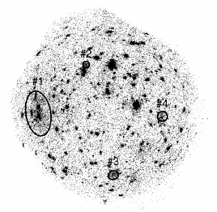
Figure 1: The combined XMM-Newton EPIC MOS+pn 0.5–2 keV image, background subtracted, and displayed on a linear scale. The field of view of EPIC is approximately 30′ in diameter. The four regions that we excluded due to the presence of extended emission are shown with numbered ellipses. These are likely to be galaxy clusters and are discussed in Appendix B.

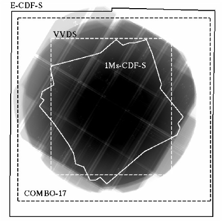
Figure 2: The combined XMM-Newton EPIC MOS+pn 0.5–2 keV exposure map. The peak pn-equivalent exposure time is $\sim 540ks$. We show the regions covered by the COMBO-17 survey (large black dashed rectangle), the 1Ms Chandra imaging (white polygon), and extended Chandra field (large black polygon), and the approximate area covered by the VVDS (smaller white dashed rectangle).

Visual inspection of the 0.2–0.5 and 0.5–2 keV images reveals four regions of large scale ($>1\arcmin$ diameter) diffuse emission, the locations of which are shown in figure 1. The most likely origin of this emission is from highly ionised gas in galaxy groups or clusters, the study of which is outside the scope of this AGN paper. The background fitting algorithm we have employed is not designed to remove diffuse emission on these scales. This unsubtracted diffuse emission will affect our measurement of the X-ray spectral properties of any AGN lying in these four regions, therefore we have excluded them from further analysis. The total sky area removed amounts to $\sim 28$ arcmin² (4% of the total XMM-Newton sky coverage).

We have used the iterative background fitting and multi-band source searching method to detect sources in the EPIC images. This process is described in detail by Loaring et al. (2005), but for completeness we give a summary here. Our method uses the SAS source searching routines EBOXDETECT and EMLDETECT, together with an iterative background fitting algorithm to detect sources simultaneously in the multi-band EPIC images. In order to maximise the sensitivity, the final source searching and source characterisation is carried out on composite images (one per energy band), summed over all observations and summed over all three EPIC detectors (MOS1, MOS2 and pn). In order to take account of the different effective areas, exposure times, and chip layouts/gaps of the EPIC detectors, we generate a composite exposure map. The contribution to this map from the MOS detectors was scaled according to the MOS/pn response ratio. The relative sensitivity of the MOS and pn detectors in each energy band was calculated with the XSPEC spectral fitting package (Arnaud, 1996) using standard on-axis EPIC pn and MOS response matrices. A similar process was used to determine the absolute pn count-rate to flux conversion factors in each energy band. For these calculations, we assume a power-law spectrum with photon-index 1.7, corrected for Galactic absorption of $8\times 10^{19}$ cm^-2, (Rosati et al., 2002). For the purposes of the final source detection process (in which an off-axis dependent PSF model is used), the position of the optical axis in the combined images is set to be the pn exposure-weighted mean of the pointings of the eight separate observations.

For each candidate detection, the source searching routine EMLDETECT reports a multi-band detection likelihood parameter, DET_ML, where $\textsc{DET\_ML}=-lnP$. $P$ is the probability (taking account of all four energy bands), that a random background fluctuation would occur within the detection element with an equal or greater number of source counts than the candidate detection. At the default minimum DET_ML level of 5.0, the “raw” EMLDETECT sourcelist contains 435 detections. It is not necessary for these sources to be individually detected in all four energy bands. At this low detection threshold, we expect a number of spurious detections to contaminate the faint end of the XMM-Newton sample; our method for dealing with these is discussed in the next section. A small number of the detections have very poorly determined positions ($\sigma_{pos}>5\arcsec$), or have poorly determined extent (the 90% error on the measurement of the extent is greater than the extent itself), and so we remove these from our sourcelist. We define three hardness ratios,

$$HR1 = \frac{R_{0.5-2}-R_{0.2-0.5}}{R_{0.5-2}+R_{0.2-0.5}}$$

$$HR2 = \frac{R_{2-5}-R_{0.5-2}}{R_{2-5}+R_{0.5-2}}$$ (1)

$$HR3 = \frac{R_{5-10}-R_{2-5}}{R_{5-10}+R_{2-5}}$$

where $R_{E_{a}-E_{b}}$ is the combined MOS+pn source count rate, corrected for vignetting, in the $E_{a}$ to $E_{b}$ (keV) energy band.

3 Matching to Chandra and optical catalogues

3.1 Cross correlation with Chandra observations of the field

The original 1Ms Chandra imaging of the CDFS covers the central part of the XMM-Newton field of view (FOV) to great depth (Giacconi et al., 2002; Alexander et al., 2003, see fig. 2). Recently, the Chandra sky coverage of the CDFS has been increased by a mosaic of four 250 ks Chandra pointings: the Extended Chandra Deep Field-South (E-CDFS) (Lehmer et al., 2005). We used the higher positional accuracy of the Chandra observations to aid unambiguous optical identification of the XMM-Newton sources. We matched the XMM-CDFS detections to sources in a combined Chandra catalogue constructed from the catalogues of Giacconi et al. (2002) and Lehmer et al. (2005). We have taken into account the (-1.1″, 0.8″) offset between the Chandra positions and optical counterparts in the Giacconi et al. (2002) catalogue. For those Chandra sources which appear in both the Giacconi et al. (2002) and Lehmer et al. (2005) catalogues, we mainly used the positions from the former. The point spread function of the XMM-Newton EPIC detectors is strongly off-axis angle dependent (Gondoin, 2000). At large off-axis angles the azimuthal component of the PSF becomes rather extended, whereas the radial component remains relatively constant. Therefore, we match the XMM-CDFS detections to Chandra counterparts using an ellipsoidal region. The semi-major axis of this ellipse is increased from 5″ for sources at the centre of the field, up to a maximum of 10″ for sources at off axis angles greater than 15′. The semi-minor axis is kept constant at 5″, and is oriented parallel to the line joining the source position and the nominal optical axis of the EPIC-pn detector. In addition, for the few XMM-CDFS detections which EMLDETECT determines to be slightly extended, we increase both semi-axes of the search ellipse by the measured extent. This choice of X-ray position matching criteria is discussed further in Appendix A.

Using these positional criteria, we find that 330 of the 431 XMM-CDFS detections are matched to Chandra sources; 185 of these matches are to sources in the 1Ms Chandra catalogue, and 145 are to sources in the E-CDFS catalogue. For the XMM-CDFS sources with no Chandra counterpart, we have manually examined the XMM-Newton and Chandra images. We find that in 15 cases, there is a nearby Chandra counterpart just outside the matching ellipse. We adopt the Chandra positions for these sources. Figure 3 shows the positional offsets between these matched XMM-CDFS and Chandra sources.

The determination of the XMM-Newton detection likelihood limit is a balance between the desire to include as many sources in our sample as possible, against the need to minimise the number of spurious detections. We could simply reject all XMM-Newton detections that are not matched to Chandra sources. However, whilst the headline flux limits achieved by the Chandra observations are fainter than those for the XMM-CDFS, the coverage is not uniform over the XMM-Newton FOV. What is more, the relative sensitivity of the XMM-Newton and Chandra detectors varies with energy. In particular, XMM-Newton EPIC is much more sensitive than Chandra at very high photon energies ($>5$ keV), and at very low photon energies ($<0.5$ keV), so sources having either very hard or very soft spectra will be preferentially detected with XMM-Newton. The XMM-Newton and Chandra observations of the CDFS span approximately four years, therefore intrinsic variability on timescales of several months to years could also account for sources appearing in some catalogues and not others. For these reasons, and because this study is based primarily upon XMM-Newton data, we curtail our XMM-CDFS sourcelist purely on the basis of the XMM-Newton detection likelihood. However, we set the level of this such that approximately $90\%$ of the XMM-Newton detections have Chandra counterparts. At a detection likelihood threshold of 8.5, we find that there are 335 XMM-Newton detections and 302 ($90.1\%$) of these have at least one Chandra counterpart.

There are 16 cases where a XMM-CDFS detection has more than one Chandra source inside (or very close to) the matching ellipse. In order to determine whether these are genuinely confused sources, we have manually inspected the XMM-Newton images, the 1Ms Chandra images (Alexander et al., 2003), and the E-CDFS images (Lehmer et al., 2005). In one case, the “confusion” appears to be the result of a single real astrophysical source appearing in both the 1Ms and E-CDFS Chandra catalogues. We chose the E-CDFS source in this case. We find that in the other cases, the XMM-Newton detection is matched to a clearly separated pair of Chandra sources. However, for four of these, there is a large brightness contrast between the two Chandra sources, and so we do not consider the XMM-CDFS source to be “confused”. We have removed from our sample the remaining eleven truly “confused” XMM-Newton detections because their XMM-Newton determined properties are superpositions of more than one real astrophysical source. The small number of detections that we have had to remove demonstrates that source confusion plays only a small role ($\sim 3\%$ of sources) in (high Galactic latitude) XMM-Newton surveys of several hundred kiloseconds.

Figure 3: Upper panel: The differences between the positions determined using XMM-Newton and Chandra as a function of XMM-Newton off-axis angle. The XMM-CDFS sources with Chandra counterparts are shown with circles for matches to Chandra 1Ms sources, and triangles for matches to E-CDFS sources. Those XMM-Newton sources manually matched to a Chandra source are highlighted with boxes. XMM-CDFS sources which do not have Chandra counterparts are shown with small square symbols at offset = -0.5.. The “confused” XMM-Newton detections are marked with crosses. Bottom panel: The differences between the X-ray position and the position of the optical counterpart, as a function of XMM-Newton 0.2–10 keV flux. The XMM-CDFS sources which have Chandra counterparts are shown with circles (1Ms matches) and triangles (E-CDFS matches), and those which do not have Chandra counterparts are shown with small square symbols. XMM-CDFS sources having no optical counterpart within the matching region are placed at offset =-0.5.

3.2 Optical counterparts and redshifts

The CDFS has been the target for a number of space and ground based deep optical/infrared imaging campaigns, which cover different parts of the field to different depths (e.g. Arnouts et al., 2001; Wolf et al., 2004; Giavalisco et al., 2004). A large amount of VLT-FORS time has been expended on optical spectroscopy of counterparts to X-ray sources detected in the 1Ms Chandra survey (Szokoly et al., 2004). Zheng et al. (2004) used these spectroscopic identifications together with optical and NIR measurements to estimate redshifts for virtually all of the X-ray sources in the 1Ms Chandra catalogue of Giacconi et al. (2002). Initially, we adopted the Zheng et al. (2004) estimates for all of the 167 XMM-CDFS detections matched to sources in the 1Ms Chandra catalogue. However, as noted by Barger et al. (2005), a number of the Zheng et al. (2004) optical counterparts have relatively large offsets from the X-ray source positions. We have manually examined the Chandra vs optical positions for the sources where the optical position stated by Zheng et al. (2004) is more than 2″ from the 1Ms Chandra position, or where there is more than one COMBO-17 source within 2″ of the 1Ms Chandra position. We have drawn upon the Chandra 1Ms images (Alexander et al., 2003), the E-CDFS images (Lehmer et al., 2005), the COMBO-17 optical images (Wolf et al., 2004), and the GEMS/GOODS ACS images (Caldwell et al., 2006), to choose the most likely optical counterparts. For sixteen cases (i.e. 10% of those sources that were examined), we decided that an alternative optical source was a more likely counterpart to the X-ray source. All of these alternative optical counterparts are closer to the X-ray position than the counterpart chosen by Zheng et al. (2004), and most are optically fainter. The ID numbers of these sources in Zheng et al. (2004) are 3, 17, 23, 25, 36, 61, 64, 70, 97, 99, 213, 517, 528, 548, 591 and 641. Where possible, (four cases) we have used the COMBO-17 redshift estimates for our preferred counterpart. Otherwise we consider the X-ray source to be optically unidentified. We note that for another six of the Zheng et al. (2004) sources, the correct spectroscopic redshift is quoted, but an incorrect optical position is stated. These were all cases where the X-ray sources had multiple optical counterparts listed in Szokoly et al. (2004).

We note that several of the XMM-CDFS detections matched to 1Ms Chandra sources have faint ($R>25$) optical counterparts for which photometric redshifts have been calculated by Mainieri et al. (2005b). However, in each case, the Mainieri et al. (2005b) redshift estimate is in agreement with the Zheng et al. (2004) value within the errors. So for simplicity and consistency, we prefer to adopt the Zheng et al. (2004) redshift estimate.

For the XMM-CDFS detections having a counterpart in the E-CDFS Chandra catalogue, and where an optical counterpart is found, we adopt the optical counterpart position from Lehmer et al. (2005). We use the COMBO-17 photometric redshift if there is an object in the COMBO-17 catalogue within 1″ of the optical position given by Lehmer et al. (2005). We find that in several cases, the optical counterpart has also been spectroscopically identified (i.e. it appears in the VVDS catalogue of Le Fevre et al. 2004, or the Szokoly et al. 2004 field galaxy list), and so for these XMM-CDFS sources we adopt the spectroscopic identifications.

For the 33 XMM-CDFS detections having no Chandra counterpart, we have attempted to assign an optical counterpart from the COMBO-17 catalogue. Our starting point was to choose the optically brightest source inside the variable matching ellipse discussed earlier. We then manually examined the X-ray and optical images to determine if this was the correct choice. For most of these sources, we adopted the initial choice of counterpart. However, for two sources, we chose an alternative optical counterpart because of a co-location with an enhancement in the E-CDFS image. For 13 of the XMM-CDFS sources without Chandra counterparts, the XMM-Newton detection is most likely due to diffuse emission from a group or cluster. That is, there are several galaxies having similar photometric redshifts located close to the XMM-Newton position. We have excluded these detections from our final XMM-CDFS sample, as they are unlikely to be AGN. There is one XMM-CDFS detection located away from the centre of a bright ($R\sim 17$) face-on spiral galaxy. The soft X-ray colours of this source, together with its non-detection by Chandra suggest that it is likely to be due to diffuse emission, and so we remove this detection from the sample. Finally, there were two XMM-CDFS sources located at the edge of the XMM-Newton FOV, outside the E-CDFS and COMBO-17 coverage. For simplicity, we have removed these two sources from our sample. The lower panel of figure 3 shows the X-ray-optical position differences for all the XMM-CDFS sources as a function of X-ray flux.

We note that the XMM-CDFS sample contains several low redshift sources with fluxes that imply very low luminosities ($L_{2-10}\sim 10^{40}$ erg s ${-1}$). It is therefore feasible that our sample contains a small number of ultra luminous X-ray (ULX) sources. Lehmer et al. (2006) have recently used Chandra deep field data to look for low X-ray luminosity sources lying off-axis in low redshift, optically bright galaxies. The Lehmer et al. (2006) sample contains 8 objects within the area covered by the XMM-Newton observations of the CDFS, but only one of these (J033234.73-275533.8 at $z=0.038$) is associated with an XMM-CDFS source. We exclude this object from our sample because it is unlikely to be an AGN.

In summary, after applying our XMM-Newton detection likelihood and positional criteria, and after removing the detections which are confused or unlikely to be point sources, there are 309 sources in the XMM-CDFS sample. Of these, 291 have Chandra counterparts, 278 are matched to optical counterparts, and 259 (84%) have optical spectroscopic identifications and/or photo-z estimates. Fifteen of these are associated with Galactic stars, and one with a candidate ULX in a low redshift galaxy. Figure 4 compares the optical magnitudes of the XMM-CDFS sources to their 0.2–10 keV X-ray flux. Note that over a third (109/309) of the XMM-CDFS sources are optically faint ($R>24$).

Figure 4: Distribution of 0.2–10 keV flux vs $R$ band optical counterpart magnitudes for the point like sources in the XMM-CDFS sample. Objects identified as Galactic stars are indicated with crosses. XMM-CDFS detections with Chandra counterparts are shown with small circles (1Ms matches), and small triangles (E-CDFS matches). XMM-CDFS detections without Chandra counterparts are shown with small boxes. XMM-CDFS detections with no optical counterpart, or a counterpart fainter than $R=26.5$ are marked with upward pointing arrows. Very optically bright counterparts are placed at $R=16$, and marked with downward facing arrows. Objects with no redshift estimate are highlighted with large circles. Optical magnitudes are taken from Wolf et al. (2004), Giacconi et al. (2002), and Lehmer et al. (2005). Dashed lines show several values of X-ray-to-optical flux ratio $S_{0.2-10}/S_{R}$, where the optical flux $S_{R}$ is calculated from the R-band magnitude: $S_{R}=10^{-5.5-0.4R}$ erg s^-1 cm${}^{-2}~{}$ (Barger et al., 2003).

4 Estimating the intrinsic properties of the sample using X-ray colours and Monte Carlo simulations

It has been shown by several authors (e.g. Mainieri et al., 2002; Della Ceca et al., 2004; Perola et al., 2004; Dwelly et al., 2005) that X-ray hardness ratios can be utilised to determine the spectral properties of faint XMM-Newton sources, and in particular, the amount of absorption. This approach relies on the observed source belonging to some assumed family of spectral types, for which the spectral parameters can be deduced. Spectral analyses of relatively bright AGN have shown that nearly all can be broadly described by a spectral model consisting of a primary power-law with slope $\Gamma\sim 1.9$, attenuated with some absorbing column of neutral material (e.g. Piconcelli et al., 2003; Page et al., 2006). A number of additional spectral model components are sometimes required to provide the best fits to the highest signal to noise AGN spectra, although these extra components are generally much less important than the primary power-law component when considering broad band X-ray colours. However, in our previous work (Dwelly et al., 2005), we found that we were able to provide a better match to the X-ray colours of AGN detected in the $13^{H}~{}$ deep XMM-Newton field by including an unabsorbed cold reflection component to the AGN spectral model; we use this as our baseline spectral model. The most important effect of the reflection component is to harden the spectrum at high energies ($E>5$ keV), and thus it reduces the amount of absorption needed to explain the X-ray spectrum of AGN with hard-sloped spectra.

The traditional approach to estimate the absorption in faint X-ray detected AGN, is to fit the observed multi-band X-ray hardness ratios to a model spectrum using a spectral fitting package such as XSPEC. However, there is a large degree of degeneracy in such an approach because of the number of fitted spectral parameters ($N_{H}$ and/or $\Gamma$), compared to the limited number of data points (it is typical for authors to use just a single hardness ratio measure between the 0.5–2 and 2–10 keV energy bands). We have devised a novel Monte Carlo approach, in which we deduce the intrinsic properties of sources in the XMM-CDFS sample by comparing them to the “output” properties of a library of simulated AGN. This method allows us to take account of the scatter of sources in multiple $HR$ space (which may be strongly asymmetric, and is dependent on the observations), and so allows a rigorous estimation of confidence intervals. What is more, we can use our simulation method to compare directly the source distributions predicted by various synthesis models, against those seen in our sample. We first summarise the method used to generate a simulated library of sources, and then describe the absorption and intrinsic luminosity estimation processes.

This approach allows us to treat all the identified sources in the XMM-CDFS sample in a consistent, uniform fashion, as opposed to examining the brighter sources using a different method to the fainter sources.

4.1 Monte Carlo simulations of the AGN populations

A detailed description of our Monte Carlo simulation process is given in Dwelly et al. (2005). Here we give a short summary. A population of AGN is randomly generated according to a model of the intrinsic X-ray luminosity function (XLF). To calculate the expected number of input AGN per field, the model XLF is integrated over the ranges $0.015<z<5.0$, and $10^{40}<L_{X}<10^{48}$ erg s^-1 (extrapolating from published models where necessary). For each of these AGN we assign a random redshift and luminosity, where the probability of a source having a particular value of $z$ and $L_{X}$ is taken from the XLF model. Each AGN is then randomly assigned values of $N_{H}$ and $\Gamma$ according to the respective model distributions. The $z$, $L_{X}$, $N_{H}$ and $\Gamma$ for each source are converted to multi-band XMM-Newton EPIC count-rates using the spectral model together with the EPIC response matrices. We adopt a spectral model consisting of a primary transmitted component and a component reflected from neutral material. The primary component is modelled as a power-law with an exponential cutoff ($E_{\mathrm{cutoff}}$ = 400 keV), absorbed by a neutral column of material. The reflection component is calculated from the pexrav model of Magdziarz & Zdziarski (1995), and we set the reflecting material to cover $\pi$ steradians, to be inclined at $30$ degrees to the viewing direction, and to have solar abundances.

We then simulate how this population would appear if it had been observed in the same manner as for the XMM-Newton observations of the CDFS. We generate simulated images separately for every combination of the four energy bands, three EPIC cameras, and eight observations, totalling 96 images per simulated field. These images incorporate the effects of the EPIC point spread function and detector response, use realistic exposure maps, and include a background at the same level as is observed in the real data. We sum these images over all observations and for the MOS1, MOS2 and pn cameras to produce one image per energy band. We mask out the four regions in the simulated images which are affected by diffuse emission in the real data. Background maps are calculated independently for each of the 96 images, (as for the real data) and then summed to produce one background map per energy band. We use the tasks EBOXDETECT and EMLDETECT to search the images for sources in the four energy bands simultaneously. The resultant output sourcelists are curtailed using the same detection likelihood and positional accuracy criteria as for the real XMM-Newton dataset.

We use the off-axis angle dependent matching ellipse described in section 3 to match output detections to input sources. To exclude output detections which are affected by confusion, we flag all output detections which are matched to two or more input sources having comparable (within a factor of five) full-band count-rates. This step mimics the method we used to find confused sources in the real XMM-CDFS sample.

4.2 Constructing the library of simulated sources

We have used the Monte Carlo method to generate a large reference library of simulated sources, and have used the following constituents to the AGN population model. We use the Luminosity Dependent Density Evolution (LDDE) XLF model of Ueda et al. (2003). The latter was fitted only over the $10^{41.5}\leq L_{2-10}\leq 10^{46.5}$ erg s^-1 range and to $z=3$. In order to cover the range of luminosities expected in the XMM-CDFS sample, we have extrapolated this XLF model down to $L_{2-10}=10^{40}$ erg s^-1, and out to $z=5$. We use a model $N_{H}$ distribution in which the number of AGN per unit $\log N_{H}$ is proportional to $(\log N_{H})^{8}$, and is independent of luminosity and redshift. To recreate the intrinsic scatter in the spectral slopes of AGN (Piconcelli et al., 2003; Page et al., 2006), we assign a randomly selected $\Gamma$ to each simulated source. These spectral slopes are randomly chosen from a Gaussian distribution centred on $\Gamma=1.9$, with $\sigma_{\Gamma}=0.2$, with the additional constraint that $1.2<\Gamma<2.6$. We adjusted the absolute normalisation of the model XLF such that the sky density of sources with 0.5–2 keV flux $\geq 2\times 10^{-15}$ erg s^-1 cm${}^{-2}~{}$ is similar to that measured in the XMM-CDFS sample (after removing confirmed non-AGN sources). A total of 2000 fields worth of simulations were carried out to generate the simulated source library; enough to ensure that redshift, luminosity and $HR$ space is well populated with simulated sources, but not so large as to consume a prohibitive amount of processing time. We have verified that this population model broadly reproduces the source counts of the extragalactic sources in the XMM-CDFS sample.

4.3 Models of the AGN $N_{H}$ distribution

During this study, we test the predictions of a number of model $N_{H}$ distributions, which are described below.

The “$(\log N_{H})^{\beta}$” $N_{H}$ distribution models: In these models the number of AGN with absorption $N_{H}$, per unit $\log N_{H}$, is proportional to $(\log N_{H})^{\beta}$, and is not dependent on redshift or luminosity. We have tested three variations by setting the parameter $\beta$ to 2, 5, and 8. A similar parameterisation of the $N_{H}$ distribution was introduced in the XRB synthesis models of Gandhi & Fabian (2003).

The “T04” $N_{H}$ distribution model: Treister et al. (2004), introduce an $N_{H}$ model in which the number of AGN having a particular value of absorption is based on a model in which the density of the obscuring torus decreases with distance away from its plane. The torus geometry in this model is independent of redshift and luminosity.

The “GSH01A” and “GSH01B” $N_{H}$ distribution models: Gilli, Salvati & Hasinger (2001) investigated the ability of two absorption distribution models to reproduce both the shape of the XRB and the AGN source counts below 10 keV. In both models, the distribution of $N_{H}$ within the absorbed AGN was taken to be the same as that observed in nearby Seyfert 2 galaxies (Risaliti, Maiolino & Salvati, 1999). In model “A”, the number ratio between AGN with $N_{H}\geq 10^{22}$ cm^-2 and those with $N_{H}<10^{22}$ cm^-2 is fixed to be 4. In model “B” the ratio increases with redshift; at $z=0$ the ratio is 4, and at $z\geq 1.32$ the ratio is 10.

The “U03” $N_{H}$ distribution model: Ueda et al. (2003) fitted a luminosity dependent model to the distribution of $N_{H}$ in their AGN sample. In this model, the fraction of AGN having $N_{H}>10^{22}$ cm^-2 decreases linearly with luminosity, from $\sim 0.6$ of AGN with $L_{2-10}\leq 10^{43.5}$ erg s^-1, to $\sim 0.4$ of AGN with $L_{2-10}=10^{45}$ erg s^-1.

4.4 Absorption estimation technique

The measured properties of the XMM-CDFS sources which we use to estimate the absorption are the redshift ($z$), the vignetting corrected count rate in the 0.2–10 keV band ($R_{0.2-10}$), and three hardness ratios ($HR1$, $HR2$, and $HR3$). The absorption and luminosity of each real source is estimated from those simulated library sources which have similar values of $z^{\prime}$, $R^{\prime}_{0.2-10}$, $HR1^{\prime}$, $HR2^{\prime}$, and $HR3^{\prime}$. The following process is carried out for each optically identified source in the XMM-CDFS sample.

We first select the objects from the simulated library which have similar redshift ($|z-z^{\prime}|\leq(1+z)\times 0.1$), a similar full band count-rate, $0.5<R^{\prime}_{0.2-10}/R_{0.2-10}<2$, and have similar hardness ratios to the real XMM-CDFS source ($|HR1-HR1^{\prime}|\leq 0.1$, $|HR2-HR2^{\prime}|\leq 0.1$, and $|HR3-HR3^{\prime}|\leq 0.2$). The weaker constraint on $HR3$ reflects the poorer counting statistics at harder energies. We compensate for the possible influence that the shape of the baseline $N_{H}$ distribution used to generate the simulated library may have on the estimation process. Statistical weights are calculated by counting, for a large number of bins in $N_{H}$, the numbers of library sources which satisfy the redshift and countrate criteria. The weight of each selected object is the inverse of the number counted in the $N_{H}$ bin in which it lies. A sliding box technique is then used to estimate the absorption in the real source from the $N_{H}$ values and weights of the selected objects. We choose the $N_{H}$ value where the sum of the statistical weight inside a sliding box of width 0.25 dex is maximised. The confidence interval is taken to be the range of $N_{H}$ about this peak which contains 68% of the statistical weight of the selected objects.

4.5 Intrinsic luminosity estimation technique

We estimate the intrinsic, rest-frame 2–10 keV luminosity ($L_{2-10}$) of the real sources using a similar technique as that used to estimate absorption. For each XMM-CDFS source, we select the subset of sources from the simulated library which have similar redshifts, count rates, and hardness ratios (using the same criteria as before). We can account for the differences between the $z,R_{0.2-10}$ of the real XMM-CDFS source, and the $z^{\prime},R^{\prime}_{0.2-10}$ of each of the selected library sources: the $L^{\prime}_{2-10}$ of the library sources are corrected by factors of $R_{0.2-10}/R^{\prime}_{0.2-10}$ and $d^{2}_{L}(z^{\prime})/d^{2}_{L}(z)$ (where $d_{L}$ is the luminosity distance). We then take the median of the corrected $L^{\prime}_{2-10}$ of the selected subset of simulated sources as our estimate of the intrinsic luminosity of the real source. The confidence interval is given by the range of corrected $L^{\prime}_{2-10}$ about the median value which contains 68% of the simulated subset.

4.6 Fidelity of the $N_{H}/L_{X}$ estimation technique

We have measured the efficacy of our absorption/luminosity estimation technique by quantifying both how well it is able to estimate the $N_{H}/L_{X}$ values of individual sources, as well as how well it can recover an $N_{H}/L_{X}$ distribution of a population of sources.

4.6.1 Ability to recover $N_{H}/L_{X}$ of individual sources

We constructed a test population of simulated AGN using the method described in 4.2. The equivalent of one hundred XMM-CDFS fields were generated. For each test source, we made an estimate of absorption and intrinsic luminosity using our $N_{H}/L_{X}$ estimation technique, in the same way as we would for the real sources. The estimated $N_{H}/L_{X}$ values for each test source are then compared to the input parameter values.

Figure 5: An illustration of the fidelity of our absorption estimation technique evaluated from a population of simulated test sources. The panels show the degree of scatter of output $N_{H}$ about input $N_{H}$ values for test sources in four redshift bins. The bold curves show the median input $N_{H}$ as a function of output $N_{H}$. The thin curves show the degree of scatter (they contain 68% of the test sources). The vertical lines show the lowest output $N_{H}$ value for which this scatter is less than $\pm 0.5$ dex in each redshift bin.

Figure 5 shows the relationship between the estimated and input $N_{H}$ for test sources in a number of redshift ranges. The technique recovers the input $N_{H}$ values very well for test sources having moderate to heavy absorption. However, for low absorbing columns, the scatter increases rapidly. This becomes increasingly apparent at higher redshifts, as more and more of the absorption is shifted out of the EPIC bandpass. We have calculated the level below which less than 68% of test sources have $N_{H}$ estimates within 0.5 dex of the input value. This ranges from $10^{21.1}$ cm^-2 for sources in the $0<z<0.5$ redshift range, up to $10^{22.6}$ cm^-2 for the $3<z<4$ range.

The estimation technique becomes less accurate at very high levels of absorption. This is not unexpected; for all but the highest redshift AGN having this level of absorption, virtually all the flux has been removed below 5 keV. Thus $HR1$ and $HR2$ contain little information, meaning that we have less diagnostic power to determine the amount of absorption. What is more, at these high column densities, the effects of Compton scattering, which are not included in our spectral model, will become significant in the spectra of the real sources. We are therefore cautious about the exact $N_{H}$ for any sources estimated to have an absorbing column of greater than $10^{24}$ cm^-2, but we can be confident that such objects are very heavily absorbed. However, because of X-ray selection effects, we expect our sample to contain rather few of these very heavily absorbed AGN.

Figure 6: An illustration of the fidelity of the intrinsic luminosity estimation technique, showing the difference between the estimated and input intrinsic luminosities of the test sources as a function of their estimated intrinsic luminosity. The lines show the median input luminosity and the levels which contain 68% of the test sources as a function of estimated intrinsic luminosity. The upper panel is for test sources with $N_{H}<10^{22}$ cm^-2, and the lower panel for test sources with $N_{H}>10^{22}$ cm^-2.

In figure 6 we show the relationship between estimated and input intrinsic luminosity for the test sources. The high fidelity of the technique is evidenced by the low scatter of points about the one-to-one relation (less than $\pm 0.2$ dex for most of the luminosity range).

4.6.2 Ability to recover $N_{H}/L_{X}$ distributions of a population of sources

We have investigated how well the estimation technique can recover an input model absorption distribution. In addition, we have checked that the initial choice of AGN population model used to generate the simulated source library does not have a major effect on the estimated $N_{H}/L_{X}$ distributions.

Figure 7: The ability of the $N_{H}$ estimation process to recover a the distribution of $N_{H}$ in a population of test sources. We show three test populations generated according to the XLF model of Ueda et al. (2003). The upper panel shows the $(\log N_{H})^{5}$ model $N_{H}$ distribution, the centre panel shows the T04 $N_{H}$ distribution, and the bottom panel shows the luminosity dependent U03 $N_{H}$ distribution. In each panel, the dot-dash solid line shows the shape of the input $N_{H}$ model The dotted line is the distribution of $N_{H}$ in the test sources output from the Monte Carlo simulations. The solid line is the distribution of $N_{H}$ which is recovered by applying our $N_{H}$ estimation technique to these output test sources.

We extend the method of section 4.6.1 to generate several simulated test populations, each of which is based upon a different input $N_{H}$ model. The $N_{H}$ distribution of each population is then recovered using our $N_{H}$ estimation technique. Figure 7 shows a comparison of the input and recovered absorption distributions for three different input $N_{H}$ models. We show the input distribution of absorption in the test model, as well as the distribution in the sources that are output by the Monte Carlo simulation process. Heavily absorbed sources are less likely to be detected by the XMM-Newton observations than sources with lower absorbing columns, this selection effect results in the differences between the input and output distributions (see section 4.7). Above column densities of $\sim 10^{21}$ cm^-2, the distribution of absorption recovered by our $N_{H}$ estimation method is a good approximation to the “true” $N_{H}$ distribution in the output test population. There are disparities at low absorbing columns, where the estimation method can provide only weak constraints on the $N_{H}$ values of the test sources. However, the total number of output test sources having estimated $N_{H}\leq 10^{21}$ cm^-2 is consistent with the total number having “true” $N_{H}\leq 10^{21}$ cm^-2.

Figure 8: Plots demonstrating the independence of our $N_{H}/L_{X}$ estimation technique from the X-ray luminosity function model used to generate the simulated source library. In the top panel, the solid line shows the distribution of “true” $N_{H}$ for a population of test sources, in this case generated using the $(\log N_{H})^{8}$ model together with the model XLF of Ueda et al. (2003). The dotted line is the $N_{H}$ distribution estimated when we use the simulated source library generated from the model XLF of Ueda et al. (2003). The dot-dash line shows the estimated distribution when we use a second source library which was generated from the “LDDE1” model XLF of Miyaji et al. (2000). The lower panel shows the equivalent plot for the input and estimated distributions of intrinsic luminosity.

We have investigated whether the luminosity function used to construct the simulated source library has an effect on the outputs of our $N_{H}/L_{X}$ estimation process. We first generated a test population of AGN distributed in redshift/luminosity space according to the XLF model of Ueda et al. (2003), and with an absorption distribution following the $(\log N_{H})^{8}$ model. We then used our $N_{H}/L_{X}$ estimation technique to recover the absorption and luminosity of these test sources. This was carried out twice, firstly using the original simulated source library (generated according to the model XLF of Ueda et al. 2003), and secondly using a new simulated source library in which the sources are distributed according to the “LDDE1” XLF of Miyaji, Hasinger & Schmidt (2000). Note that the “LDDE1” XLF model is defined in the observed 0.5–2 keV band, with no correction of luminosities for absorption. For the purposes of this study we convert the 0.5–2 keV observed frame luminosities of the Miyaji et al. (2000) model to rest frame 2–10 keV luminosities assuming a mean power law spectrum with slope $\Gamma=1.9$. This conversion does assume that the Miyaji et al. (2000) sample is predominantly AGN unabsorbed in the X-rays (see section 3.1 of Miyaji et al. 2000). Figure 8 shows the resultant $N_{H}$ and $L_{X}$ distributions recovered using the two different source libraries. The differences between the recovered $N_{H}$ distributions are relatively small: for accurately measurable absorbing columns ($10^{21.5}<N_{H}<10^{24.5}$ cm^-2) they agree to better than 10%. We compare this to the Poisson noise of $\geq 15\%$ in the 0.5 dex wide bins of $N_{H}$ measured in the XMM-CDFS sample. We conclude therefore that our $N_{H}$ estimation technique is not strongly dependent on the AGN population model chosen to generate the simulated source library. However, we note that for $L_{2-10}>10^{44}$ erg s^-1, there is a significant difference between the luminosity distributions recovered by the two simulated source libraries (which have markedly different redshift/luminosity distributions). In order to mitigate this effect, when applying our estimation technique to the real XMM-CDFS sample, we should use a simulated source library in which the sources have a broadly similar luminosity and redshift distribution to the sources in the sample. Therefore, for the remainder of this study, we have used a simulated source library that is generated according to the model XLF of Ueda et al. (2003), as described in section 4.2.

Figure 9: The X-ray completeness of the XMM-Newton observations as a function of absorption, intrinsic luminosity, and redshift. The contours are the boundaries of the regions where at least 50% of the input test population is detected in the simulated images. Left panel: The 50% completeness limits as a function of luminosity and absorption, for a number of redshift bins. Centre panel: The 50% completeness limits as a function of redshift and absorption, for a number of luminosity bins. Right panel: The 50% completeness limits as a function of redshift and luminosity, for a number of absorption bins. In each panel, the arrow serves as a guide to the eye, and indicates the direction of increasing X-ray completeness.

4.7 X-ray completeness of the XMM-CDFS sample

The probability that an AGN in the CDFS will be detected in the XMM-Newton observations depends on the object’s redshift, luminosity, absorption, and position in the FOV. In order to quantify the selection function in the XMM-CDFS sample, we have compared the input and output sources in a large simulated population generated using our Monte Carlo process. The X-ray completeness is simply the ratio of the number of output detections to the number of input sources, and is calculated for a number of bins in redshift, luminosity and absorption. Figure 9 shows the regions in luminosity, absorption, and redshift space where at least half of the input sources have output detections. The XMM-CDFS observations are capable of detecting at least half the members of any population of luminous ($L_{2-10}\geq 10^{44}$ erg s^-1) obscured QSOs at $z\sim 2$ even if they are absorbed with large column densities ($N_{H}\sim 10^{23}$ cm^-2).

4.8 Direct comparison of the sample with model AGN populations

We wish to compare directly the $N_{H},L_{X},z$ distribution observed in the XMM-CDFS sample with the distributions predicted by various AGN population models. To accomplish this we have used our Monte Carlo process to simulate a number of model AGN populations, then have applied our $N_{H}/L_{X}$ estimation technique to recover the $N_{H}/L_{X}$ distributions of the model populations. In this way we incorporate both the complex X-ray selection effects of the XMM-Newton observations, and account for the limitations of the $N_{H}/L_{X}$ estimation technique. Therefore, the output simulated source distributions from this process can be compared like-with-like to the real XMM-CDFS sample. We have compared the XMM-CDFS sample with the predictions made by the seven different $N_{H}$ model distributions described in section 4.3.

Simulated populations are generated for each of these $N_{H}$ models, according to both the LDDE XLF model of Ueda et al. (2003) as well as the “LDDE1” XLF model of Miyaji et al. (2000). As before, the XLF models are extrapolated to low luminosities ($L_{2-10}=10^{40}$ erg s^-1), and high redshifts ($z=5$). For each of the fourteen combinations of $N_{H}$ model and XLF model, the absolute normalisation of the XLF is adjusted in order that the simulated integral 0.5–2 keV source counts above $2\times 10^{-15}$ erg s^-1 cm${}^{-2}~{}$ match the integral source counts in the extragalactic XMM-CDFS sample. We simulate 100 fields worth of sources for each combination of $N_{H}$ model and XLF model. Finally, we apply the $N_{H}/L_{X}$ estimation process to recover the absorption and luminosity distributions of the simulated output populations.

5 Results

5.1 Applying the $N_{H}/L_{X}$ estimation technique to the XMM-CDFS sample

We find that our technique is able to evaluate the absorption and luminosity in the vast majority of the optically identified extragalactic sources in the XMM-CDFS sample. However, we find that because of their very soft spectra, two AGN are not matched to any objects in the simulated source library. We discuss the properties of these sources in Appendix C. There is one XMM-CDFS source which we find to have a 2–10 keV luminosity less than $10^{40}$ erg s^-1. For the purposes of all the comparisons made in this section, we have excluded this source because it lies outside the luminosity range simulated in the model AGN populations.

5.2 Source counts in the XMM-CDFS

In figure 10 we show the differential 0.5–2.0 keV source counts for the extragalactic (including unidentified) sources in the XMM-CDFS sample, and compare them to the predictions of several simulated model AGN populations. The shape of the predicted source count curves is dependent predominantly on the form of the XLF model rather than on the $N_{H}$ distribution. We see that the XLF model of Miyaji et al. (2000) predicts a 0.5–2 keV source count distribution which is rather steeper than that found in the XMM-CDFS. At 0.5–2 keV fluxes above $10^{-15}$ erg s^-1 cm${}^{-2}~{}$, the source counts predicted by the Ueda et al. (2003) XLF model are a good match to the shape of the source counts in the XMM-CDFS sample. However, the Ueda et al. (2003) XLF model under-predicts the observed numbers of sources at fainter fluxes. A Kolmogorov–Smirnov comparison of the predicted 0.5–2 keV source count distributions with the observed XMM-CDFS distribution finds that though the Ueda et al. (2003) XLF is favoured ($P_{KS}=0.3$), the Miyaji et al. (2000) XLF model cannot be completely rejected ($P_{KS}=0.06$). We remind the reader that for each model of the AGN population, the XLF normalisation has been adjusted such that the integral source counts in the simulated population match the 0.5-2 keV extragalactic source counts measured in the XMM-CDFS sample. (see section 4.8).

Figure 10: The differential source counts for the extragalactic XMM-CDFS sample as a function of flux in the 0.5–2 keV energy band. For comparison, we show the source counts predicted by several different simulated model AGN populations. The two dashed curves show the predictions when we combine the $(\log N_{H})^{8}$ model firstly with the XLF model of Ueda et al. (2003), and secondly with the “LDDE1” XLF model of Miyaji et al. (2000). The predicted source counts from model populations generated according to the GSH01A $N_{H}$ model are also shown (dot-dashed curves). At faint fluxes, the distributions are dominated by sources which have their strongest detections in the other energy bands.

5.3 The redshift and luminosity distributions in the XMM-CDFS sample

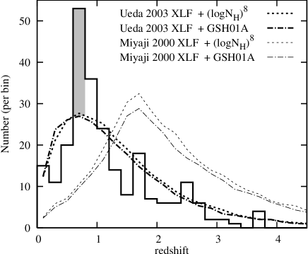
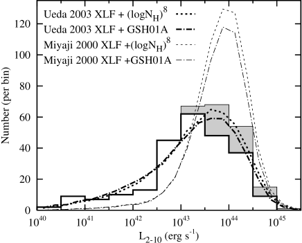
Figure 11: Distribution of redshifts (upper panel) and intrinsic 2–10 keV luminosities (lower panel) of identified extragalactic sources in the XMM-CDFS sample (solid histogram). For comparison, we show the distributions predicted by coupling the XLF model of Ueda et al. (2003) with the $(\log N_{H})^{8}$ and GSH01A $N_{H}$ distribution models (dashed and dot-dashed thick curves respectively). The thin curves show the rather different predictions made by combining the same $N_{H}$ distributions with the “LDDE1” XLF model of Miyaji et al. (2000). There are two large-scale structures identified in the CDFS at $z=0.67$ and $0.73$ (Gilli et al., 2003). At least 26 sources in the XMM-CDFS sample lie at these redshifts, as indicated by the shaded area in the upper panel. The shaded area in the lower plot shows the luminosity distribution of the 50 optically unidentified sources in the XMM-CDFS sample if they are assumed to lie at $z=2$.

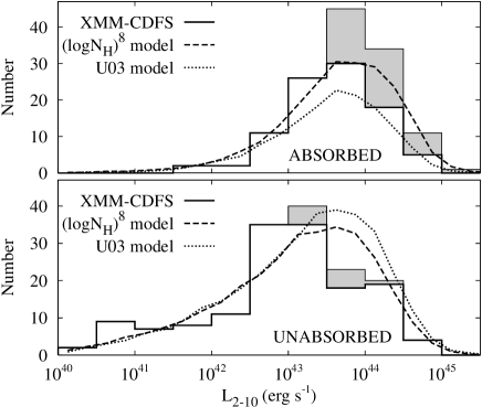
Figure 12: Similar to fig.11, but with the AGN divided into “absorbed” and “unabsorbed” objects. Here we set the threshold for an AGN to be considered “absorbed” to be $10^{22}$ cm^-2 for sources at $z<3$, and $10^{22.6}$ cm^-2 for sources at $z>3$. In each panel the solid histogram shows the XMM-CDFS sources, and the curves show the distributions predicted by coupling the XLF model of Ueda et al. (2003) with the $(\log N_{H})^{8}$ and U03 $N_{H}$ distribution models. The shaded areas in the lower two panels show the luminosity distribution of the optically unidentified sources in the XMM-CDFS sample if they are assumed to lie at $z=2$.

Figure 11 shows the redshift distribution of the optically identified XMM-CDFS sample compared with the redshift distributions for several of the simulated model populations. For clarity, we have shown only the results for the $(\log N_{H})^{8}$ and GSH01A models, because rather similar distributions are found in the other $N_{H}$ models. It is clear that the redshift distribution predicted by the XLF of Ueda et al. (2003) is a far closer match to the redshift distribution of the XMM-CDFS sample than the prediction from the XLF model of Miyaji et al. (2000). Figure 11 shows that the same holds true for the luminosity distribution. We remind the reader that the Miyaji et al. (2000) luminosity function is defined in the observed 0.5–2 keV band, and that we have converted to intrinsic rest frame 2–10 keV luminosities assuming an unabsorbed AGN X-ray spectrum (a $\Gamma=1.9$ powerlaw). This is of course a simplification; some of the AGN in the Miyaji et al. (2000) sample may be X-ray absorbed (and hence have hard spectra), and some of the AGN may have very soft X-ray spectra. But this scatter of slopes is unlikely to be a significant issue, and certainly not sufficient to explain the large differences between the redshift and luminosity distributions predicted by the Miyaji et al. (2000) XLF model and those seen in the XMM-CDFS sample.

In figure 12 we show redshift and luminosity distributions separately for the absorbed and unabsorbed AGN in the XMM-CDFS sample, and compare these to the predictions of the $(\log N_{H})^{8}$ and U03 $N_{H}$ models.

5.4 The $N_{H}$ distribution in the XMM-CDFS sample

In figure 13 we show the distribution of absorption in the optically identified sources in the XMM-CDFS sample determined using our $N_{H}$ estimation technique. The measured distribution is compared to the predicted distributions from the seven simulated $N_{H}$ models.

The high fidelity of our $N_{H}$ estimation process means that the recovered absorption distribution in the XMM-CDFS sample contains more information than just the relative numbers of absorbed and unabsorbed AGN; we can compare the shape of the absorption distribution measured in the XMM-CDFS sample with the shapes of the distributions predicted by the simulated model AGN populations. We have used the Kolmogorov–Smirnov (KS) test to make this comparison, the results of which are shown in table 3. This test clearly discriminates between the models, with the T04 $N_{H}$ distribution being the most strongly rejected.

Figure 13: The distribution of absorption in the optically identified XMM-CDFS sample (histogram) in comparison to the predicted distributions from the seven $N_{H}$ models (curves). The model $N_{H}$ distributions are for simulated populations generated according to the XLF model of Ueda et al. (2003). The shaded area shows the $N_{H}$ distribution of the optically unidentified sources if they are assumed to lie at $z=2$. For clarity, the model distributions are displayed in two groups.

5.5 The absorbed fraction in the XMM-CDFS and its dependence on luminosity and redshift

Figure 14: The fraction of XMM-CDFS sources with significant absorption, as a function of intrinsic 2–10 keV luminosity (upper panel), and redshift (lower panel). We set the threshold for a source to be considered “absorbed” to be $10^{22}$ cm^-2 for sources at $z<3$, and $10^{22.6}$ cm^-2 for sources at $z>3$. Error bars show the result for the XMM-CDFS sample: horizontal bars show the range over which the absorbed fraction has been calculated, and the vertical error-bars show the binomial error estimates, $\sqrt{f_{abs}(1-f_{abs})/N}$, where $f_{abs}$ is the absorbed fraction, and $N$ is the number of objects in the bin. The total numbers of XMM-CDFS sources in each bin are indicated on the plot. The curves show the absorbed fractions predicted by the $N_{H}$ distribution models, calculated in bins of width 0.5 dex in luminosity (upper panel), and width 0.5 in redshift (lower panel). In the upper panel, we also show the absorbed fraction in the XMM-CDFS sample if all unidentified sources are placed at $z=2$ (triangles).

In order to characterise the degree of luminosity and/or redshift dependence of the absorption distribution, we have examined the relative numbers of absorbed and unabsorbed AGN in the XMM-CDFS sample, and compared it to the predictions of the simulated model populations. We set the threshold for a source to be considered “absorbed” to be $10^{22}$ cm^-2 for sources at $z<3$, and to be $10^{22.6}$ cm^-2 for sources at $z>3$. When we tested the reliability of the $N_{H}$ estimation technique (see section 4.6.1), we found that for sources in the $3<z<4$ range, $10^{22.6}$ cm^-2 was the lowest level of absorption for which the scatter of output $N_{H}$ about input $N_{H}$ was less than 0.5 dex. The total absorbed fraction in the identified XMM-CDFS sample is $0.39\pm 0.03$, if the unidentified XMM-CDFS sources are assumed to lie at z=2, then the absorbed fraction becomes $0.45\pm 0.03$. These respective values can be considered as lower and upper bounds on the “true” total absorbed fraction. For comparison, in table 2 we show the total absorbed fractions predicted by each of the population models. When combined with the XLF model of Ueda et al. (2003), the $(\log N_{H})^{8}$,T04, and GSH01A $N_{H}$ models predict absorbed fractions consistent with these bounds. For each $N_{H}$ model, the populations generated using the Miyaji et al. (2000) XLF have a slightly higher absorbed fraction than for the Ueda et al. (2003) XLF. This is because the former XLF model predicts more objects at high redshifts (see fig. 11), where heavily absorbed AGN are selected against less strongly.

Table 2: The absorbed fraction predicted using the AGN population models for the XMM-CDFS sample. Predictions are shown for AGN populations generated according to each of the seven $N_{H}$ models tested in this study, using the Ueda et al. (2003) XLF model and the Miyaji et al. (2000) LDDE1 XLF model. The total absorbed fraction in the optically identified XMM-CDFS sample is $0.39\pm 0.03$. If the optically unidentified XMM-CDFS sources are assumed to lie at $z=2$, this fraction becomes $0.45\pm 0.03$.

$N_{H}$ model	XLF model
	Ueda et al. (2003)	Miyaji et al. (2000)
$(\log N_{H})^{2}$	0.283	0.297
$(\log N_{H})^{5}$	0.335	0.362
$(\log N_{H})^{8}$	0.409	0.422
T04	0.460	0.468
GSH01A	0.364	0.395
GSH01B	0.492	0.535
U03	0.301	0.311

Figure 14 shows the absorbed fraction as a function of both redshift and intrinsic luminosity compared to the distributions predicted from the Monte Carlo simulations of the $N_{H}$ models. We see later that the optically unidentified sources, which are not included in fig. 14, have on average, harder X-ray colours than the identified sources, and so are likely to increase the absorbed fraction.

For $L_{2-10}<10^{43.5}$erg s^-1 there is an apparent positive correlation between intrinsic luminosity and the absorbed fraction in the XMM-CDFS sample, as well as for each of the seven $N_{H}$ models. For the $N_{H}$ models which are not dependent on luminosity, this can only be due to the selection function of the XMM-Newton observations. For the luminosity dependent U03 $N_{H}$ model, we see a levelling out of the predicted absorbed fraction above $L_{2-10}>10^{43.5}$erg s^-1. This marks the transition from a regime in which the observed absorbed fraction is determined primarily by the XMM-CDFS selection function, to a regime in which the shape of the underlying $N_{H}$ distribution becomes more important. In table 3 we show the results of $\chi^{2}$ tests which quantify how well the $N_{H}$ models reproduce the redshift and luminosity dependence of the absorbed fraction in the XMM-CDFS sample.

5.6 Distribution of the XMM-CDFS sample in $z$,$N_{H}$,$L_{2-10}$ space

The most stringent test of the AGN population models is to see how well they reproduce the distribution of XMM-CDFS sources simultaneously in absorption,luminosity and redshift space. Figure 15 shows the distribution in $L_{X}$, $z$ and $N_{H}$ of the XMM-CDFS sources and the predictions from three of the $N_{H}$ models. By using the three-dimensional Kolmogorov–Smirnov test (3D-KS), which requires no binning, we can make a statistical comparison which interrogates the maximum information content of the sample. However, as shown in figure 5, our absorption estimation method only weakly constrains $N_{H}$ for sources with very small absorbing columns. Therefore, in order to reduce the effect on the 3D-KS test of the large scatter at low absorption levels, all sources with absorption below a threshold of $N_{H}=10^{21}$ cm^-2, are taken to lie at this threshold.

The conversion from the 3D-KS statistic, to a probability, is rather dependent on the size of the sample and the correlations within it (Fasano & Franceschini, 1987). This is important for the test we wish to apply here because of the strong correlation between $z$ and $L_{2-10}$ in the sample. Therefore, we have adapted the method described in Dwelly et al. (2005) in which the conversion from the 3D-KS statistic to a probability is calculated numerically for the actual correlations, and real number of sources in the tested data set. The results of the 3D-KS tests are shown in table 3. We see that only the GSH01A $N_{H}$ model is able to reproduce the distribution of the XMM-CDFS sample in $N_{H},z,L_{2-10}$ space with better than 1% probability.

Table 3: Statistical comparison of the XMM-CDFS sample with the predictions of the AGN population models. Columns 2 and 3 show the results of two $\chi^{2}$ tests of the ability of the simulated $N_{H}$ models to reproduce the redshift dependence, and the luminosity dependence of the absorbed fraction measured in the XMM-CDFS sample. The redshift test is computed using the 0$<z<$1, 1$<z<$2, 2$<z<$3, and 3$<z<$4 bins, and the luminosity test is calculated using the $10^{40}<L_{2-10}<10^{42}$, $10^{42}<L_{2-10}<10^{43}$, $10^{43}<L_{2-10}<10^{44}$, and $10^{44}<L_{2-10}<10^{45}$ erg s^-1 bins. Column 4 shows the Kolmogorov-Smirnov (KS) probabilities that the $N_{H}$ distribution of the XMM-CDFS sample and the $N_{H}$ distribution predicted by each model population follow the same underlying distribution. Column 5 shows the three dimensional KS test probability that the distributions of the sample and model sources in $N_{H}$, $z$ and $L_{2-10}$ space follow the same underlying distribution.

	Distribution of the absorbed fraction		Overall source distribution
$N_{H}$ model	in redshift	in $L_{2-10}$	in $N_{H}$	in $N_{H},z,L_{2-10}$
	$\chi^{2}/dof$ (prob.)	$\chi^{2}/dof$ (prob.)	KS prob.	3D-KS prob.
$(\log N_{H})^{2}$	19 / 4 (0.0004)	18 / 4 (0.001)	0.002	0.0009
$(\log N_{H})^{5}$	9.6 / 4 (0.05)	8.5 / 4 (0.07)	0.06	0.001
$(\log N_{H})^{8}$	6.0 / 4 (0.20)	5.5 / 4 (0.24)	0.001	0.005
T04	16 / 4 (0.003)	14 / 4 (0.007)	$3\times 10^{-10}$	$<$0.00002
GSH01A	6.4 / 4 (0.17)	4.8 / 4 (0.31)	0.35	0.03
GSH01B	15 / 4 (0.005)	12 / 4 (0.02)	0.001	0.003
U03	18 / 4 (0.001)	17 / 4 (0.002)	0.01	0.00002

Figure 15: Distributions of absorption vs intrinsic luminosity (upper row), and vs redshift (lower row). The distributions found in the XMM-CDFS sample are shown in the left-hand column. In the other columns, we show the predictions from three of the model $N_{H}$ distributions. The contours enclose the regions occupied by $95\%$ (solid line), $90\%$ (long dashed line), $75\%$ (short dashed line), and $50\%$ (dotted line) of the sources. In order to construct the contours, the distributions have been smoothed with a 2-D Gaussian. The widths used are 0.25 in $\log L_{2-10}$, $z$ and $\log N_{H}$ for the model populations, and 0.4 for the XMM-CDFS sample. The identified sources of the XMM-CDFS sample are shown with circles. Open circles mark the sources which have absorbing columns smaller than the level where the estimation technique is accurate within 0.5 dex (see section 4.6.1). In the top left panel, crosses show the luminosity/absorption of the unidentified XMM-CDFS sources if they are assumed to lie at $z=2$.

6 Discussion

We have carried out statistical comparisons of the absorption distribution found in the XMM-CDFS sample to the absorption distributions predicted by a number of $N_{H}$ models. A simple measure of the relative importance of absorbed and unabsorbed AGN over a range of redshifts and luminosities is found by measuring the fraction of AGN which are significantly absorbed. This tells us about the relative numbers of absorbed and unabsorbed AGN, and the redshift/luminosity dependence of this distribution. In addition, the high fidelity of our $N_{H}$ estimation process means that an analysis of the shape of the recovered absorption distribution in the XMM-CDFS sample is informative. This is important for XRB synthesis models such as that of Treister & Urry (2005) in which the shape of the $N_{H}$ distribution is closely related to the geometry of some “typical” absorbing torus.

6.1 Ability of AGN population models to reproduce the absorption distribution in the XMM-CDFS sample

The total $N_{H}$ distribution of the XMM-CDFS sample (see fig. 13) reveals that there is a wide range of absorbing columns present in the AGN population. The $N_{H}$ models we have tested reproduce the observed distribution with varying degrees of success (see table 3). In section 5.4, the GSH01A $N_{H}$ model was seen to provide the best match to the shape of the observed $N_{H}$ histogram. It is remarkable that the distribution of absorption in local Seyfert-2 galaxies, (on which the GSH01A model is based), provides a good match to a sample which reaches to QSO luminosities and to $z=3.7$. However, this test only compares the total $N_{H}$ distribution. So if the underlying $N_{H}$ distribution of AGN is actually dependent on redshift and/or luminosity, then the total observed $N_{H}$ distribution will depend on where in redshift/luminosity space the sample lies.

Therefore, in section 5.5 we divided the XMM-CDFS sample into several bins, firstly in luminosity, and then in redshift, and tested how well the $N_{H}$ models matched the observed absorbed fraction in each bin. Because it examines the fraction of absorbed sources, this comparison should not depend strongly on differences between the total redshift/luminosity distributions seen in the XMM-CDFS sample and predicted by the population models. We found that there was a marked contrast in the ability of the different $N_{H}$ models to reproduce the redshift and luminosity dependence of the absorbed fraction measured in the XMM-CDFS sample. The $(\log N_{H})^{2}$, U03, GSH01B, and T04 $N_{H}$ models are all unable to reproduce the pattern seen in the XMM-CDFS sample. However, the $(\log N_{H})^{8}$ and GSH01A $N_{H}$ models provide statistically adequate (probabilities of order 0.20), fits to both the redshift and luminosity dependence of the absorbed fraction in the XMM-CDFS. The $(\log N_{H})^{5}$ model also provides a statistically adequate match, but less well than the latter two models.

The $(\log N_{H})^{2}$ and T04 $N_{H}$ models are both poor descriptions of the AGN in the XMM-CDFS sample, and are rejected with high confidence in all of the statistical tests. The former significantly under-predicts the number of absorbed AGN, and the latter significantly over-predicts the number.

The strong downturn in the absorbed fraction at high luminosities predicted by the U03 $N_{H}$ model is not seen in the XMM-CDFS sample. In addition, the U03 $N_{H}$ model predicts a total absorbed fraction of 30.1% compared to $\geq 38\%$ seen in the XMM-CDFS sample. This implies that if indeed there are relatively fewer absorbed AGN at high luminosities, then the downturn can only be important at higher luminosities ($>10^{45}$ erg s^-1) than are covered by this sample.

We do not see evidence for the increase in the absorbed fraction from $z=0$ to $z=1.3$ predicted by the GSH01B model. There is a suggestion that the absorbed fraction in the XMM-CDFS sample does increase at much higher redshifts ($z>3$). However, as there are only seven XMM-CDFS sources in this redshift range, no definitive conclusion can be drawn from this dataset alone. At such high redshifts it is difficult to measure even large absorbing columns ($N_{H}\leq 10^{23}$ cm^-2) because most of the effects of the absorption are shifted out of the XMM-Newton-EPIC bandpass. Five of the XMM-CDFS objects at $z>3$ have been spectroscopically identified by Szokoly et al. (2004); two broad-line AGN (BLAGN), and three “high excitation line” galaxies (HEX). The optical classifications of the high redshift objects tally with the X-ray determinations of their properties; the BLAGN have X-ray colours consistent with little or no absorption, but the three HEX objects are heavily absorbed. The two other XMM-CDFS objects at $z>3$ have only photometrically determined redshifts, their X-ray colours indicate they both have significant absorption.

Of the seven $N_{H}$ models examined in this study, the two which incorporate some redshift or luminosity dependence are both strongly rejected. The luminosity dependent U03 $N_{H}$ model predicts that there are few “type-2” QSOs, whereas the redshift dependent GSH01B $N_{H}$ model suggests that nearly all of the accretion power at $z>1.3$ is obscured. Neither of these scenarios fits the pattern seen in the XMM-CDFS sources, which is much better described by models in which a similar distribution of absorption is found in the AGN population at all redshifts and luminosities (namely the $(\log N_{H})^{8}$ and GSH01A $N_{H}$ models).

6.2 The XMM-CDFS sources without redshift determinations

Figure 16: The X-ray hardness ratio distribution of the XMM-CDFS sample. The optically identified sources are shown with triangles. Sources without optical identifications are marked with circles. The two sources which do not match any objects in the simulated library are highlighted with boxes. For clarity, we show the median hardness ratio errors for the whole sample rather than the errors for each source. The solid line is the path in hardness ratio space for a model AGN lying at $z=1$, with $\Gamma=1.9$ and with absorbing columns ranging from zero to $10^{24}$ cm^-2 (graduations are marked, and labelled where space permits, for absorbing columns of log$N_{H}$ = 24, 23.5, 23, 22.5, 22, 21.5, 21 and 19). The hardness ratios, $HR1$ and $HR2$ are defined in the text.

There are 50 XMM-CDFS sources for which we do not have a spectroscopic or photometric redshift. Here we discuss the nature of these X-ray detections. For “type-1” quasars at high redshift, optical identification is made relatively easy by prominent, broad emission lines in the rest frame UV. However, for absorbed AGN, in which the optical spectrum is primarily that of the host galaxy, determination of redshifts is much more difficult. In particular, the so called “photo-z desert” ( $1.5<z<2.5$) occurs where typical galaxy spectra have no easily identifiable spectroscopic features in the observed optical band. However, with the addition of NIR data, this problem can be attenuated. For example, by utilising deep NIR photometry, Mainieri et al. (2005b) were able to photometrically identify faint ($R>25$) counterparts to 1Ms Chandra sources in the CDFS sample. Indeed, these authors showed that these faint objects lie on average at higher redshift than the optically brighter counterparts. The unidentified objects in our sample are nearly all optically faint; 43/50 of the unidentified sources have $R>24.5$ (see fig. 4). The three optically brightest unidentified sources do not have COMBO-17 redshift estimates because they lie close to bright stars. It is reasonable to assume that most of the unidentified sources have no redshift estimates because they lie at $z>1.5$, that is, they are beyond the upper redshift limit for galaxies in the COMBO-17 survey (where the $4000$Å break has left the reddest band).

It is difficult to allow for such a bias against high redshift objects being identified in our XMM-CDFS sample, because the relationship between X-ray and optical properties of absorbed and unabsorbed sources is far from clear cut. The effect is mitigated by the high completeness ($84\%$) of optical identification in our sample. However, figure 16 shows that on average, the unidentified sources have harder X-ray spectra than the identified sources. For example, the median $HR1$ value is $0.44$ for the optically identified extragalactic sources, whereas it is $0.70$ for the unidentified sources. We have tested the significance of this difference by making a two-dimensional Kolmogorov–Smirnov comparison of the distributions of the identified and unidentified sources in ($HR1,HR2$), space. The probability that the unidentified and identified extragalactic sources follow the same underlying distribution in ($HR1,HR2$) is $6\times 10^{-5}$.

As an experiment, we assign the unidentified XMM-CDFS sources a nominal redshift of $z=2$ (approximately the middle of the “photo-z desert”), and then use the $N_{H}/L_{X}$ estimation technique in the same way as for the identified sources. We find that 38/50 of the objects have $N_{H}>10^{22}$ cm^-2, and their median intrinsic luminosity is $10^{44.0}$erg s^-1. Figs. 11 and 13 show the resulting luminosity and $N_{H}$ distributions in the XMM-CDFS sample if we make this assumption. The number of XMM-CDFS sources in the $N_{H}\geq 10^{22}$ cm^-2, $L_{2-10}\geq 10^{44}$erg s^-1 regime (a common definition for a “type-2” QSO) is doubled from 23 to 46 if the unidentified objects are placed at $z=2$. If in fact the unidentified sources lie at an average redshift greater than 2, then obviously the numbers of absorbed sources and their median luminosity will be higher. With the addition of these luminous, high redshift AGN, the observed redshift/luminosity distribution is closer to that predicted by the XLF of Miyaji et al. (2000). However, the unidentified sources cannot fully produce the numbers of high luminosity, high redshift AGN predicted by the XLF model of Miyaji et al. (2000).

6.3 The luminous absorbed AGN population

Rather few luminous absorbed (type-2) QSOs have been found in X-ray surveys to date. There are certainly fewer than predicted by XRB synthesis models in which a large fraction of the XRB is made up of luminous but highly absorbed AGN at redshifts 1.5–2.5 (Gilli, Salvati & Hasinger, 2001; Comastri et al., 1995). In response to the lack of type-2 QSOs, models have been devised in which the fraction of AGN with significant absorption declines with increasing luminosity (Barger et al., 2005; Ueda et al., 2003). The physical interpretation is that highly luminous QSOs have the power to remove a significant fraction of the surrounding material, effectively increasing the opening angle of any circumnuclear structure, a so called “receding torus” model (e.g. Lawrence, 1991). The X-ray samples detected in recent Chandra pencil-beam studies do contain large numbers of absorbed AGN, but they lie at lower redshifts, and have lower luminosities than the peak in type-1 QSO activity ($L_{X}\sim 10^{44}$ erg s^-1, $z\sim 1.5-2$). It is this low redshift, low luminosity absorbed population which is postulated to take the place of the type-2 QSOs in making up the hard spectrum of the XRB. These findings, if they are taken at face value, raise important questions about the cosmic history of the AGN population. The implication is that, with soft X-ray and optical surveys, we have already detected the majority of intrinsically luminous accretion powered objects in the form of type-1 QSOs. In this scheme, because the absorbed population lies at low redshifts and luminosities, the total energy output that is powered by accretion, integrated over cosmic timescales, is significantly reduced from the predictions of the simplest “unified” schemes.

A few rare examples of type-2 QSOs, selected in X-ray and/or optical surveys have been reported in the last few years (e.g. Norman et al., 2002; Della Ceca et al., 2003; Gandhi et al., 2004; Mainieri et al., 2005a; Ptak et al., 2006). In fact, two of these, the Norman et al. (2002) and Mainieri et al. (2005a) objects, appear in our XMM-CDFS sample. The type-2 QSOs appear to be far less numerous than the large population predicted by say the Gilli, Salvati & Hasinger (2001) XRB synthesis model. However, recent mid-infrared surveys with Spitzer have started to reveal the existence of significant numbers of type-2 QSOs. Surveys in the mid-infrared are sensitive to emission originating in dusty material that is heated by a compact heat source, i.e. a powerful AGN. Martinez-Sansigre et al. (2005) have demonstrated that type-2 QSOs at $z>2$ can be selected efficiently by choosing objects bright at 24µm, but faint at near-infrared and radio wavelengths. Using these criteria, they identified a population of luminous obscured QSOs between 1 and 3 times as numerous as the population of luminous type-1 QSOs found by optical surveys (e.g. Croom et al., 2004). The absorbed fraction of 50–75% found by Martinez-Sansigre et al. (2005) is comparable to the absorbed fraction at high luminosities of $\sim 75\%$ predicted by the two $N_{H}$ models (namely the $(\log N_{H})^{8}$ and GSH01A $N_{H}$ models) which best match the pattern of absorption in the XMM-CDFS sample.

6.4 AGN with complex X-ray spectra

For the purposes of this study, we have considered only a rather simple AGN spectral model; an absorbed or unabsorbed power law (having a range of intrinsic spectral slopes) with a component of reflected radiation. However, high signal-to-noise X-ray spectra of brighter samples (e.g. Piconcelli et al., 2003; Mateos et al., 2005a, b; Page et al., 2006), have revealed that a small fraction of AGN have ionised rather than neutral absorbers, and that many AGN have additional spectral components. In particular, in the sample of Piconcelli et al. (2003), the spectral fits to $\sim 35\%$ of the absorbed AGN were improved by the addition of an extra soft component. The most common hypotheses for the origin of this soft component are that it is either due to strong star formation activity in the host galaxy, or that it is reprocessed emission from the AGN itself.

It is possible that soft X-ray emission powered by intense star formation in the host galaxy could contribute to the spectra of some AGN, causing us to underestimate their absorbing columns. The single most X-ray luminous starburst galaxy in the local Universe, NGC3256, has a 0.5–10 keV luminosity of $\sim 5\times 10^{41}$ erg s^-1 in our assumed cosmology (Lira et al., 2002). If similarly powerful starbursts are common in AGN host galaxies, then we will expect to underestimate $N_{H}$ for some AGN. However, in the XMM-CDFS sample, nearly all (85%) of the optically identified sources have observed 0.5–10 keV fluxes $\geq 10$ times the flux expected from NGC3256 if it were placed at the same redshift (K corrected assuming $\Gamma=2.5$). Any contribution to the X-ray colours from star formation is expected to be dwarfed by the primary AGN component in these luminous objects.

X-ray emission from AGN can reach the observer indirectly via reprocessing in a body of photo-ionised plasma which extends well beyond the obscuring “torus” (e.g. Turner et al., 1997). For AGN where much of the direct X-ray continuum is absorbed, the reprocessed emission may constitute a large fraction of the observed soft X-ray flux. For example, in the archetypal Seyfert-2 galaxy, NGC1068, virtually all of the soft X-ray flux can be attributed to reprocessed emission from the AGN (Kinkhabwala et al., 2002). However, the intensity of the scattered component is generally only a small fraction of the primary power law component (Turner et al., 1997; Page et al., 2006). So unless the AGN is very heavily absorbed (like NGC1068), the direct power law component will still dominate the observed spectrum.

We do include a reflection component in our spectral model. This has the effect of hardening the spectrum at high photon energies ($E>5$ keV). Therefore, the addition of a reflection component to the spectral model reduces the absorbing column that is required to reproduce the X-ray spectrum of an absorbed AGN. For example, consider an example AGN at high redshift (where the additional reflection component becomes more important), and let us assume that for this AGN, we measure a hardness ratio between the 2–5 and 5–10 keV bands of $HR3=-0.5$. For a simple power-law model with slope $\Gamma=1.9$, $HR3=-0.5$ corresponds to an absorbing column of $10^{23.39}$ cm^-2 at $z=2$, in comparison, a slightly smaller column of $10^{23.17}$ cm^-2 is required to get the same $HR3$ value with the power-law plus reflection spectral model. Our $N_{H}/L_{X}$ estimation technique uses information from all three $HR$ measures, including the $HR1$ and $HR3$ bands where the addition of a reflection component in the model spectrum typically makes only a small difference. Thus we do not expect the results of this study to be strongly affected by our particular choice of spectral model.

In summary, we expect these extra spectral components to have only a small influence on our analysis of the $N_{H}$ function in the XMM-CDFS sample. Although additional soft components may be a common feature in absorbed AGN, their amplitudes are small in comparison to the primary power law component. The net effect will be that we underestimate the absorbing columns of some AGN.

6.5 Why have other X-ray surveys arrived at different conclusions?

Many authors have reported a lack of X-ray selected absorbed AGN at high redshifts and with high luminosities, and have developed luminosity dependent absorption schemes to explain this phenomenon (e.g. Franceschini et al., 2002; Steffen et al., 2003; Ueda et al., 2003; Barger et al., 2005; La Franca et al., 2005; Lamastra, Perola & Matt, 2006). In the following subsections we discuss possible reasons why these studies have arrived at different conclusions to our own. Perhaps because of its excellent point source sensitivity, the majority of recent deep X-ray survey studies have relied on data from Chandra. The AGN population studies which have used XMM-Newton data have typically been limited to relatively bright fluxes (e.g. Piconcelli et al., 2003; Caccianiga et al., 2004; Della Ceca et al., 2004; Mateos et al., 2005a). Therefore here we pay particular attention to the differences between the capabilities of Chandra observations with respect to the XMM-Newton data used in this work.

6.5.1 Spectroscopic incompleteness

The 2–8 keV band luminosity function derived by Barger et al. (2005) relies at its faint end on an X-ray sample which is only 50-60% spectroscopically identified. Photometric redshifts raise their identified fraction, but will systematically miss objects in the 1.5–2.5 redshift interval. We have shown that the 50 sources without redshifts in our sample have harder than average colours, and therefore could be intrinsically luminous but heavily absorbed QSOs. It is possible therefore that the Barger et al. (2005) sample is underestimating the size of the population of such objects. This effect could explain the lack of objects in their sample lying at $z>1$, and having observed 2–8 keV luminosities below $10^{44}$ erg s^-1.

6.5.2 X-ray selection function

The faintest sources in the sample of Ueda et al. (2003) are taken from the first 1Ms observations of the Chandra Deep Field North. A 2–8 keV flux limit of $3.0\times 10^{-15}$ erg s^-1 cm${}^{-2}~{}$ was applied to define the Ueda et al. (2003) sample (much shallower than the limit of the Chandra data). Many of the high redshift, absorbed sources in our sample would not have been selected with this criterion. Of the XMM-CDFS sources with $z>1$ and $N_{H}>10^{22}$ cm^-2, most (29/52) have 2–8 keV fluxes below this limit (calculated from their 2–5 keV fluxes, assuming a power law slope of $\Gamma=1.4$). Therefore it is not surprising that by extrapolating the XLF and $N_{H}$ model of Ueda et al. (2003) to fainter flux limits, we are unable to reproduce fully the XMM-CDFS sample.

6.5.3 The broad energy range of XMM-Newton EPIC

The combined EPIC detectors have an effective area (mirror plus detector quantum efficiency) of more than 1000 cm² at 7 keV compared to only $\sim$100 cm² for ACIS-I. The additional sensitivity of EPIC compared to ACIS-I at hard energies has two important effects for surveys of heavily absorbed AGN. Firstly, absorbed AGN are detectable with EPIC because of its sensitivity to the high-energy unabsorbed part of their spectrum. Secondly, the wide spectral range of EPIC provides better constraints on the spectral shape of sources, and hence allows a better measurement of absorbing column and intrinsic luminosity.

XMM-Newton EPIC is also usefully sensitive over a much broader energy range (0.2–10 keV) than Chandra ACIS-I (0.7–7 keV). Section 4.4 describes how we took advantage of the soft X-ray sensitivity of EPIC by including data from the 0.2–0.5 keV band in our $N_{H}$ estimation technique. At low redshifts, we are sensitive to columns of $N_{H}\geq 10^{21.1}$ cm^-2. More importantly, for redshifts up to $\sim 3$, we can reliably detect columns of $N_{H}\geq 10^{22}$ cm^-2, which is the traditional dividing line between absorbed and unabsorbed AGN (see section 4.6.1). However, X-ray classification schemes that are based on Chandra hardness ratios may miss considerable absorption in many high-$z$ AGN, where even substantial absorbing columns can be shifted out of the ACIS-I sensitivity range. For example, the X-ray classification scheme of Zheng et al. (2004) uses a fixed Chandra hardness ratio as a dividing line between “type-1” and “type-2” AGN/QSOs. We find that there are nine high redshift ($z>2$) absorbed ($N_{H}\geq 10^{22}$ cm^-2) sources in the XMM-CDFS which are classified as “type-1” AGN/QSOs by Zheng et al. (2004). The Chandra XID numbers (see Giacconi et al., 2002) of these sources are 6, 62, 85, 122, 159, 179, 225, 506 and 517.

6.5.4 The effects of large scale clustering

The redshift distribution of X-ray sources in the 1Ms Chandra catalogue in the CDFS is dominated by narrow over-densities at $z=0.67,0.73$ containing $\geq 38$ sources (Gilli et al., 2003). These over-densities are also seen in our sample with at least 26 XMM-CDFS sources lying in these redshift spikes. We note that large redshift spikes at $z\leq 1$ also appear in the 2Ms Chandra Deep Field North catalogue (Barger et al., 2003; Gilli et al., 2005). It is not yet clear whether such clustering of AGN at $z\leq 1$ is a ubiquitous feature of the Universe, and therefore common over the whole sky. Despite the enhancements at low redshifts, the CDFS field has a total sky density of X-ray sources somewhat lower than other deep X-ray fields (Rosati et al., 2002; Manners et al., 2003; Nandra et al., 2004; Loaring et al., 2005). This suggests that the CDFS is under dense at higher redshifts. As described in section 4.8, for each of the simulated model AGN populations the normalisation of the XLF model was adjusted so that the simulated source counts matched the observed integral extragalactic source counts above a 0.5–2 keV flux of $2\times 10^{-15}$ erg s^-1 cm${}^{-2}~{}$. We found that an XLF normalisation 0.7 times that given in Ueda et al. (2003) is required in order for the simulated source counts predicted by their full population model (XLF and U03 $N_{H}$ model) to match the XMM-CDFS extragalactic source counts.

Figure 17: The redshifts and B band magnitudes of the extragalactic objects in the XMM-CDFS sample (squares), and the 1Ms Chandra CDFS catalogue (filled circles). The optical magnitudes are calculated by matching the X-ray sources to objects in the EIS catalogue (Arnouts et al., 2001).

In figure 17 we compare the redshift versus B magnitude distribution of our sample with the distribution of the sources in the 1Ms CDFS catalogue. We see that the CDFS has rather few of the optically bright, high redshift objects typically detected in optically selected quasar surveys (e.g. 2QZ/SDSS Croom et al., 2004; Abazajian et al., 2003). For example, there is only one optically bright ($B_{AB}<21$) AGN at $z>2$ in the XMM-CDFS sample, and none in the region covered by the Chandra 1Ms observations. The predicted numbers of such objects from the optical QSO luminosity function of Croom et al. (2004) are 3.1 in the $\sim 0.18$ deg² covered by the XMM-Newton observations, and 1.9 in the $\sim 0.11$ deg² of the 1Ms Chandra coverage. Given this mean sky density, there is an 82% probability that we would observe more than one $B_{AB}<21$ quasar at $z>2$ in the XMM-CDFS. This is again consistent with the XMM-CDFS field being an under-dense region of the sky at high redshifts.

Another way to investigate whether the CDFS is an underdense region of the sky is to compare the integrated emission from resolved X-ray sources to that found in other deep fields, and to the mean intensity of the extragalactic X-ray background. We calculate the contribution to the XRB for just the sources detected in the inner 10′ of the XMM-CDFS field, where the XMM-Newton observations are most sensitive. Note that we have excluded from our sample X-ray sources associated with Galactic stars and groups/clusters of galaxies (see section 3.2).

Following Worsley et al. (2004), we use the De Luca & Molendi (2004) 2–10 keV XRB model to compute the expected extragalactic XRB intensity in the 0.5–2, 2–5, and 5–10 keV bands. De Luca & Molendi (2004) found that in the 2–10 keV band, the extragalactic XRB is well described by a power law with slope $1.41\pm 0.06$, and total intensity of $2.24\pm 0.16\times 10^{-11}$ erg s^-1 cm^-2 deg${}^{-2}~{}$, in close agreement with the result of Lumb et al. (2002). We do not consider the 0.2–0.5 keV band here because the extragalactic XRB intensity at these energies is poorly constrained.

The integrated flux of the XMM-CDFS sources and the mean extragalactic XRB intensity are shown in table 4. For comparison, Worsley et al. (2004, 2005) have made similar calculations for the XMM-Newton observations in the Lockman Hole, and the Chandra deep fields North and South. For the Lockman Hole Worsley et al. (2004) find that the integrated fluxes from their sources are equivalent to $90\pm 6\%$, $73\pm 7\%$, $53\pm 7\%$ and $42\pm 7\%$ of the extragalactic XRB intensity in the 0.5–2, 2–4.5, 4.5–7.5 and 7.5–12 keV bands respectively. Although the XMM-Newton observations in the Lockman Hole are somewhat deeper than in the CDFS (680 ks of good pn time compared to 340 ks), the flux limits of the Worsley et al. (2004) sample are similar to those of the XMM-CDFS sample. More importantly, Worsley et al. (2004) calculate their countrate-to-flux conversion factor assuming a power law spectral model with slope $\Gamma=1.4$, rather harder than the $\Gamma=1.7$ used here. Converting from countrate to flux using $\Gamma=1.4$ would change our calculated fluxes by factors of 1.092, 0.978 and 0.962 in the 0.5–2, 2–5 and 5–10 keV bands respectively. Even using $\Gamma=1.4$, the integrated 0.5–2 keV flux of sources in the XMM-CDFS amounts to only $\sim 75\%$ of that reported for the Lockman Hole by Worsley et al. (2004). This result is consistent with the Worsley et al. (2005) study which showed that the integrated 0.5–2 keV emission from sources in the 1Ms Chandra CDFS was significantly lower than that found in the CDFN and Lockman Hole.

We also note that the 28 XMM-CDFS objects in the redshift spikes at $z=0.67,0.73$ account for a significant part of the summed flux from the XMM-CDFS sample: around 20% of the summed 0.5–10 keV flux of sources within 10′of the aim point. These findings are consistent with the hypothesis that the CDFS is a relatively under-dense region of the sky.

Table 4: The contribution of the XMM-CDFS sources to the intensity of the extragalactic XRB. $I_{XRB}$ is the extragalactic XRB intensity in units of $10^{-12}$ erg s^-1 cm^-2 deg${}^{-2}~{}$ (see text) $\Sigma S_{i}/A$ is the summed flux from the individual XMM-CDFS sources, divided by the geometric area, in units of $10^{-12}$ erg s^-1 cm^-2 deg${}^{-2}~{}$, and “frac” is the fraction of $I_{XRB}$ that this constitutes.

Energy band	$I_{XRB}$	$\Sigma S_{i}/A$	frac
0.5–2 keV	8.1	$5.15\pm 0.02$	0.64
2–5 keV	10.3	$5.11\pm 0.04$	0.50
5–10 keV	12.6	$5.78\pm 0.1$	0.46

It is important to point out that in our statistical comparison of the models and the XMM-CDFS sample in section 5.5, we first grouped the AGN into a number of bins in redshift/luminosity, and then calculated the fraction (rather than the absolute number) of AGN with significant absorption in each bin. Therefore, even if the AGN in the CDFS field do have a distribution in redshift/luminosity space which is unrepresentative of the Universe at large, we still expect our findings about the AGN absorption distribution to be valid.

6.6 Comparison to the Chandra spectral analysis of Tozzi et al. (2006)

Figure 18: A comparison of the $N_{H}$ (top left) and $L_{2-10}$ (top right) measurements for the 142 AGN which appear in both the XMM-CDFS sample, and the Tozzi et al. (2006) sample, and for which we agree a redshift. The sources determined to have zero $N_{H}$ by Tozzi et al. (2006) are plotted at $N_{H}=10^{19.1}$ cm^-2. Sources treated by Tozzi et al. (2006) as “Compton Thick”, and so fitted with a pure reflection spectrum, are marked with open boxes. Sources determined to have an additional soft component by Tozzi et al. (2006) are marked with triangles. The lower two panels show the equivalent histograms of absorption (left) and luminosity (right) for the sources common to both samples. The sources determined to have zero $N_{H}$ by Tozzi et al. (2006) are placed in the leftmost $N_{H}$ bin.

Recently, Tozzi et al. (2006) have published the results of a Chandra X-ray spectral analysis of sources detected in the 1Ms Chandra imaging of the CDFS. Here we briefly compare the results of the latter study with our own. After careful correction for selection effects Tozzi et al. (2006) find no evidence for a correlation between absorption and intrinsic luminosity, in agreement with our findings. The intrinsic (that is before selection effects) $N_{H}$ distribution derived by Tozzi et al. (2006) is a log-normal distribution broadly similar (at least below $10^{24}$ cm^-2) to the T04 model. However, the T04 model is strongly rejected as a good description of the XMM-CDFS population (see table 3), primarily because it under-predicts the number of unabsorbed sources in the XMM-CDFS and predicts too many sources with $N_{H}\sim 10^{22}$ cm^-2 (see fig. 13).

We now compare the absorption and luminosity measurements for the sources common to the XMM-CDFS sample and the Tozzi et al. (2006) study. Redshifts for some of the Tozzi et al. (2006) sources are taken from Zheng et al. (2004), several of which we have determined to have incorrect optical counterparts. Therefore, for the purposes of this comparison, we consider only 142 sources out of the 158 sources which appear in both the XMM-CDFS and the Tozzi et al. (2006) samples. In the left hand panels of figure 18 we compare the $N_{H}$ measurements of these 142 AGN. It can be seen that there are some differences in the absorbing columns determined by the two studies. The most marked difference is for XMM-CDFS sources which we determine to have effectively zero absorption ($N_{H}<10^{21}$ cm^-2), but which are found to have a high ($N_{H}>10^{22}$ cm^-2) absorbing column by Tozzi et al. (2006). This effect is apparent in both the $N_{H}$ scatter plot and the $N_{H}$ histogram, with the Tozzi et al. (2006) study finding $\sim 2$ times as many sources in the $10^{22}<N_{H}<10^{23}$ cm^-2 bin. The Tozzi et al. (2006) spectral fitting has been carried out over the 0.7–7 keV ACIS-I sensitivity range. As discussed by Tozzi et al. (2006), the limited soft energy range of the Chandra data sometimes means that unabsorbed sources are spuriously scattered into the high absorption ($N_{H}>10^{22}$ cm^-2) regime. This effect could explain the differences between the $N_{H}$ distributions measured for objects in common to XMM-CDFS and the Tozzi et al. (2006) study.

The luminosity measurements agree very well as demonstrated by the right hand panels of figure 18. The exceptions are the few sources for which Tozzi et al. (2006) have chosen to fit with a pure reflection model. For such objects, the luminosities we determine are typically lower than determined by Tozzi et al. (2006).

6.7 Obscured black hole growth over cosmic timescales

The absorption distribution of AGN in the XMM-CDFS sample is best matched by population models in which obscured AGN are $\sim 3$ times as populous as unobscured AGN at all redshifts and luminosities, implying that most ($\sim 75\%$) supermassive black hole growth was obscured. Various studies have attempted to reconcile the observed accretion powered luminosity density at high redshifts, with the locally observed relic black hole mass function (e.g. Fabian & Iwasawa 1999; Yu & Tremaine 2002; Elvis, Risaliti & Zamorani 2002; Marconi et al. 2004). Marconi et al. (2004) found that the AGN population model of Ueda et al. (2003, XLF and $N_{H}$ function) was consistent with the local black hole mass function if the mean accretion efficiency is $\sim 0.08$. However, as we have shown in this study, the observed numbers of luminous, absorbed AGN are substantially higher than the predictions of the U03 $N_{H}$ model. Coupled with the Martinez-Sansigre et al. (2005) findings, the implication is that the mean accretion efficiency is higher than the Marconi et al. (2004) result, or alternatively that the local black hole mass density has been underestimated.

7 Conclusions and summary

We have analysed the distribution of absorption in a sample of AGN detected in the very deep XMM-Newton observations of the CDFS. Importantly, spectroscopic or photometric redshift determinations are available for 84% of the X-ray sample. We determined the absorption and intrinsic luminosity of each AGN using a novel method which takes advantage of the high photon throughput and broad bandpass of XMM-Newton EPIC. The AGN in the XMM-CDFS sample were compared to the predictions of a number of model AGN populations, using Monte Carlo simulations which allow for the selection function and particulars of the XMM-Newton observations. We find no evidence for a decline in the fraction of AGN with significant absorption at high luminosities that has been reported by many authors. The $N_{H}$ distribution models which most closely match the pattern of absorption in the XMM-CDFS sample are independent of redshift and luminosity. Our sample contains at least 23 heavily absorbed AGN with QSO-like luminosities. We postulate that nearly half of the objects without redshift determinations are also absorbed QSOs; the reason they are without COMBO-17 redshift estimates is because they lie in the “photo-z desert” ($1.5<z<2.5$). In order to confirm this hypothesis, the redshifts of these optically faint objects must be determined; photo-$z$s incorporating near- and mid-infrared photometry should make this possible.

Appendix A Positional accuracy of the XMM-Newton detections

We have tested the efficacy of the X-ray position matching method used to pair XMM-Newton detections with sources in the Chandra catalogues, and to optical counterparts (see section 3). The XMM-Newton imaging has been tied to the 1Ms Chandra sourcelist, which was in turn tied to the optical frame, and so systematic offsets have already been removed. We have examined the differences between input and output position of sources in the simulated library discussed in section 4.2. We find that the fraction of output detections having an input source within our variable matching ellipse is 98.4%. However, the input sources are simulated to a much fainter limit than that reached by the faintest output detections. Therefore, we add the requirement that for an input source to be considered “valid”, it must have an input 0.2–10 keV countrate of at least half the output 0.2–10 keV countrate. The fraction of output detections having a “valid” input source within the variable matching ellipse is 97.5%. Hence, for the 309 point-like detections in the XMM-CDFS sample, we expect the true astrophysical position to be within the matching ellipses for all but $\sim 8$ detections.

Appendix B Regions of extended emission in the XMM-Newton observations of the CDFS

There are four prominent regions of diffuse soft X-ray emission in the XMM-Newton observations of the CDFS, these are highlighted in figure 1. It is beyond the scope of this paper to investigate these sources in depth, as this diffuse emission is most likely due to clusters of galaxies. We have compared the redshift distributions of COMBO-17 galaxies in each of these four ellipsoidal regions to the redshift distribution over the whole field. Region #2 (located at 03 32 45.8 -27 40 57.3) has a very clear peak in its redshift distribution at $z\sim 0.75$. Region #4 (located at 03 31 49.7 -27 49 21.7) has several weak peaks, but with the most prominent lying at $z\sim 0.67$. This extended source was also found in the 1Ms Chandra imaging (source #645 of Giacconi et al., 2002). For regions #3 and #1 (located at 03 32 25.8 -27 58 55.6 and 03 33 21.2 -27 48 53.4 respectively), the strongest peaks lie at $z\sim 0.14$. In fact this redshift bin is enhanced over the entire COMBO-17 field, suggesting that these diffuse objects are embedded in a “sheet” structure of angular extent equal to or greater than the $0.5^{\circ}\times 0.5^{\circ}$ COMBO-17 field. Extended source #1 matches CXOECDFS J033320.3-274836 of Lehmer et al. (2005).

Appendix C XMM-CDFS sources with unusual spectra

We find that two of the XMM-CDFS sources are not matched to any objects in the simulated source library, and so for these objects we are unable to apply our $N_{H}/L_{X}$ estimation technique. These two objects have X-ray colours which are not well matched to the “power law plus reflection” model spectrum, possibly because they have more complex spectra. We can estimate the number of such non-detections which are a result of the finite length of our simulated source library (i.e. not all of $z$,$L_{X}$,$N_{H}$,$\Gamma$ space is populated with library sources). In the simulated test populations there are on average 0.8 sources per field which remained unmatched, consistent with our finding two unmatched objects in the XMM-CDFS sample.

The two unmatched sources are among the X-ray brightest in our sample, they both have Chandra matches and bright ($R<20$) optical counterparts. Their spectra are rather soft compared to the other sources in the XMM-CDFS sample (see fig. 16). The first source is identified with a broad line AGN at z=1.031 (CDFS-044, Giacconi et al. 2002; Szokoly et al. 2004). The second source is identified with an optically bright galaxy with photometric redshift $0.539\pm 0.03$ (E-CDFS-381, Lehmer et al. 2005; Wolf et al. 2004). These two unmatched sources both have $HR1\leq-0.1$, softer than the bulk of the unabsorbed objects in the sample. However, the two unmatched sources have relatively normal HR2 and HR3 values, indicating that their spectral slopes flatten toward higher energies. For the purposes of this study, we assume that these two objects have zero absorption and calculate their rest frame 2–10 keV luminosities from their observed 2–5 keV flux assuming a photon index of 1.9.

References

- Abazajian et al. (2003) Abazajian K., et al., 2003, AJ, 126, 2081
- Alexander et al. (2003) Alexander D.M., et al., 2003, AJ, 126, 539
- Antonucci (1993) Antonucci R., 1993, Annu.Rev. A&A, 31, 473
- Arnaud (1996) Arnaud K.A., 1996, ASPC, 101, 17
- Arnouts et al. (2001) Arnouts S., et al., 2001, A&A, 379, 740
- Barger et al. (2003) Barger A., et al. 2003, AJ, 126, 632
- Barger et al. (2005) Barger A., et al., 2005, AJ, 129, 578
- Braito et al. (2005) Braito V., Maccacaro T., Caccianiga A., Severgnini P., Della Ceca R., 2005, ApJ, 621, L97
- Caccianiga et al. (2004) Caccianiga A., et al. 2004, A&A, 416, 901
- Caldwell et al. (2006) Caldwell et al., preprint, astro-ph/0510782
- Civano et al. (2005) Civano F., Comastri A., Brusa M., 2005, MNRAS, 358, 693
- Comastri et al. (1995) Comastri A., et al., 1995, A&A, 296, 1
- Cowie et al. (2003) Cowie L.L., et al., 2003, ApJ, 584, L57
- Croom et al. (2004) Croom S.M., Smith R.J., Boyle B.J., Shanks T., Miller L., Outram P.J., Loaring N.S., 2004, MNRAS, 349, 1397
- Della Ceca et al. (2003) Della Ceca R., et al., 2003, A&A, 406, 555
- Della Ceca et al. (2004) Della Ceca R., et al., 2004, A&A, 428, 383
- De Luca & Molendi (2004) De Luca A., Molendi S., 2004, A&A, 419, 837
- Dwelly et al. (2005) Dwelly T., Page M.J., Loaring N.S. Mason K.O., McHardy I.M., Gunn K.F., Sasseen T., 2005, MNRAS, 360, 1426
- Elvis, Risaliti & Zamorani (2002) Elvis M., Risaliti G., Zamorani G., 2002, ApJ, 565, L75
- Fabian & Iwasawa (1999) Fabian A.C., Iwasawa K., 1999, MNRAS, 303, L34
- Fasano & Franceschini (1987) Fasano G., Franceschini A., 1987, MNRAS, 225, 155
- Franceschini et al. (2002) Franceschini A., Braito V., Fadda D., 2002, MNRAS, 335, L51
- Gandhi & Fabian (2003) Gandhi, P., Fabian, A., 2003, MNRAS, 339, 1095
- Gandhi et al. (2004) Gandhi, P., Crawford, C.S., Fabian, A.C., Johnstone R.M., 2004, MNRAS, 348, 529
- Giacconi et al. (2002) Giacconi R., et al., 2002, ApJS, 139, 369
- Giavalisco et al. (2004) Giavalisco M., et al., 2004, ApJ, 600, L93
- Gilli, Salvati & Hasinger (2001) Gilli R., Salvati M., Hasinger G., 2001, A&A, 366, 407
- Gilli et al. (2003) Gilli R., et al., 2003, ApJ, 592, 721
- Gilli et al. (2005) Gilli R., et al., 2005, A&A, 430, 811
- Gondoin (2000) Gondoin P., 2000, XMM-Newton CCF release note, XMM-CCF-REL-2
- Kinkhabwala et al. (2002) Kinkhabwala et al., 2002, ApJ, 575, 732
- La Franca et al. (2005) La Franca et al., 2005, ApJ, 635, 864
- Lamastra, Perola & Matt (2006) Lamastra A., Perola G.C., Matt, G., 2006, A&A, 449, 551
- Lawrence (1991) Lawrence A., 1991, MNRAS, 252, 586
- Le Fevre et al. (2004) Le Fevre O., et al., 2004, A&A, 428, 1043
- Lehmer et al. (2005) Lehmer B.D., et al., 2005, ApJS, 161, 21
- Lehmer et al. (2006) Lehmer B.D., et al., 2006, AJ, 131, 2394
- Lira et al. (2002) Lira P., Ward M., Zezas A., Alonso-Herrero A., Ueno S., 2002, MNRAS, 330, 259
- Loaring et al. (2005) Loaring N.S., et al., 2005, MNRAS, 362, 1371
- Lumb et al. (2002) Lumb D.H., Warwick R.S., Page M.J., De Luca A., 2002, MNRAS, 389, 93
- Magdziarz & Zdziarski (1995) Magdziarz P., Zdziarski A.A., 1995, MNRAS, 273, 837
- Mainieri et al. (2002) Mainieri V., et al., 2002, A&A, 393, 425
- Mainieri et al. (2005a) Mainieri V., et al., 2005, MNRAS, 356, 1571
- Mainieri et al. (2005b) Mainieri V., et al., 2005, A&A, 437, 805
- Manners et al. (2003) Manners J.C., et al., 2003, MNRAS, 343, 293
- Marconi et al. (2004) Marconi A., Risaliti G., Gilli R., Hunt L.K., Maiolino R., Salvati M., 2004, MNRAS, 351, 169
- Martinez-Sansigre et al. (2005) Martinez-Sansigre A., Rawlings S., Lacy M., Fadda D., Marleau R., Simpson C., Willott C.J., Jarvis M.J., 2005, Nature, 436, 666
- Mateos et al. (2005a) Mateos S., et al., 2005a, A&A, 433, 855
- Mateos et al. (2005b) Mateos S., Barcons X., Carrera F.J., Ceballos M.T., Hasinger G., Lehmann I., Fabian A.C., Streblyanska A., 2005b, A&A, 444, 79
- Miyaji et al. (2000) Miyaji T., Hasinger G., Schmidt M., 2000, A&A, 353, 25
- Nandra et al. (2004) Nandra K., et al., 2005, MNRAS, 356, 568
- Norman et al. (2002) Norman C., et al., 2002, ApJ, 571, 218
- Page et al. (2003) Page M.J., et al., 2003, AN, 324, 101
- Page et al. (2006) Page M.J., et al., 2006, MNRAS, 369, 156
- Perola et al. (2004) Perola G.C., et al., 2004, A&A, 421, 491
- Piconcelli et al. (2003) Piconcelli E., et al., 2003, A&A, 412, 689
- Pradas & Kerp (2005) Pradas J., Kerp J., 2005, A&A, 443, 721.
- Ptak et al. (2006) Ptak A., Zakamska N.L., Strauss M.A., Krolik J.H., Heckman T.M., Schneider D.P., Brinkmann J., 2006, ApJ, 637, 147
- Risaliti, Maiolino & Salvati (1999) Risaliti G., Maiolino R., Salvati M., 1999, ApJ, 522, 157
- Rosati et al. (2002) Rosati P., et al., 2002, ApJ, 556, 667
- Steffen et al. (2003) Steffen A.T., Barger A.J., Cowie L.L., Mushotzky R.F., Yang Y., 2003, ApJ, 596, L23
- Streblyanska et al. (2004) Streblyanska A., Bergeron J., Brunner H., Finoguenov A., Hasinger G., Mainieri V., 2004, Nucl.Phys.B(Proc. Suppl.) 132, 232
- Szokoly et al. (2004) Szokoly G.P., et al., 2004, ApJS, 155, 271
- Tozzi et al. (2006) Tozzi P., et al., 2006, A&A, 451, 457
- Treister et al. (2004) Treister E., et al., 2004, ApJ, 616, 123
- Treister & Urry (2005) Treister E., Urry C.M., 2005, ApJ, 630, 115
- Turner et al. (1997) Turner T.J., George I.M., Nandra K., Mushotzky R.F., 1997, ApJS, 113, 23
- Ueda et al. (2003) Ueda Y., et al., 2003, ApJ, 598, 886
- Wolf et al. (2004) Wolf C., et al., 2004, A&A, 421, 913
- Worsley et al. (2004) Worsley M.A., Fabian A.C., Barcons X., Mateos S., Hasinger G., Brunner H., 2004, MNRAS, 352, L28
- Worsley et al. (2005) Worsley M.A., et al., 2005, MNRAS, 357, 1281
- Yu & Tremaine (2002) Yu Q., Tremaine, S., 2002, MNRAS, 335, 965
- Zheng et al. (2004) Zheng W., et al., 2004, ApJS, 155, 73