The Tully-Fisher Relation and Its Residuals for a Broadly Selected Sample of Galaxies

Abstract

We measure the relation between galaxy luminosity and disk circular velocity (the Tully-Fisher, or TF, relation), in the $g$, $r$, $i$, and $z$-bands, for a broadly selected sample of galaxies from the Sloan Digital Sky Survey, with the goal of providing well defined observational constraints for theoretical models of galaxy formation. The input sample of 234 galaxies has a roughly flat distribution of absolute magnitudes in the range $-18.5$ $>$ $M_{r}$ $>$ $-22$, and our only morphological selection is an isophotal axis-ratio cut $b/a$ $<$ 0.6 to allow accurate inclination corrections. Long-slit spectroscopy from the Calar Alto and MDM observatories yields usable H$\alpha$ rotation curves for 162 galaxies (69%), with a representative color and morphology distribution. We define circular velocities $V_{\rm 80}$ by evaluating the rotation curve at the radius containing 80% of the $i$-band light. Observational errors, including estimated distance errors due to peculiar velocities, are small compared to the intrinsic scatter of the TF relation. The slope of the forward TF relation steepens from $-5.5$ $\pm$ $0.2\,\hbox{mag}/\hbox{log}_{10}\,{\rm km}\,{\rm s}^{-1}$ in the $g$-band to $-6.6$ $\pm$ $0.2\,\hbox{mag}/\hbox{log}_{10}\,{\rm km}\,{\rm s}^{-1}$ in the $z$-band. The intrinsic scatter is $\sigma$ $\approx$ 0.4 mag in all bands, and residuals from either the forward or inverse relations have an approximately Gaussian distribution. We discuss how Malmquist-type biases may affect the observed slope, intercept, and scatter. The scatter is not dominated by rare outliers or by any particular class of galaxies, though it drops slightly, to $\sigma$ $\approx$ 0.36 mag, if we restrict the sample to nearly bulgeless systems. Correlations of TF residuals with other galaxy properties are weak: bluer galaxies are significantly brighter than average in the $g$-band TF relation but only marginally brighter in the $i$-band; more concentrated (earlier type) galaxies are slightly fainter than average; and the TF residual is virtually independent of half-light radius, contrary to the trend expected for gravitationally dominant disks. The observed residual correlations do not account for most of the intrinsic scatter, implying that this scatter is instead driven largely by variations in the ratio of dark to luminous matter within the disk galaxy population.

1 Introduction

The observed correlation between luminosity and disk rotation speed (Tully & Fisher, 1977) is one of the fundamental empirical clues to the physics of galaxy formation, in particular to the relation between dark matter halos and their luminous baryonic components. The Tully-Fisher (hereafter TF) relation has been widely exploited as a distance indicator, in studies of the cosmic distance scale (e.g., Tully & Fisher 1977; Aaronson et al. 1986; Tully & Pierce 2000; Freedman et al. 2001) and the large scale peculiar velocity field (e.g., Willick 1990; Mathewson, Ford, & Buchhorn 1992; Willick et al. 1997; Courteau et al. 2000). The ambitious surveys constructed for such studies have usually focused on a relatively narrow range of galaxy types, typically undisturbed late-type spirals, with the goal of obtaining a tight relation that can yield precise distances. However, the small scatter and the measured parameters of the TF relation are adopted as key constraints on galaxy formation theories (e.g., Kauffmann, White, & Guiderdoni 1993; Cole et al. 1994; Mo, Mao, & White 1998; Somerville & Primack 1999; Navarro & Steinmetz 2000), even though these may not yet have the detail to predict the precise types of model galaxies. The goal of this paper is to measure the TF relation for a broadly selected sample of galaxies, with a focus on quantifying rather than minimizing the intrinsic scatter and on measuring the correlation of TF residuals with other galaxy properties.

Our sample of galaxies is drawn from the Sloan Digital Sky Survey (SDSS, York et al. 2000), an imaging and spectroscopic survey of the North Galactic Cap and selected regions of the South Galactic Cap. The SDSS galaxy spectra are obtained through a $3^{\prime\prime}$ diameter fiber, so they do not yield reliable estimates of rotation velocities for galaxies that are spatially well resolved. We have therefore obtained long-slit H$\alpha$ rotation curve data for a sample of 234 SDSS galaxies using the Calar Alto 3.5-m telescope and the MDM 2.4-m telescope. The Calar Alto observations of 189 galaxies constituted a substantial portion of the Calar Alto Key Project contribution to the SDSS. Selection from the SDSS redshift survey allows us to define our sample based on absolute magnitude rather than apparent magnitude, while working in a redshift range $5000\,{\rm km}\,{\rm s}^{-1}\leq v\leq 15000\,{\rm km}\,{\rm s}^{-1}$ where peculiar velocities add little uncertainty to individual galaxy distances. Equally important, the SDSS provides high quality, 5-band imaging for all of the program galaxies, and the connection to the much larger SDSS database allows statistical application of our results to, e.g., infer the distributions of galaxy potential well depths or angular momenta in the local universe.

As discussed in §2, our selection criteria produce a roughly flat distribution in $r$-band absolute magnitude over the range $-18.5$ $>$ $M_{r}$ $>$ $-22$. We select galaxies with isophotal axis ratios $b/a\leq 0.6$ so that we can make accurate inclination corrections to rotation speeds, but we impose no other morphological selection criteria. We obtain usable H$\alpha$ rotation curves for 170 of our 234 selected targets (73%). The axis ratio cut slightly reduces the representation of early-type galaxies, and the early-type galaxies that pass this cut are slightly less likely to yield usable H$\alpha$ rotation curves. Nonetheless, relative to most previous large TF samples, our sample is more representative of the range of disk galaxy types. In addition, the redshift range and accurate photometry make our typical observational errors smaller than the intrinsic TF scatter, which is essential for an accurate estimate of this scatter and a full understanding of residual correlations. In brief, this is a TF sample designed for studies of galaxy formation, not for measurements of the Hubble constant or peculiar velocities. We presented and discussed the scaling relations for a disk-dominated subset of this sample in (Pizagno et al. 2005, hereafter P05). The selection of inclined galaxies ensures a small uncertainty on the inclination corrected velocity width.

There are a variety of ways to define a galaxy’s rotation speed from optical or 21cm data, and in general they yield similar but not identical results for the correlation between luminosity and rotation speed (see Verheijen (2001) for a careful investigation of this issue). As discussed in §4, our measure of disk rotation speed is based on the value of an arc-tangent fit to the rotation curve (Courteau 1997, hereafter C97) evaluated at a position containing 80% of the total $i$-band flux. The work of Tully & Fisher (1977) used 21cm line widths rather than optical rotation curves, so strictly speaking our analysis is not the “Tully-Fisher relation”, but we will follow common practice in using this term for the more general correlation between luminosity and gas rotation speed.

The observational study most similar to our own, in terms of a broad sample selection, is that of Kannappan, Fabricant, & Franx (2002), hereafter K02, who measured TF relations and residual correlations in $U$, $B$, and $R$-bands for a sample of 68 galaxies with morphological types Sa-Sd from the Nearby Field Galaxy Sample (Jansen et al., 2000). Our sample is larger by a factor of $\sim$ 2.5, and the luminosity distribution is rather different: its absolute magnitude histogram is roughly flat in the range $-18.5$ $>$ $M_{r}$ $>$ $-22$, with somewhat higher representation on the bright end, while K02’s histogram peaks at $M_{B}$ $=$ $-18$ and declines at brighter magnitudes. The selection of our sample at $v$ $\geq$ 5000 $\,{\rm km}\,{\rm s}^{-1}$ and the use of SDSS surface photometry to determine disk inclinations makes our observational errors much smaller than those of K02, giving us a better handle on the TF intrinsic scatter. However, unlike K02 we do not have literature HI data for many galaxies in our sample, nor do we extend our sample to faint luminosities. In comparisons to the voluminous observational TF literature, we will mostly focus on K02 and on the work of C97, who analyzed large samples of disk galaxy optical rotation curves using methods similar to those adopted here, and Verheijen (2001, hereafter V01), who carried out a detailed investigation of the TF relation in the Ursa Major cluster using resolved HI rotation curves and optical and infrared surface photometry.

Numerous papers have used TF results to derive conclusions about the physics of galaxy formation and the relative importance of baryons and dark matter in the luminous regions of disk galaxies (e.g., Faber 1982; Gunn 1982; Persic & Salucci 1988; Cole & Kaiser 1989; White & Frenk 1991; Kauffmann, White, & Guiderdoni 1993; Cole et al. 1994; Eisenstein & Loeb 1996; Persic, Salucci, & Stel 1996; Dalcanton, Spergel, & Summers 1997; Mo, Mao, & White 1998; Courteau & Rix 1999; Firmani & Avila-Reese 2000; Navarro & Steinmetz 2000; Dutton et al. 2007; Gnedin et al. 2006). Our underlying goal is to provide better observational inputs for these kinds of theoretical and modeling efforts. We have therefore paid particular attention to characterizing our sample selection and observed quantities as straightforwardly as we can, and to estimating the intrinsic scatter in the different SDSS bands. We have already presented the scaling relations and inferred baryonic mass fractions of a disk-dominated subset of our full sample in P05, and Gnedin et al. (2006) have used these results to constrain the distributions of disk-to-halo mass ratios and spin parameters of spiral galaxies.

2 SDSS Observations and Sample Selection

The SDSS uses a mosaic CCD camera (Gunn et al., 1998) on a dedicated 2.5-m telescope (Gunn et al., 2006) to image the sky in five photometric band passes (Fukugita et al., 1996) denoted $u$, $g$, $r$, $i$, $z$. The imaging data are reduced by a series of automated pipelines that perform astrometric calibration (Pier et al., 2003), photometric data reduction (Lupton et al., 2001; Stoughton et al., 2002), and photometric calibration (Fukugita et al., 1996; Hogg et al., 2001; Smith et al., 2002; Ivezic, Lupton, & Schlegel, 2004; Tucker et al., 2006). We choose our TF sample from the main galaxy spectroscopic sample, which is selected from the SDSS imaging data using the algorithm described by Strauss et al. (2002).

As discussed in the introduction, our goal is to investigate a galaxy sample that is as representative as possible of the full galaxy population, while keeping our sample completeness high and our observational errors significantly below the expected intrinsic scatter of the TF relation. We have chosen to focus on the absolute magnitude range $-18.5>M_{r}>-22$. Brighter galaxies tend to be early-type systems for which it is difficult to obtain H$\alpha$ rotation curves, and the behavior of the TF relation at fainter magnitudes, while an interesting problem in itself, brings in additional complications because of the morphological irregularity and low rotation speeds of the galaxies.

We correct our observed velocities for inclination using observed disk axis ratios, but select galaxies in such a way that any possible intrinsic disk ellipticities contribute a negligible amount of uncertainty to the correction. The intrinsic ellipticities of disks, thought to be $\sim$ $5-10\%$ rms depending on galaxy type and band (Zaritsky & Rix, 1995; Ryden, 2005), are an irreducible source of uncertainty in TF studies without 2D velocity fields, since they prevent one from perfectly measuring a galaxy’s inclination and thus inferring its deprojected rotation speed. We have selected galaxies to have a measured axis ratio $b/a$ $\leq$ 0.6, so that a 5% intrinsic ellipticity would change the inclination corrected rotation velocity $V_{\rm obs}/\sin i$ $\propto$ $V_{\rm obs}(1-b^{2}/a^{2})^{-1/2}$ by $\leq 5\%$. Random ellipticities of this order would then add $\sim 0.15$ magnitudes of scatter to the forward TF relation for a typical slope $L\sim V^{3}$, which is smaller than typical estimates of the intrinsic scatter by a factor $\sim 2-3$. Note, however, that disk ellipticities also contribute scatter via non-circular motions; see the discussion in §5.3 below. Specifically, we base our sample selection on the SDSS $r$-band isophotal axis ratio (isoB_r/isoA_r), which is measured at an isophote of 25 mag$\,{\rm arcsec}^{-2}$ where the disk typically dominates over the bulge. We ultimately base our inclination corrections on the results of our 2-D bulge-disk decompositions described in §4.3 below. The intrinsic ellipticity of a disk is not the same as the intrinsic axis ratio, where the intrinsic axis ratio is the observed axis ratio when a galaxy is viewed edge-on (see §4.5 equation 3).

We assume that typical galaxy peculiar velocities relative to the local large scale flow, $\sim$ 200$-$300$\,{\rm km}\,{\rm s}^{-1}$ (Strauss & Willick, 1995), introduce only a small uncertainty in galaxy luminosities. We therefore select our sample to have galaxy redshifts $cz>5000\,{\rm km}\,{\rm s}^{-1}$, so that the corresponding absolute magnitude uncertainties are $\Delta M\lesssim 5\log(1+300/5000)=0.13$ mag. At the same time, we want galaxies to be at least several arc-seconds across, so that we can get good morphological measurements from the images and $\sim$2^′′ seeing does not seriously degrade rotation curve measurements. Since galaxy intrinsic sizes correlate with luminosity, we therefore impose a maximum redshift that depends on absolute magnitude: $9000\,{\rm km}\,{\rm s}^{-1}$ for $-18.5\geq M_{r}>-20$, $11,000\,{\rm km}\,{\rm s}^{-1}$ for $-20\geq M_{r}>-21$, and $15,000\,{\rm km}\,{\rm s}^{-1}$ for $M_{r}<-21$. These cuts ensure that all galaxies have a half-light diameter $2r_{50}>4^{\prime\prime}$; the median value in the sample is $2r_{50}=19.5^{\prime\prime}$, and the 10% and 90% values are 11.3^′′ and 34.8^′′ (based on the $i$-band bulge-disk decomposition described in §4.3 below). The faintest apparent magnitude allowed by these cuts (for $M_{r}$ = $-18$ galaxies at 9000 $\,{\rm km}\,{\rm s}^{-1}$) is $r=17.5$, brighter than the SDSS main galaxy spectroscopic limit $r$=17.7 mag. The median apparent magnitude of the sample is $r=15.06$ mag. We compute galaxy luminosities using SDSS Petrosian fluxes and colors using SDSS model colors, both $K$-corrected to redshift $z=0$ using Blanton et al.’s (2003a) kcorrect_v3.1b. We compute distances using the SDSS heliocentric redshifts corrected to the rest frame of the Local Group barycenter (Willick et al. 1997), assuming a cosmological model with $\Omega_{m}$=0.3, $\Omega_{\lambda}$=0.7, and $h$ = 0.7. We incorporate a distance uncertainty corresponding to $300\,{\rm km}\,{\rm s}^{-1}$ when calculating disk scale length and luminosity uncertainties, to account for the typical amplitude of small scale peculiar velocities (Strauss & Willick 1995).

This combination of absolute magnitude and redshift limits gives a distribution of candidates that is roughly flat in absolute magnitude over the range $-18.5$ $>$ $M_{r}$ $>$ $-22$, since we search for rarer, brighter galaxies over a larger volume. We do not impose any explicit cut at $M_{r}=-22$ mag, but we have relatively few brighter galaxies in our sample because of the declining luminosity function. Ideally, we would search for all galaxies in a relatively narrow shell, e.g. $5000\,{\rm km}\,{\rm s}^{-1}<cz<7000\,{\rm km}\,{\rm s}^{-1}$, so that they would be as well resolved as possible, and we would use weighted random sampling to obtain a flat distribution in absolute magnitude. However, we began our observations in June 2001 when the sky area covered by the SDSS was still relatively small, and we needed to go to larger distances for brighter galaxies to obtain a sufficient number of targets. We have kept our selection criteria fixed throughout the course of the observing program, rather than lower the outer redshift limits as the SDSS sky coverage increased. All of the galaxies in our sample are included in the SDSS Second Data Release (DR2; Abazajian et al. 2004), and when possible we have taken images and photometric parameters for the final analysis in this paper from the public database. The selection of candidates was based on the state of reduction of the imaging data available at the time of our observations, so there might be small differences between the parameters used for selection and the parameters used for analysis. The only SDSS spectroscopic parameter that we use is the redshift, to determine galaxy distances.

Figure 1 shows the $r$-band absolute magnitude distribution of our sample. The open histogram shows all of the galaxies that we spectroscopically targeted, and the filled histogram shows those galaxies that yielded H$\alpha$ rotation curves good enough for use in our TF study. As discussed in §4.1 below, we characterize galaxies with unusable rotation curves as flag-4, those with rotation curves still rising at the outermost data point as flag-3, those with rotation curves just reaching the turnover region as flag-2, and those with extended flat portions of the rotation curve as flag-1. Most flag-4 galaxies simply lack a sufficient amount of extended H$\alpha$ emission, but in four cases they have an extended emission pattern that has too low signal-to-noise H$\alpha$ emission to allow sensible definition of a rotation velocity. Overall, we obtained usable H$\alpha$ rotation curves (flag-1,2,3) for 170 of our 234 target galaxies, or 73%. After the bulge-to-disk decomposition, discussed in §4.3, we compared our disk position angle to the SDSS isophotal position angle and removed six galaxies for which the difference between the SDSS and our position angles would cause a $>$10% difference in rotation velocity. We also removed two galaxies that have disk axis ratios greater than 0.7, as derived from our bulge-disk decomposition. The final sample size is 162 galaxies. The filled histogram is approximately flat in absolute magnitude, but there are fewer low luminosity systems, in part because we concentrated our early observations on the range $M_{r}$ $<$ $-19.5$. In our TF analysis, we will quote results both for the sample “as is” and for the sample weighted to approximate a truly flat absolute magnitude distribution over the range $-18.5$ $>$ $M_{r}$ $>$ $-22$, since the latter provides a well defined target for theoretical models to predict. In practice, this reweighting makes little difference to the results (see §5.2).

Ideally, we would like to obtain rotation velocities for a random subset of all galaxies in the absolute magnitude range $-18.5$ $>$ $M_{r}$ $>$ $-22$. Our only explicit morphological pre-selection is the axis ratio requirement $b/a<0.6$, which is necessary to allow accurate inclination corrections to the measured velocities. Since disks are flatter than bulges, this axis ratio cut tends to suppress the representation of early type galaxies in the sample. The requirement of obtaining a usable H$\alpha$ rotation curve imposes another, less well-controlled selection on galaxy type — the galaxies in our final sample are those with a sufficient amount of extended, ionized gas. In principle, we could obtain rotation curves for other galaxies using stellar absorption lines, but these require considerably longer exposures, and we did not have enough observing time to get a large sample and go deep enough for absorption line rotation curves. Completing the sample with absorption line rotation curves would be a valuable follow up to the present study, requiring a comparable amount of observing time.

Figure 2 shows the distributions of our sample galaxies in the color-magnitude plane, $M_{r}$ vs. $g$-$r$. Contours show the luminosity-weighted color magnitude distribution for the full DR2 sample of galaxies from Blanton et al. (2003b), with contours containing 25%, 50%, and 75% of the DR2 total luminosity density. The four data point types indicate the quality of the rotation curve obtained for the galaxies. Figure 2 shows the distribution of our galaxies relative to a sample without velocity measurements. Galaxies without extended H$\alpha$ emission are concentrated at low luminosity, where the surface brightness is low, and at high-luminosity and red colors, where galaxies are more likely to be gas poor. Galaxies with rising rotation curves are also more concentrated at low luminosity. However, there are usable data in all regions of the color-magnitude plane. In accord with the usual trends for luminosity-environment correlations (e.g. Hogg et al. 2004), the high luminosity galaxies are predominantly in over-dense regions, while the lower luminosity galaxies are found in less dense regions.

Figure 3 compares the properties of our sample to a “control” sample with the same $M_{r}$ distribution from SDSS DR4 (Adelman-McCarthy et al., 2006). We have selected a large set of galaxies from DR4, that matches our full sample’s $M_{r}$ distribution (open histogram of Figure 1) but has 22 times more galaxies in each 0.5 magnitude bin, thus minimizing statistical fluctuations in the control sample. The cumulative $g$-$r$ distribution of the full DR4 sample is shown as a solid line in Figure 3a. The dotted curve shows the distribution after restricting this sample to galaxies with $i$-band isophotal axis ratio $b/a$ $\leq$ 0.6; the impact of the axis ratio cut is tiny. The short-dashed and long-dashed lines show our flag-1,2,3,4 and flag-1,2,3 distributions. Comparing the short-dashed and long-dashed lines, we find that selecting galaxies according t0 H$\alpha$ detectability does not alter the color distribution. There is a small but statistically significant difference between our sample of (flag-1,2,3,4) and the DR4 sample with $b/a$ $\leq$ 0.6. We have been unable to identify the cause of this difference, since in principle the two samples should differ only in size, but it is small in any case.

Figure 3b shows the cumulative distributions of the $i$-band concentration index ($c_{i}$ = $r_{90}$/$r_{50}$), where $r_{90}$ and $r_{50}$ contain 90% and 50% of the Petrosian flux. A typical “early-type” division is $c_{i}$ $\geq$ 2.6 (Strateva et al., 2001); see Figure 10 below. Comparing the solid and dotted lines in Figure 3b shows that the early-type fraction is reduced when the axis ratio cut is applied, but the effect is small. Comparing the short-dashed to the long-dashed lines shows that selecting galaxies according to H$\alpha$ detectability reduces the early-type fraction, but again the effect is small. We conclude that our axis ratio cut and requirement of H$\alpha$ detectability do not strongly alter the color or concentration distribution of the galaxy population when compared to a random sample of galaxies with the absolute magnitude distribution shown in Figure 1. In this $M_{r}$ range, the “true” early-types (i.e., ellipticals and bulge-dominated S0s) that would be strongly suppressed by the axis ratio cut are rare, and the high completeness of the H$\alpha$ observations leaves little room for further selection. Classifying the flag-1,2,3,4 galaxies according to Hubble type, shows that the flag-4 galaxies are predominantly Sa with a few, if any, true S0 galaxies.

3 Spectroscopic Observations and Data Reduction

Spectroscopic observations were carried out at the Calar Alto Observatory using the TWIN spectrograph mounted on the 3.5-m telescope, and at the MDM Observatory using the CCDS spectrograph mounted on the 2.4-m Hiltner telescope. Observations at Calar Alto were carried out between June 2001 and October 2002; 30 nights were allocated in total, but many were clouded out. Observations at MDM were carried out between February 2003 and April 2004, on a total of 18 nights. A total of 237 spectra were taken, with 52 spectra from MDM and 185 from Calar Alto. Spectra for 3 galaxies were repeated at Calar Alto and MDM to allow comparison between the two telescopes (see the end of this section). As discussed above and in §4.1, 170 of the 234 un-repeated spectra yielded usable H$\alpha$ rotation curves, and eight galaxies were eliminated from the sample based on position angle misalignments or axis ratios.

The initial Calar Alto observations were carried out with total exposure times of 1800 seconds, chosen to provide a high signal-to-noise ratio on the H$\alpha$ line. The observing strategy was updated in later observing runs to 1200 seconds for bright galaxies, 1800 seconds for medium galaxies, and two 1200 second exposures for faint galaxies. Most MDM observations took three 1200 second exposures. The last MDM run, on which we obtained spectra for 18 galaxies, took an initial exposure for 1200 seconds. Galaxies that showed no H$\alpha$ in the first exposure were not re-observed. If H$\alpha$ was detected in the initial exposure, then three more 1200 second exposures were taken, making the total exposure time 4800 seconds. Table 1 summarizes the main characteristics of both spectrographs and the spectrograph setup. The data were reduced using standard IRAF routines and the XVista package.

The raw MDM and Calar Alto data were reduced in a similar manner. The data were corrected for bias and dark currents and flat fielded following procedures outlined in the Kitt Peak Low-to-Moderate Resolution Optical Spectroscopy Manual. Wavelength calibration and linearization were performed using neon-arc lamps. Cosmic rays were removed from the MDM data through median filtering of multiple images and the IRAF routine .CRREJECT., or by hand for the Calar Alto data. The telluric lines were also used to test the alignment and wavelength calibration of the spectra.

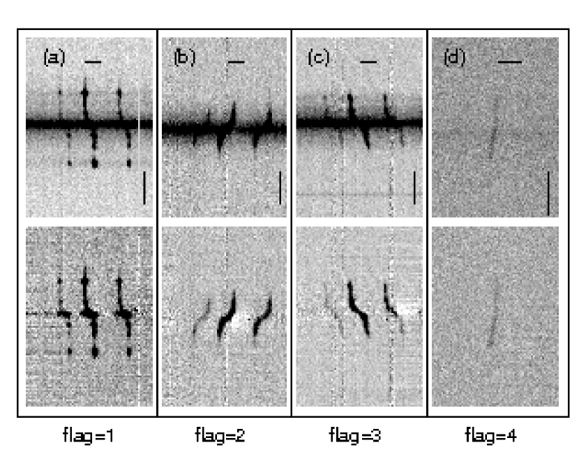
Figure 4: Examples of flat-fielded, wavelength calibrated, and linearized spectra of four galaxies with varying quality flags for their H$\alpha$ rotation curves. Column (a) shows a flag-1 spectrum, with data on the flat portion of the rotation curve. Column (b) shows a flag-2 spectrum, with data extending just past the turn-over radius. Column (c) shows a flag-3 spectrum, with a rising rotation curve at the last detectable data point. Column (d) shows a flag-4 spectrum, with insufficient H$\alpha$ for a useful rotation curve. The horizontal bars indicate 10 Å and the vertical bars indicate 20 arc-seconds. Lower panels show the spectra after continuum subtraction. The central “curve” is the H$\alpha$ emission line used for the rotation curve measurement; (a)-(c) also show the [NII] emission lines.

Accurate measurements of velocity centroids at each spatial position along the slit require accurate removal of the galaxy continuum. A noise image was made that included the galaxy continuum to accurately account for the Poisson noise due to continuum plus H$\alpha$ photons. The galaxy continuum was removed by averaging $\sim$10Å of data on each side of the emission lines, and subtracting this from the area containing the H$\alpha$ emission. Telluric emission lines were subtracted from the data by averaging rows in the spatial direction, where there was no galaxy data, and subtracting that from the area of the CCD containing the galaxy data. Tests using the wavelengths of telluric lines tabulated by Osterbrock et al. (1996) show that the dispersion axis was aligned to be perpendicular to the columns of the CCD to an accuracy of 0.1 Å. Four flat-fielded, wavelength calibrated, and linearized spectra are shown in Figure 4, illustrating varying levels of H$\alpha$ detectability and spatial extent.

Figure 5 compares the rotation curves for the galaxy SDSS J024459.89+010318.5, observed at both Calar Alto and MDM. The overall shapes of the rotation curves are similar, with slightly lower velocities in the MDM data. The two arc-tangent function fits (see §4.1 below) are similar. The arc-tangent fit velocities at 18.4^′′ along the arc-tangent functions, the radius containing 80% of the $i$-band flux (see §4.2), differ by 4.7 $\,{\rm km}\,{\rm s}^{-1}$, about 1.3$\sigma$ (MDM$=186.0\pm 3.3\,\,{\rm km}\,{\rm s}^{-1}$, Calar Alto$=190.7\pm 3.5\,\,{\rm km}\,{\rm s}^{-1}$). The other two galaxies with MDM and Calar Alto spectra show even better agreement in measured rotation speeds than the example shown in Figure 5. We used the Calar Alto rotation curve for this galaxy, because the systematically lower MDM rotation curve suggests a modest slit mis-alignment. Regardless of these small differences there is still overall good agreement between the Calar Alto and MDM data.

4 Measuring Rotation Velocities and Inclination-Corrected Luminosities

4.1 Rotation curve fitting

The procedure to extract rotation curves from the spectra is similar to that used by C97. The 2-D spectra for a galaxy are extracted into 1-D linear spectra, with each 1-D linear spectrum along the spatial direction of the slit being 1 pixel wide ($0.41^{\prime\prime}$ for MDM and $0.55^{\prime\prime}$ for Calar Alto). To avoid assuming an implicit shape of the emission lines, we measure the intensity weighted velocity centroid of the H$\alpha$ line in each 1-D spectrum. The uncertainty in the H$\alpha$ centroid is measured using the signal-to-noise ratio (SNR) at each pixel with H$\alpha$ flux. The H$\alpha$ line centroid has typical uncertainties of $2-12$ $\,{\rm km}\,{\rm s}^{-1}$, depending on the total SNR of the emission line.

Following C97, we fit the observed data points with an arc-tangent function, which has a minimal number of free parameters while adequately describing most galaxy rotation curves over the range probed by H$\alpha$ observations. Specifically, we fit the parameters $V_{0}$, $r_{0}$, $r_{t}$, and $V_{\rm circ}$ of the relation

$$V(r_{i})=V_{0}+\frac{2}{\pi}V_{\rm circ}\mbox{ }{\rm arctan}\left(\frac{r_{i}-r_{0}}{r_{t}}\right)$$ (1)

by minimizing $\chi^{2}$=$\sum_{i}$ $[$ $V(r_{i})$-$V_{\rm obs}(r_{i})$ $]^{2}$/$\sigma_{i}^{2}$, where $V_{0}$ is the systemic velocity, $r_{0}$ is the spatial center of the spectrum, $r_{t}$ is a turn-over radius where the rotation curve goes from steadily rising to flat, $V_{\rm circ}$ is the asymptotic circular velocity, $V_{\rm obs}(r_{i})$ is the intensity weighted velocity centroid at pixel $r_{i}$, and $\sigma_{i}$ is its uncertainty. Note that we do not force $r_{0}$ to correspond to the photometric center of the galaxy. We use a Levenberg-Marquardt minimization routine (Press et. al., 1992), with initial guesses made by eye, to obtain the best-fit parameters and an error covariance matrix. Since galaxy disks have non-circular motions at the $10-20$ $\,{\rm km}\,{\rm s}^{-1}$ level and we do not want the fit dominated by the high SNR data points at the inner parts of the rotation curve, we add 10$\,{\rm km}\,{\rm s}^{-1}$ in quadrature to all the velocity centroid uncertainties. Changing 10$\,{\rm km}\,{\rm s}^{-1}$ to 20 $\,{\rm km}\,{\rm s}^{-1}$ makes a negligible difference in the best-fitting parameters. Changing 10$\,{\rm km}\,{\rm s}^{-1}$ to 0$\,{\rm km}\,{\rm s}^{-1}$ makes little difference in most but not all cases. The typical $\chi^{2}$/d.o.f. is $0.1-1.0$ when 10$\,{\rm km}\,{\rm s}^{-1}$ is added to the centroid uncertainty and $1-2$ without this addition.

Rotation curves are assigned flags indicating how well the data sample the flat part of the rotation curve. Flag-1 indicates that there are data along the flat part of the rotation curve. Flag-2 indicates that there are data at the turn-over radius, but not beyond. Flag-3 indicates that an arc-tangent function adequately describes the data but the rotation curve is still rising at the last measured data points. We assign flag-4 to all galaxies with rotation curves either cannot be fit by an arc-tangent function, or have no detectable H$\alpha$. Although the flags are assigned by eye, the flag correlates well with the difference between the fit parameter $V_{\rm circ}$ and the velocity ($V_{\rm end}$) at the last measured point of the rotation curve. Out of 234 galaxies, there are 64 flag-4, 50 flag-3, 57 flag-2, and 63 flag-1 rotation curves.

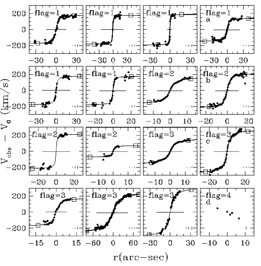
Figure 6: Rotation curves of 16 sample galaxies. The data quality flag is marked in each panel, and the four galaxies shown in Figure 4 appear in the right hand column. Vertical line segments in each panel show the 10th-percentile, median, and 90th-percentile values of the 1$\sigma$ error bars on the observed velocity centroids. Solid curves show the best-fit arc-tangent functions. Open squares mark the fitted velocity at the radius enclosing 80% of the $i$-band flux, which is our standard measure of the galaxy rotation speed. Horizontal bars extend from $-2.2R_{d}$ to $+2.2R_{d}$, where $R_{d}$ is the disk exponential scale length of the $i$-band GALFIT model.

Figure 6 shows rotation curves and best-fit arc-tangent functions for 16 galaxies with flags 1 through 4; the four galaxies whose 2-D spectra appear in Figure 4 are shown in the right-hand column. Vertical line segments in each panel show the 10th-percentile, median, and 90th-percentile values of the 1$\sigma$ error bars on the observed velocity centroids; typical values are 4.5 $\,{\rm km}\,{\rm s}^{-1}$, 5.6 $\,{\rm km}\,{\rm s}^{-1}$, and 11.0 $\,{\rm km}\,{\rm s}^{-1}$. The arc-tangent curves provide good descriptions of the overall shape of the rotation curve in all cases, but some rotation curves show “bumps and wiggles” associated with non-circular motions. As discussed below, our primary measure of galaxy rotation speed is the value $V_{\rm 80}$ of the arc-tangent fit at the radius containing 80% of the $i$-band flux. This point is marked by an open square in each panel. The horizontal lines have a full width of twice 2.2$R_{d}$, where $R_{d}$ is the disk exponential scale length (see §4.3).

4.2 Rotation Speed Definitions

For TF purposes, we want to characterize the fitted rotation curve by a single rotation velocity. While the asymptotic circular speed $V_{\rm circ}$ seems the obvious quantity to use when the rotation curve is fully constrained, the fitted value can vastly overestimate the true rotation speed when the observed data points do not reach the flat portion of the rotation curve. The velocity $V_{\rm end}$ evaluated from the arc-tangent function at the location of the last data point always provides a well constrained rotation speed, with no extrapolation of the model fit, and it maximizes use of the data on each individual galaxy rotation curve. However, $V_{\rm end}$ is difficult to model theoretically, because the spatial extent of the H$\alpha$ data varies from galaxy to galaxy. A common choice for optical rotation curves is the rotation speed $V_{2.2}$ at 2.2 disk scale lengths, where the rotation curve of a self-gravitating exponential disk would peak. We used this measure in our earlier paper for the disk-dominated subset of the galaxy sample (P05). However, for galaxies with significant bulges, the value of $R_{d}$ is sensitive to the degeneracies of bulge-disk decomposition, so we do not want to adopt $V_{2.2}$ as our primary velocity measure for the full sample.

After considering a variety of options, we chose to evaluate the arc-tangent function at a radius ($R_{80}$) containing 80% of the $i$-band flux. This velocity measure, which we refer to as $V_{\rm 80}$, allows a relatively straightforward comparison to galaxy formation theories. For a pure exponential disk, $R_{80}$ is 3.03$R_{d}$, but $R_{80}/R_{d}$ is smaller for galaxies with significant bulges. The empirical logic of choosing $R_{80}$ is evident from Figure 6: most of our rotation curves extend close to or beyond $R_{80}$, so substantial extrapolation of the rotation curve is rarely required, and it is far enough out to be close to $V_{\rm circ}$ in most cases.

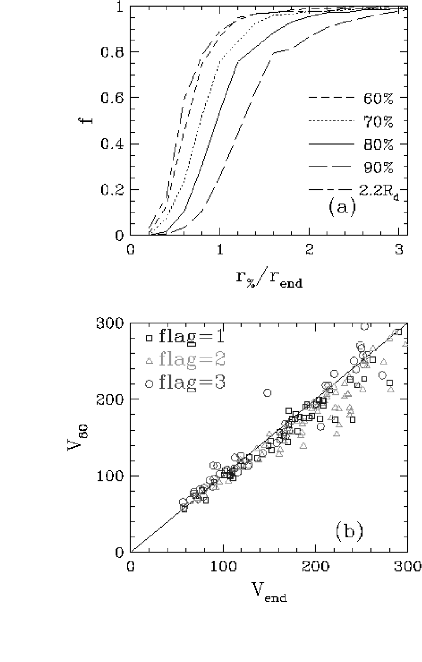
Figure 7: (Top) Cumulative distributions of the radii that contain 60%, 70%, 80%, and 90% of the $i$-band flux divided by the radius of the last H$\alpha$ data point. The distribution for 2.2$R_{d}$ is also shown. (Bottom) Comparison of our standard velocity measure $V_{\rm 80}$, the value of the arc-tangent function evaluated at the radius containing 80% of the $i$-band flux, to $V_{\rm end}$, the velocity evaluated at the radius of the last H$\alpha$ data point.

Figure 7a makes this point quantitatively, showing the cumulative distribution of 2.2$R_{d}$ and the radii containing 60%, 70%, 80%, and 90% of the $i$-band flux divided by the radius $R_{\rm end}$ of the outermost H$\alpha$ data point. Half of the galaxies have data extending beyond $R_{80}$. The radii 2.2$R_{d}$, $R_{60}$, and $R_{70}$ would under-utilize the data for a large fraction of the sample and be further from $V_{\rm circ}$, while evaluating the velocity at $R_{90}$ would require extrapolation in most cases. Figure 7b shows a generally good correlation between $V_{\rm 80}$ and $V_{\rm end}$, with a handful of flag-3 galaxies having $V_{\rm 80}$ significantly greater than $V_{\rm end}$, and some flag-1,2 galaxies with extended rotation curves having $V_{\rm end}$ $>$ $V_{\rm 80}$. Our choice of $V_{\rm 80}$ as a rotation speed definition is very similar to that of Persic, Salucci, & Stel (1996) and Catinella, Giovanelli, & Haynes (2006), who evaluate the rotation curve at the radius containing 83% of total flux (see Catinella, Haynes, & Giovanelli (2005) for further discussion). In Appendix A, we present TF fits for the alternative velocity definitions $V_{2.2}$ and $V_{\rm end}$.

4.3 Bulge-Disk Decomposition

Bulge and disk parameters of our target galaxies are needed for three reasons: to correct the measured velocities ($V_{\rm 80}$) for disk inclination, to correct absolute magnitudes for internal extinction by dust in the disk, and to obtain structural quantities that can be tested for correlations with TF residuals. The DR2 isophotal axis ratio may be affected by the presence of a bulge and spiral arms. Therefore, refitting the disk, separate from the bulge, provides more accurate disk axis ratios for the inclination correction of the velocities and the internal disk extinction correction. The bulge-disk decomposition also allows measurements of the disk size and surface brightness, which are possible third parameters in the TF relation.

We fit a Sersić profile (Sersić, 1968) to the bulge and an exponential profile to the disk, using the two-dimensional profile fitting program GALFIT (Peng et al., 2002). We run GALFIT on the $g$, $r$, and $i$-band images of our galaxies, holding the disk profile fixed as an exponential disk and leaving the bulge Sersić index $n$ as a free parameter. The Sersić index describes the central concentration of the light profile, with $n$=1 for an exponential disk and $n$=4 for a DeVaucouleurs profile. We run GALFIT setting the initial bulge Sersić concentration equal to $n$=2 and visually inspect the results. The $\chi^{2}$ is sensitive to small-scale asymmetries and variations in the galaxy profile that are not two-dimensionally symmetric (i.e. HII regions, spiral arms, and bars), so visual inspection of the fit results is required to ensure that GALFIT does not drift to a local $\chi^{2}$ minimum in an un-realistic location of parameter space. Masking out strongly asymmetric features and re-running GALFIT resolves these problems when they arise.

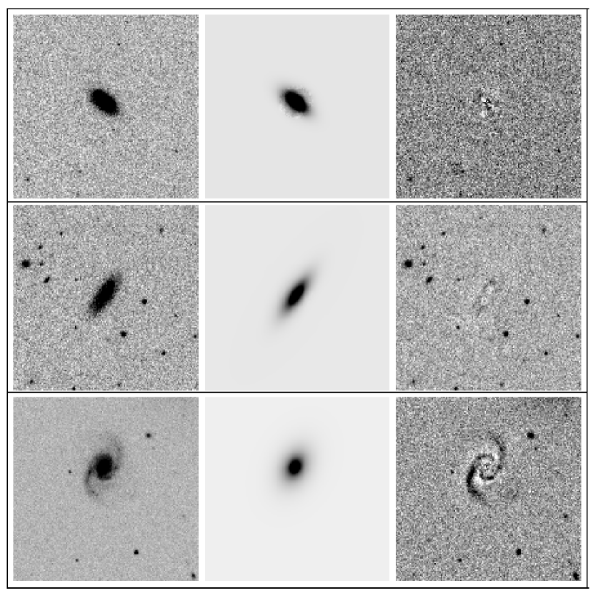
Figure 8: Two-dimensional bulge-disk decomposition of the $i$-band images of J235656.66-005912.3, J094949.62+010533.2, J135946.01+010432.8 (top to bottom). From left to right the panels are the data, the GALFIT model, and the residual image given by subtracting the GALFIT model from the data.

Figure 8 shows examples of 2-D symmetrical Sersić profile fits to our flag-1,2,3 galaxies. The top and middle rows show typical results for galaxies that do not have prominent spiral arms. The bottom panel shows a result for a galaxy that has prominent spiral arms. Since our galaxies are selected to be inclined, we rarely find prominent bars in the images.

Figure 9 shows 1-D profiles along the major axis of the data, model, and residual images for galaxies shown in Figure 8. From Figure 9 we can conclude that our best-fit models accurately describe the galaxy surface brightness profiles down to $\sim$25 mag/arcsec² or fainter, except for small scale variations. The bulge-to-disk flux ratio, disk axis ratio, and disk position angle are generally robust outcomes of the fitting procedure, converging quickly with little sensitivity to the initial parameter choice. The bulge radius, Sersić index, and position angle are subject to more uncertainty, in part because the bulge component is often similar in size to the seeing FWHM. Figure 10 shows that approximately 20% of our galaxies with usable rotation curves have significant bulges, where early-type galaxies have concentrations around 2.6. Figure 10 also shows that galaxies with lower concentrations tend to have higher disk-to-total flux fractions. A visual inspection of the flag-1,2,3,4 galaxies confirms this trend, where the flag-3,4 galaxies tend to have early morphological types. The flag-1 galaxies are predominantly Sb and Sc Hubble types, whereas the flag-4 galaxies are predominantly Sa with a few Sc galaxies. The flag-2,3 galaxies are mixed between Sa, Sb, and Sc types.

4.4 Internal Extinction Corrections

Dust in galaxy disks absorbs a larger fraction of the disk light in edge-on directions. Therefore, it is standard practice to apply internal extinction corrections to luminosities used for the TF relation. We follow this practice here and use the Tully et al. (1998) formulation adapted to our bands. We apply internal extinction corrections to the disk, while assuming that the bulge has no correction to the face-on value because it has little dust. Tully et al. (1998) provide prescriptions for the internal extinction corrections in the Johnson $B$ (438 nm), $R$ (641nm), $I$ (798 nm), and $K^{\prime}$ filters as a function of the galaxy inclination and the absolute magnitude in that band. We convert the SDSS $g$ (469 nm), $r$ (617nm), $i$ (748nm), and $z$-band (893 nm) absolute magnitudes to Johnson magnitudes using the conversions in Table 7 of Smith et al. (2002), then linearly interpolate the Tully et al. (1998) corrections back from the Johnson central wavelengths to the SDSS central wavelengths as listed above. This internal extinction correction is then applied to the disk $g$, $r$, $i$, and $z$-band disk fluxes, which are then added to the un-corrected bulge fluxes.

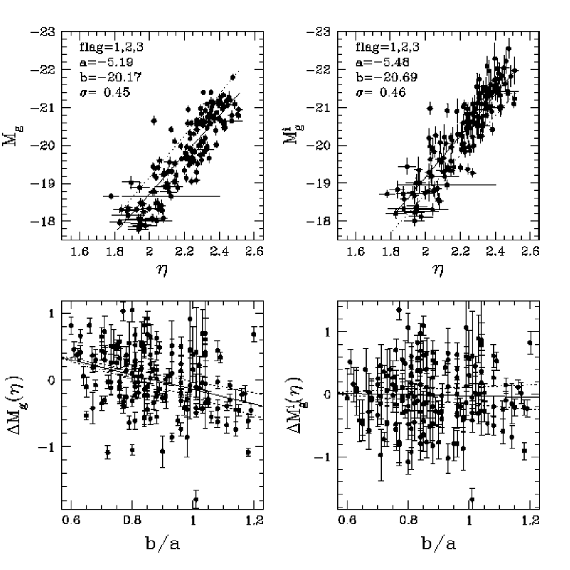
Figure 12: Effect of the internal extinction correction on the $g$-band TF relation. Upper panels show the data (points) and best-fit TF relations (solid lines) without (left) and with (right) internal extinction corrections. The dotted line shows the fit from the other panel. Lower panels plot TF residual against $i$-band axis ratio, with solid lines showing the best-fit trend and dotted lines the bootstrap-estimated uncertainty. We define $\eta\equiv\log V_{\rm 80}/(\,{\rm km}\,{\rm s}^{-1})$, where $V_{\rm 80}$ is the inclination corrected circular velocity at the radius containing 80% of the $i$-band flux.

Figure 11 shows histograms of the total internal extinction correction in each band. Typical values of the $g$-band internal extinction range from 0.2 to 0.8 magnitudes. The median internal extinction correction decreases from 0.6 in the $g$-band to 0.2 in the $z$-band. Figure 12 shows the $g$-band TF relation with and without the internal extinction correction. Solid lines show fits using the maximum likelihood procedure discussed in §5 below. The slope of the extinction-corrected TF relation is similar to the uncorrected slope ($-5.5\pm 0.2$ versus $-5.2\pm 0.2$), though of course the extinction correction increases the zero point by the average value of the extinction. The lower panels of Figure 12 show that the internal extinction correction successfully removes a weak trend of TF residual with axis ratio, so it appears to be a valid and useful correction on average, even if it is uncertain on a galaxy by galaxy basis. We assume, somewhat arbitrarily, that the inclination correction uncertainty is 1/3 of the correction itself. Results in Appendix A show that, with this assumed observational uncertainty, the internal extinction corrections do not change the inferred intrinsic scatter $\sigma$. All magnitudes discussed in the remainder of the paper have this correction applied.

4.5 Error Budget

We are ultimately interested in the slope, intercept, and intrinsic scatter of the TF relation. To estimate these, we need an accurate characterization of the observational errors of our data. This is especially important for estimating intrinsic scatter, since the total scatter about the fitted relation is, roughly speaking, the quadrature sum of the intrinsic scatter and the observational errors.

The TF relation is the correlation of the logarithm of the rotation velocity with the absolute magnitude. We define the logarithm of the rotation velocity to be

$$\eta\equiv\log\left(\frac{V_{\rm 80}}{\sin i(1+z)}\right),$$ (2)

where $i$ is the disk inclination angle inferred from the bulge-disk decomposition procedure described in §4.3, and the $(1+z)$ term accounts for cosmological broadening. We relate the inclination to the observed axis ratio using the equation

$$\sin i=\sqrt{\frac{1-(b/a)^{2}}{1-0.19^{2}}},$$ (3)

where $b/a$ is the $i$-band disk axis ratio determined using GALFIT, and $0.19$ takes into account the finite thickness of the disk (see the discussion in Haynes & Giovanelli (1984)); varying $0.19$ over the range 0.10$-$0.25 causes the inclination correction to vary by $<$ 1.5%. We define the absolute magnitude to be

$$M_{\lambda}\equiv m_{{\rm Petro},\lambda}-5\log_{10}(d_{\rm lg}/(1+z))+5-A_{\lambda}^{i}-A_{\lambda}^{\rm MW}+K_{\rm corr,\lambda},$$ (4)

where $\lambda$ denotes the band ($g$, $r$, $i$, or $z$), $m_{{\rm Petro},\lambda}$ is the SDSS Petrosian magnitude in the $\lambda$-band, $A_{\lambda}^{i}$ is the internal extinction correction described in §4.4, $A_{\lambda}^{\rm MW}$ is the correction for Milky Way extinction taken from the SDSS database (based on Schlegel, Finkbeiner, & Davis 1998), $K_{\rm corr,\lambda}$ is the K-correction from Blanton et al. (2003b), and $d_{\rm lg}$ is the luminosity distance to the galaxy from the Local Group. As noted earlier, we compute distances using the SDSS heliocentric redshifts corrected to the rest frame of the Local Group barycenter (Yahil, Tammann, Sandage 1977), assuming a cosmological model with $\Omega_{m}=0.3$, $\Omega_{\lambda}=0.7$, and $h=0.7$. There are six galaxies (J233152.99-004934.4, J144418.37+000238.5, J095555.07-001125.0, J112346.06-010559.4, J203523.80-061437.9, J001006.62-002609.6) that have poorly estimated Petrosian magnitudes in the DR2 photometric pipeline. For these galaxies, we use the total Sersić magnitude measured using GALFIT.

The uncertainty in the absolute magnitude is calculated using standard propagation of errors,

$$(\delta M_{\lambda})^{2}=(\delta m_{\rm petro,\lambda})^{2}+\left(5\times 0.434\frac{\delta z}{z}\right)^{2}+\left(5\times 0.434\frac{\delta V_{\rm pec}}{cz}\right)^{2}+(\delta A_{\lambda}^{i})^{2},$$ (5)

where 0.434 converts from natural to base-10 logarithms. Uncertainties in apparent magnitude $\delta m_{\rm petro,\lambda}$ and redshift $\delta z$ are taken from the DR2 database, though we impose a minimum redshift error of $c\delta z$ $=$ 30 $\,{\rm km}\,{\rm s}^{-1}$. The uncertainty in the Milky Way foreground extinction, $A_{\lambda}^{MW}$, is assumed to be negligible. We incorporate a distance uncertainty corresponding to $\delta V_{\rm pec}$ = $300$ $\,{\rm km}\,{\rm s}^{-1}$ when calculating disk scale length and luminosity uncertainties, to account for the typical amplitude of small scale peculiar velocities (Strauss & Willick 1995). We assume the uncertainty due to the internal extinction correction is one third of the calculated value, $\delta A_{\lambda}^{i}$ = $A_{\lambda}^{i}$/3, and we ignore any (much smaller) uncertainty due to the uncertainty in the GALFIT determined $i$-band axis ratio. In practice, peculiar velocity and internal extinction uncertainties completely dominate the uncertainty in $M_{\lambda}$. The 10-th, median, and 90-th percentile values of the peculiar velocity uncertainty, $5\times 0.434\frac{\delta V_{\rm pec}}{cz}$, are 0.049, 0.080, and 0.118, respectively. The 10-th, median, and 90-th percentile total $i$-band internal extinction correction uncertainties are 0.041 mag, 0.088 mag, and 0.16 mag, respectively.

The velocity width has uncertainties due to the inclination correction, measurement of $V_{\rm 80}$ from the rotation curve, and possible systematic uncertainties due to slit misalignment. As described in §2, we removed six galaxies from our sample for which misalignment could cause a $>$10% change in the circular velocity; we do not correct six other galaxies with slight slit misalignments for which the correction is $<$10%. The uncertainty in the inclination corrected velocity width ($V_{80,i}$) due to the inclination uncertainty and uncertainties in the measurement of $V_{\rm 80}$ is

$$\left(\frac{\delta V_{80,i}}{V_{80,i}}\right)^{2}=\left(\frac{\delta V_{\rm 80}}{V_{\rm 80}}\right)^{2}+\left(\frac{\delta(b/a)(b/a)}{1-(b/a)^{2}}\right)^{2}~{}.$$ (6)

The first term dominates for essentially all of the galaxies. Using the covariance matrix returned by the Levenberg-Marquardt method, the uncertainty of the arc-tangent function measured at $R_{80}$ is related to the uncertainty in the arc-tangent function parameters via the equation

$$\delta V_{\rm 80}^{2}=\left(\sum_{ij}C_{ij}\frac{\partial^{2}V_{\rm arctan}(R_{80}|a_{i},a_{j})}{\partial a_{i}\partial a_{j}}\right)^{2}.$$ (7)

The indices run from 1 to 4 for the four arc-tangent function parameters $a_{i}$ and $a_{j}$. The axis ratio is determined from the disk component after running GALFIT on the $i$-band corrected frames, with the uncertainty reported by GALFIT. The 10th-percentile, median, and 90th-percentile 1$\sigma$ uncertainties in log $V_{80,i}$ are 0.006, 0.011, and 0.044 ${\rm log_{10}}$(km/sec) respectively. For a TF slope of $-6.0$ mag / ${\rm log_{10}}$ (km/sec), these uncertainties correspond to 0.034, 0.063, and 0.264 mag respectively. A typical uncertainty for our program galaxies is thus $\sim$ 0.063 mag from the $V_{80,i}$ uncertainty, $\sim$ 0.088 mag from the internal extinction correction uncertainty, and $\sim$ 0.080 mag from the peculiar velocity, summing in quadrature to 0.13 mag. This is much smaller than the intrinsic scatter measured in §5.2. However, the variation from galaxy to galaxy is large. For the rest of the paper we will use inclination corrected velocities and drop the subscript $i$ from $V_{80,i}$. Table 2 summarizes the photometric parameters and their errors, and Table 3 summarizes the velocity-width measurements and their errors.

5 The Tully-Fisher Relation

5.1 Modeling the TF Relation

We use a maximum likelihood method to estimate the slope $a$, intercept $b$, and intrinsic scatter $\sigma$ of the TF relation. For the “forward” relation, the independent and dependent variables are $x$ = $\eta$ $\equiv$ ${\rm log}(\frac{V_{\rm 80}}{{\rm sin{\it i}(1+z)}})$ and $y$ = $M_{\lambda}$, respectively. We assume that the intrinsic scatter is Gaussian in form, so that the probability that galaxy $i$ has a true absolute magnitude $y_{i}$ given a true velocity width $x_{i}$ is

$$p(y_{i}|x_{i})=(2\pi\sigma^{2})^{-1/2}{\rm exp}\left[\frac{-(y_{i}-\overline{y_{i}})^{2}}{2\sigma^{2}}\right],$$ (8)

where

$$\overline{y_{i}}=a(x_{i}-x_{0})+b$$ (9)

is the mean value expected for a linear TF relation with parameters $a$ and $b$. The value of $x_{0}$ is chosen so that there is no correlation (or very little correlation) between the statistical errors in $a$ and $b$. For the “inverse” TF relation, we adopt the same model but with $x$ = $M_{\lambda}$ and $y$ = $\eta$. The forward and inverse relations correspond to different assumptions about which physical parameter is “primary”: in the forward relation, the absolute magnitude has Gaussian scatter about a mean value determined by the linewidth, and the reverse holds for the inverse relation.

We assume that the observational estimates of $\hat{x_{i}}$ and $\hat{y_{i}}$ are Gaussian distributed about the true values of $x_{i}$, $y_{i}$, i.e.,

$$p(\hat{y_{i}}|y_{i})=(2\pi\sigma_{y,i}^{2})^{-1/2}{\rm exp}\left[\frac{-(\hat{y_{i}}-y_{i})^{2}}{2\sigma_{y,i}^{2}}\right]$$ (10)

and

$$p(\hat{x_{i}}|x_{i})=(2\pi\sigma_{x,i}^{2})^{-1/2}{\rm exp}\left[\frac{-(\hat{x_{i}}-x_{i})^{2}}{2\sigma_{x,i}^{2}}\right],$$ (11)

where $\sigma_{x,i}$, and $\sigma_{y,i}$ are the measurement uncertainties determined as described in §4.5. The values of $a$, $b$, and $\sigma$ can then be estimated by maximizing the log-likelihood

$${\rm ln}\,L=\sum_{i}{\rm ln}\,p(\hat{y_{i}}|\hat{x_{i}},\sigma_{x,i},\sigma_{y,i}).$$ (12)

The likelihood for an individual data point can be written

$$p(\hat{y_{i}}|\hat{x_{i}}) = \int_{-\infty}^{\infty}dy_{i}\,p(\hat{y_{i}}|y_{i})p(y_{i}|\hat{x_{i}}),$$ (13)

$$= \int_{-\infty}^{\infty}dy_{i}\,p(\hat{y_{i}}|y_{i})\int_{-\infty}^{\infty}dx_{i}\,p(y_{i}|x_{i})p(x_{i}|\hat{x_{i}}).$$

We set $p(x_{i}|\hat{x_{i}})$ $=$ $p(\hat{x_{i}}|x_{i})$, implicitly assuming a flat prior for $p(x_{i})$ over the (typically narrow) range of values allowed by the uncertainty in $\hat{x_{i}}$. Substituting equations (8)-(11) and (13) into (12) and simplifying yields the expression

$${\rm ln}\,L=-\frac{1}{2}\sum_{i}{\rm ln}\,(\sigma^{2}+\sigma_{y,i}^{2}+a^{2}\sigma_{x,i}^{2})-\sum_{i}\frac{[\hat{y_{i}}-(a\hat{x_{i}}+b)]^{2}}{2(\sigma^{2}+\sigma_{y,i}^{2}+a^{2}\sigma_{x,i}^{2})}+\,{\rm constant}.$$ (14)

Most previous TF studies have implicitly set $\sigma$ to zero when finding the best-fit values of $a$ and $b$, then estimated $\sigma$ after the fact from the difference between the observed scatter and the estimated contribution of observational errors. In the presence of non-zero intrinsic scatter, this method assigns too much weight to the data points with the smallest observational errors, yielding statically non-optimal estimates of $a$ and $b$ and underestimates of their uncertainties. For example, two data points with near-zero errors would completely dominate the fit, while in fact they should be weighted by 1/$\sigma^{2}$. Further discussion of these issues can be found in D’Agostini (2005).

The equation $\delta{\rm ln}L/\delta{\rm ln}b$ $=$ 0 (see eq. 14) can be solved analytically given values of $a$, $\sigma$, and the input data ($\hat{x_{i}},\hat{y_{i}},\sigma_{x,i},\sigma_{y,i}$). We determine the maximum likelihood parameters by performing a grid search in $a$ and $\sigma$, finding the best-fit value of $b$ (analytically) for each ($a$, $\sigma$) combination, then choosing the ($a$, $b$, $\sigma$) combination that maximizes ln$L$. We determine the 1$\sigma$ errors on $a$, $b$, and $\sigma$ by repeating this procedure for 100 bootstrap subsamples of the full data set, taking the dispersion among the bootstrap estimates as the uncertainty in the parameter. We choose the values of $x_{0}$ in equation (9) so that there is essentially no covariance between the error in $a$ and the error in $b$; specifically we choose the value of $x_{0}$ so that fixing $a$ to a value of $\pm$1$\sigma$ from its best-fit value does not change the best-fit value of $b$. The resulting zero-points in the $g$, $r$, $i$, and $z$ TF fits are, respectively, $\eta_{0}$ = 2.22, 2.22, 2.22, 2.23 for the forward fit and $M_{\lambda_{0}}$ = $-20.607$, $-21.107$, $-21.327$, and $-21.400$ for the inverse fit.

5.2 The TF Relation in the SDSS Bands

Figure 13a shows the $i$-band TF relation with 162 flag-1,2,3 data points. The data show a clear linear trend of $M_{i}$ with $\eta$ and an intrinsic scatter larger than the error bars. The best-fit parameters for the forward relation are $a=-6.32\pm 0.22$, $b=-21.390\pm 0.035$ (at $V_{\rm 80}$ = 166.0 $\,{\rm km}\,{\rm s}^{-1}$), and intrinsic scatter $\sigma=0.423\pm 0.035$. Table 4 lists these parameters and the parameters $a_{\rm inv}$, $b_{\rm inv}$, $\sigma_{\rm inv}$ of the inverse fit. When comparing the inverse TF to the forward TF relation in the figures and text, we invert the inverse relation and refer to the slope and scatter by $a^{\prime}$ = $1/a_{\rm inv}$ and $\sigma^{\prime}$ = $\sigma_{\rm inv}$/$a_{\rm inv}$, and quote the intercept $b^{\prime}$ as the value of $M_{\lambda}$ that corresponds to the zero-point $\eta_{0}$ used in the forward fit. The quantities $a^{\prime}$, $b^{\prime}$, $\sigma^{\prime}$ have the same units as $a$, $b$, $\sigma$ and can be directly compared. For the flag-1,2,3 sample, the inverse TF $i$-band relation $a^{\prime}$, $b^{\prime}$, and $\sigma^{\prime}$ are $-7.69\pm 0.29$, $-21.39\pm 0.04$, and $0.47\pm 0.04$. For all bands and samples, the inverse relation has a steeper slope than the forward relation but similar scatter (see discussion in §5.3 below). Throughout the paper we use the terms “steep” and “shallow” in reference to the slope (more negative is steeper) of the forward TF relation ($V_{\rm 80}$ predicting $M_{\lambda}$).

Figure 13b,c shows the $i$-band TF relation when less spatially extended rotation curves (flag-2,3) are removed. As flag-3 and then flag-2 galaxies are removed, the slope becomes slightly shallower, changing from $-6.32\pm 0.22$ to $-6.02\pm 0.32$ to $-5.94\pm 0.44$. The change is at the $\sim$ 1$\sigma$ level, and it is driven largely by the change in the sample luminosity distribution, as there are fewer flag-1,2 galaxies at low luminosity. Similar trends are seen in $g$, $r$, and $z$. The intrinsic scatter declines by a statistically insignificant amount, from 0.42$\pm$0.04 to 0.39$\pm$0.05 from flag-1,2,3 to flag-1 only. The constancy of $\sigma$ implies that our fitting procedure gives a reasonable estimate of the uncertainty in $V_{\rm 80}$ even for rotation curves that are rising at the outermost point. Given the insensitivity of the results to including flag-2,3 galaxies, we will use the full sample henceforth, for improved statistics and greater sample completeness. We list TF parameters for the flag-1,2 sample in Table 6 (see Appendix A).

Figure 14 shows the TF relation for the $g$, $r$, $i$ and $z$-bands, with parameters fit to the data as outlined in §5.1. The forward TF slope increases towards the redder bands, from $-5.48$ to $-6.59$, a change much larger than the statistical slope uncertainties (typically 0.2). This is the expected trend, as fainter galaxies typically have bluer colors. Trends in the intercept are not particularly meaningful, as they depend on the adopted (AB) magnitude system and stellar mass-to-light ratios in different wavebands. The inverse TF slopes are always steeper than the forward slopes, and they show the same trend with wavelength. The intrinsic scatter is slightly larger in the $g$-band, and roughly constant in $r$, $i$, and $z$. This constancy implies that the extinction corrections are not an important source of scatter. It further suggests that the intrinsic scatter is not dominated by variations in stellar populations, a point we will return to in §6 below. Excluding flag-3 and flag-2 galaxies in the $g$, $r$, and $z$-bands shows the same trends seen in Figure 13. TF fits using velocity width definitions $V_{2.2}$ and $V_{\rm end}$ are discussed in Appendix A.

As shown in §2 (cf. Figure 1), the $M_{r}$ distribution of our sample is approximately flat in the range $-18.5>M_{r}>-22$, but not exactly so. In order to provide a well defined target for galaxy formation theories, we have also computed TF parameters after weighting galaxies to obtain the results expected for a truly flat $M_{r}$ distribution. Using the plotted distribution of galaxies in 0.5-magnitude bins, we give each galaxy a weight $w_{i}$ defined as the ratio of the number of galaxies in the most populated bin to the number of galaxies in its bin. These weights are incorporated into the fitting procedure by multiplying each term inside the sums of equation (14) by $w_{i}$, as though we had observed the galaxy $w_{i}$ times ($w_{i}$ goes inside the ln of the first term). The weights vary from 1 to 5, depending on the bin. We do not include the few galaxies with $M_{r}$ $>$ $-18.5$ and $M_{r}$ $<$ $-22$. The results are quoted in Table 6. Overall, the parameters change very little when weighted by our observed $M_{r}$ distribution. We have carried out a similar weighting experiment to examine the effect of exactly reproducing the $g$-$r$ color distribution of the DR4 “control” sample shown by the dotted curve in Figure 3a. The change in the TF parameters (not listed) is much smaller than our statistical errors.

Our sample has absolute magnitude cuts that can create Malmquist-type biases in TF estimates. The explicit absolute magnitude-redshift cuts outlined in §2, and the flag-1,2,3 absolute magnitude distribution seen in Figure 1, may cause a shallowing of a TF slope and reduction of the intrinsic scatter when these cuts are applied to data having non-zero scatter. Random errors in galaxy distances and scatter across selection boundaries, due to peculiar velocities typically of the order 300 $\,{\rm km}\,{\rm s}^{-1}$, can also induce Malmquist-type biases in TF estimates. Appendix B describes a Monte Carlo experiment aimed at testing for such biases inherent in our sample, assuming a power-law TF relation with Gaussian intrinsic scatter. In short, generating a Monte Carlo sample with an input $a$ $=$ -7.35, $b$ $=$ -21.27, and $\sigma$ $=$ 0.58, then applying the selection criteria outlined above, yields a best-fit forward relation of $a$ $=$ -6.32, $b$ $=$ -21.39, and $\sigma$ $=$ 0.42 which is close to the observed $i$-band TF relation (Table 4). The difference between the input and best-fit forward relations is several times our statistical uncertainties. The difference between the inverse relations is small. In this paper we present a TF relation for a sample of galaxies with well defined selection criteria, enabling a theory to reproduce our sample, using our selection criteria, in an attempt to model our measured TF relation. Table 4 represents the TF parameters measured with our selection criteria.

5.3 Intrinsic Scatter

One of our principal objectives is a robust estimate of the intrinsic scatter of the TF relation for a broadly selected sample of galaxies. Previous observational studies have shown a very wide range of estimates, with some as low as 0.1 to 0.15 mags (Bernstein et al., 1994). For a large sample of late-type spirals, with similar analysis methods to those used here, C97 reports 0.46 mag of total (intrinsic $+$ observational) $r$-band scatter. K02 calculates and $R$-band intrinsic scatter of 0.4 mag for the broadly selected Nearby Field Galaxy Survey (Jansen & Kannappan, 2001) and Ursa Major samples, after the selection criteria are matched. However, V01 reports a much smaller scatter, 0.15 $-$ 0.18 mag in $R$-band, for galaxies in the Ursa Major cluster, using the flat part of the HI rotation curve as the circular velocity measure (see Table 6 of V01). This estimate arises after subtracting 0.17 mag of scatter attributed to the depth of the cluster, and changes to the sample or velocity width definition can boost the $R$-band scatter in the V01 analysis as high as 0.54 mag. Observational estimates from other studies span the full range of values quoted above (see e.g., the review by Strauss & Willick 1995).

Many papers do not clearly distinguish the intrinsic scatter from the total scatter. In part, the observational errors themselves can be difficult to estimate for nearby samples in which distance errors dominate and are difficult to define precisely. In addition, previous studies have generally not estimated the intrinsic scatter as part of the TF fitting procedure as we have done, but have rather subtracted a “typical” observational error in quadrature from the total scatter.

A crucial feature of our sample is that the typical observational errors are smaller than the intrinsic scatter because we are measuring galaxies with $V$ $>$ $5000$ $\,{\rm km}\,{\rm s}^{-1}$ and have photometry that allows precise estimates of magnitudes and axis ratios. The most debatable elements of our observational error budget (see §4.5) are the $300\,{\rm km}\,{\rm s}^{-1}$ peculiar velocity error and the internal extinction error of $1/3$ the internal extinction correction. These typically contribute 0.080 and 0.088 mag to the absolute magnitude error. If we increase the assumed peculiar velocity uncertainty from 300 to 500 $\,{\rm km}\,{\rm s}^{-1}$, per galaxy, our estimate of the $i$-band intrinsic scatter decreases from 0.42 to 0.40 mag. If we set the assumed internal extinction error to zero, the estimated intrinsic scatter increases from 0.42 to 0.43 mag. Thus, our estimate of $\sigma$ is relatively insensitive to the uncertain elements of our error budget. Even if we take the drastic step of setting all of our observational errors to zero, the best-fit intrinsic scatter only increases to 0.48 mag.

When computing inclination corrected velocities, we take the uncertainty in $\sin i$ from the uncertainty in the axis ratio of the GALFIT bulge-disk decomposition. We thus implicitly assume that the disk is adequately described by a circularly symmetric exponential, and disk ellipticities by definition contribute to the intrinsic rather than the observational scatter. Zaritsky & Rix (1995), from a study of face-on galaxies, estimate typical ellipticities of $\sim$ 0.05 for the gravitational potential in the disk plane, which would cause $\sim$ 0.15 mag of TF scatter from a combination of inclination correction errors and non-circular motions (see also Franx & de Zeeuw 1992; Ryden 2005).

Since we have broader sample selection than most previous studies, it is interesting to ask whether outliers have an important impact on the TF scatter (or other TF parameters). Figure 15a shows the $i$-band TF relation with the seven top contributors to $\chi^{2}$ marked. From largest to smallest $\Delta$$\chi^{2}$ they are J021941.13-001520.4, J235106.25+010324.0, J124428.85-002710.5, J204913.40+001931.0, J005650.61+002047.1, J013142.14-005559.9, and J235607.82+003258.1. None of these galaxies show obvious rotation curve anomalies, but some are morphologically unusual. J021941.13-001520.4 has extended and asymmetrical spiral arms, and its GALFIT axis ratio is 0.51, giving it a substantial inclination correction. It is therefore possible that the low rotation speed of this galaxy arises from an inaccurate inclination correction. The second galaxy, J235106.25+010324.0, has normal morphology, as does the fifth galaxy J005650.61+002047.1. The third galaxy, J124428.85-002710.5, has a prominent central point source that produces a persistent residual in the bulge-disk decomposition. However, it is under-luminous relative to the mean TF relation, so an AGN contribution cannot explain the anomaly. The fourth galaxy, J204913.40+001931.0, has a prominent dust lane, as does the sixth, J013142.14-005559.9. Finally J235607.82+003258.1 has a large ring $\sim$ 28 kpc in size centered on the galaxy. However, there are other galaxies with dust lanes or morphological asymmetries that are not TF outliers, so we do not think that the intrinsic scatter of the sample is simply driven by rare “oddballs”.

Figure 15b shows the impact of removing, in succession, the data points with the lowest likelihood (beginning with the seven shown in Figure 15a), then refitting the TF relation. Filled circles show the estimated forward scatter as data points are removed, while open circles show the corresponding quantity $\sigma^{\prime}$ $=$ $\sigma_{\rm inv}$/$a_{\rm inv}$ of the inverse relation. The inset panel shows the best-fit slopes $a$ and $a^{\prime}$ $=$ 1/$a_{\rm inv}$. Removing the first data point, J021941.13-001520.4, produces a noticeable drop in $\sigma$, from 0.42 to 0.40 mag. Since our estimated inclination for this galaxy could be inaccurate for the reasons mentioned above, we think there is a reasonable case for lowering our estimated values of the intrinsic TF scatter by $\sim$ 0.02 mag (less than our statistical uncertainty of $\sim$ 0.035 mag). However, removing subsequent data points produces only a steady, approximately linear decrease of the estimated intrinsic scatter. If the TF residuals were drawn from a Gaussian of width 0.4 mag, then the estimated scatter should show an approximately linear decrease to zero at N_removed $=$ 160 (a claim we have tested with Monte Carlo experiments). The fact that our estimated scatter goes to zero at N_removed $\approx$ 90 suggests that we may have overestimated the observational errors. If we set the internal extinction correction and peculiar velocity uncertainties to zero and repeat the above procedure, the estimated scatter of the forward TF relation approaches zero at N_removed $\sim$ 130.

Closely related to the role of outliers is the question of the residual distribution. Figure 16 plots the histograms of $\Delta$$y$/$\sigma_{T}$, where $\Delta$$y$ is the deviation of each galaxy from the mean forward (solid) or inverse (dotted) relation and $\sigma_{T}$= $[\sigma^{2}+\sigma_{y}+a^{2}\sigma_{x}^{2}]^{1/2}$ is the quadrature sum of the intrinsic scatter and the galaxy’s observational error. With the exception of the one largest outlier in the forward and inverse relations, both histograms are approximately Gaussian in form. (The largest outlier galaxy has $\Delta$$y$/$\sigma_{T}$ $=$ $-4.2$.) This is further evidence that the intrinsic scatter of our sample is not driven by rare outliers.

Although the differing slopes of the forward and inverse relation (specifically, the fact that $a$ $\neq$ 1/$a_{\rm inv}$) makes them appear superficially different, Figure 16 shows that they both lead to nearly Gaussian residual distributions. The forward and inverse relations with Gaussian intrinsic scatter are equally good, and essentially equivalent, descriptions of the two-dimensional distribution of galaxies in the ($M_{\lambda}$,$\eta$) plane, over the range covered by our sample. Theoretical models of the galaxy population should explain this full distribution, not just a slope and intercept whose values necessarily depend on the fitting procedure. Similarly, there is no particular virtue to “orthogonal” fitting procedures that treat the two observables symmetrically – they would have intermediate slopes, but they would presumably lead to a similar two-dimensional distribution once the scatter was properly accounted for.

Our estimate of $\sigma=0.42$ mag (for the flag-1,2,3 $i$-band forward relation) is larger than at least some previous estimates of the TF intrinsic scatter. It is interesting to explore whether this is a consequence of our broader morphological selection. Figure 17 compares the $i$-band TF relation of our full sample to a disk-dominated subset that have, according to the GALFIT bulge-disk decomposition, $i$-band disk-to-total flux fractions $D/T$ $\geq$ 0.9 (see P05 for an extensive discussion of this subset). The intrinsic scatter drops to $\sigma$ $=$ 0.36 mag, a statistically significant but modest decrease. Selecting disk-dominated systems does not yield the small values of the intrinsic scatter found in some previous studies. We do not see any clear evidence for a luminosity dependence of the intrinsic scatter (Giovanelli et al., 1997), but our sample is relatively small for detecting such an effect.

Figure 17b shows the $g$-band TF relation of the full sample, with barred, asymmetric, and “interacting” galaxies marked separately. Barred galaxies are identified by visual inspection of the $i$-band images, since bars are usually red. We find 17 galaxies with discernible bars, but this is an under-estimate of the true barred fraction because bars are difficult to detect in highly inclined systems. The asymmetric galaxies are selected by visual inspection of the $g$-band images, because warps and subtle interactions cause a boost in star formation and bluer colors. We find 27 galaxies with asymmetries. The two “interacting” galaxies have close companions. Figure 17b shows no clear evidence for any of these three classes of galaxies to be systematically offset from the full TF relation slope, intercept, or scatter. Separate TF fits to the barred and asymmetric subsets yield intrinsic scatter estimates of $\sigma$ $=$ 0.29 $\pm$ 0.09 and 0.40 $\pm$ 0.08, respectively. We conclude that the slightly larger scatter of the full sample is not driven by these morphologically distinct populations.

5.4 Comparison to Previous Studies

Figure 18 compares our TF results to those of two previous studies: C97, whose analysis techniques are similar to our own, and V01, who presents a comprehensive investigation of spirals in the Ursa Major cluster. C97’s sample, shown in Figure 18a, consists of 304 Sb-Sc galaxies selected from the UGC. For his data points, we use his preferred definition of rotation speed as the amplitude of the arc-tangent function fit to the H$\alpha$ rotation curve at 2.2 disk scale lengths, while for our data points we show $V_{\rm 80}$. We ignore slight differences between the Gunn $r$-band and the SDSS $r$-band. Relative to our sample, C97’s is much more strongly weighted towards luminous galaxies. Despite these differences, the TF relations agree well (solid and dashed lines), with our slope $a$ $=$ $-5.96$ $\pm$ 0.20 slightly shallower than C97’s $a$ $=$ $-6.36$ $\pm$ 0.22 (C97, Table 4). (If we fit the C97 data with our routines, we obtain a similar result.)

Figure 18b shows the $R$-band TF relation for 29 Ursa Major cluster galaxies from V01, with circular velocities defined from the flat portion of rotation curves measured by HI synthesis imaging, compared to the $r$-band TF relation measured here. The V01 TF relation is clearly steeper; most of the difference is attributable to the low luminosity galaxies, which rotate faster at fixed $M_{R}$, though the clump of galaxies at $M_{R}\approx-21.5$ is also rotating slightly slower. The obvious potential culprit is the velocity width definition, with HI rotation curves yielding circular velocities that are systematically higher than $V_{\rm 80}$ for low luminosity galaxies. However, using the trends found for the subset of C97 galaxies with both H$\alpha$ and HI velocity widths, P05 conclude that this difference can only account for about half of the difference in the TF slopes. Since the number of low luminosity galaxies in V01’s sample is small, the impact of this difference in velocity definition could perhaps be enhanced by small number statistics. Alternatively, the finite depth of the Ursa Major cluster could contribute to a steeper slope if the fainter galaxies happen to lie preferentially on the far side, but this is un-likely. The bias-corrected $r$-band slope, discussed in Appendix B, steepens to a value ($-7.02$) much closer to the V01 $R$-band TF sample. Therefore, one can conclude that the major differences are a combination of the velocity width definition and sample selection in this study. A larger sample of systems with both H$\alpha$ and HI synthesis rotation curves would help shed light on the origin of this difference.

In Table 7 we present the slopes and intercepts for several TF relations commonly used to compare theoretical predictions to observations. The intercepts are not listed due to variations in the assumed value of $H_{0}$, and different internal extinction corrections. The difference between slopes, in a given band, is several times the typical statistical uncertainties, with no obvious trends. As shown above, different velocity width measurements can account for some of those differences. K02 is also able to measure slopes for the MAT and CF field galaxy samples that are similar to the K02 slopes after applying a consistent internal extinction correction, velocity width definition, and fitting method. The intrinsic scatter is typically smaller in the studies using HI velocity widths. Those samples are primarily used as distance indicators to study peculiar velocity fields, and represent more pruned samples. For example, the small scatter measured by Pierce & Tully (1992) was measured for a pruned sample of nearby spiral galaxies having well measured distances. In samples with optical velocity widths and careful considerations of biases, the intrinsic scatter appears to be 0.3-0.5 magnitudes. Given our sample’s broad selection criteria in terms of galaxy Hubble type, well defined magnitude and redshift cuts, and further distances we consider our TF relation to suffer less peculiar velocity uncertainties and Hubble type selection effects. However, the large differences in the slopes may be due to the Malquist-type biases discussed in Appendix B.

6 Residual Correlations

To understand the physical sources of scatter in the TF relation, we want to investigate the correlation of TF residuals with other galaxy properties. For example, in the case of ellipticals, the correlation of residuals from the Faber-Jackson relation (Faber & Jackson, 1976) with galaxy size led to the recognition that ellipticals occupy a fundamental plane that largely corresponds to the virial relation for the stellar component (Djorgovski & Davis, 1987; Dressler et al., 1987). The lack of a similar correlation for disks implies that disk gravity does not dominate the rotation speed at radii used for TF investigations (Courteau & Rix, 1999; Pizagno et al., 2005). If the rotation velocity of disk galaxies is more fundamentally related to the stellar mass than to the luminosity, there should be a correlation of TF residual with color, which tracks the stellar mass-to-light ratio (K02). For a theoretical discussion of some of these points, see Conti, Ryden, & Weinberg (2001), Shen, Mo, & Shu (2002), Dutton et al. (2007), and Gnedin et al. (2006).

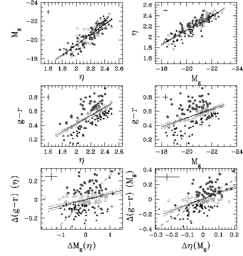
Figure 19: Correlation of $g$-band TF residuals with $g-r$ color residuals, for the forward (left) and inverse (right) relations. In the middle panels, solid lines show the best-fit mean trend of (extinction corrected) $g-r$ with $\eta$ or $M_{g}$, with dotted curves showing the bootstrap uncertainties. Filled circles, open circles, and triangles show the reddest, intermediate, and bluest 1/3 of the galaxies relative to these mean relations; the same point types are used for each galaxy in the upper and lower panels. Bottom panels plot residual from the mean color relation against TF residual. Solid and dotted lines show the best-fit residual correlation and $1\sigma$ uncertainties. Dashed lines show the expected slope for pure self-gravitating disks with mass-to-light ratio as a function of color according to Bell et al. (2003). Error crosses in each panel show median values of the observational errors.

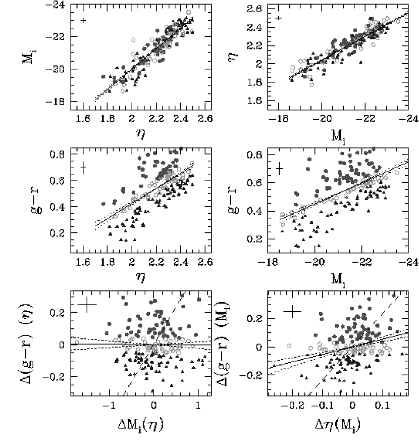
Figure 20: Correlation of $i$-band TF residual with residual from the mean relation between $i$-band half-light radius $R_{i}$ and $M_{i}$ or $\eta$. Format is similar to Fig. 19.

The top panels of Figure 19 show the forward and inverse $g$-band TF relations. The middle panels show the correlation of the extinction corrected $g$-$r$ color with $\eta$ and $M_{\lambda}$. The lines show the maximum likelihood best-fit relations, with parameters and bootstrap uncertainties listed in Table 5. Point types encode the residual color relative to this mean relation, with filled circles, open circles, and triangles showing the reddest, intermediate, and bluest 1/3 of the galaxies. The same point type is used for each galaxy in the upper panels, and one can see that red galaxies tend to be slightly underluminous in the forward relation. The top right panel of Figure 19 clearly shows that red galaxies tend to rotate faster at fixed $M_{g}$. The bottom panels plot the residual from the TF relation against the residual from the color-$\eta$ or color-$M_{g}$ relations; solid lines show the maximum likelihood fit to the mean correlation of residuals, and dotted lines show bootstrap uncertainties. The residuals are correlated, again more clearly for the inverse relation, but there is substantial scatter that is large compared to the observational errors. Note that while the bootstrap errors on the best-fit linear slopes are small, the data are not well described by any linear relation with zero intrinsic scatter, and the derived slopes therefore depend significantly on the fitting procedure. Figure 20 shows similar results for the $i$-band TF relation. The correlations between color and $i$-band TF residuals are much weaker, being essentially absent in the forward relation.

In the population synthesis modeling of Bell et al. (2003), the mass-to-light ratio of a stellar population changes with $g$-$r$ color roughly as $M_{*}/L_{g}$ $\propto$ $(g-r)^{1.52}$ in the $g$-band, and $M_{*}/L_{i}$ $\propto$ $(g-r)^{0.86}$ in the $i$-band. For pure self-gravitating disks, the circular velocity should correlate with the stellar mass as $V^{2}$ $\propto$ $M_{*}$ at fixed scale length. Variations of the stellar mass-to-light ratio would therefore produce inverse TF residual correlations of the form $\Delta(g-r)$ $\simeq$ 2$\Delta\eta(M_{g})/1.52$ and $\Delta(g-r)$ $\simeq$ 2$\Delta\eta(M_{i})/0.86$, and forward TF residuals of the form $\Delta(g-r)$ $\simeq$ $-0.4\Delta M_{g}(\eta)/1.52$ and $\Delta(g-r)$ $\simeq$ $-0.4\Delta M_{i}(\eta)/0.86$, in the absence of other effects. Dashed lines in Figure 19 and Figure 20 show the correlation slopes predicted by this simplistic model.

The residual correlations in the bottom panels of Figure 19 and Figure 20 have the correct sign expected for variations of $M_{*}/L$ with stellar populations. Therefore, we concur with the conclusion of K02 based on the NFGS, that these variations account for some of the scatter in the TF relation. However, it is clear from the scatter about the mean residual correlation, especially in the $i$-band, that these variations do not account for much of the intrinsic scatter. We have tried the experiment of changing $\eta$ for each galaxy by an amount $-\Delta\eta$ predicted from its $g$-$r$ color using the best-fit slope to the inverse TF residual correlations from Figure 19 and Figure 20, then refitting the TF relation. This procedure reduces the estimated intrinsic scatter of the inverse relation from $\sigma^{\prime}$ $=$ 0.073 to 0.057 in the $g$-band and from $\sigma^{\prime}$ $=$ 0.061 to 0.057 in the $i$-band, drops of 22% and 7%, respectively.

We can also explore the correlations of TF residuals with structural parameters. Figure LABEL:fig:radres presents the correlation of TF residuals with $i$-band half-light radius $R_{i}$, determined from the GALFIT model fits to the $i$-band images, in the same format as Figure 19 and Figure 20. In the forward relation, there is a slight tendency for larger disks at fixed $\eta$ to be slightly more luminous (upper left panel). This trend leads to a weak correlation between the TF residual and the residual from the mean $R_{i}$-$\eta$ relation, though the scatter is large compared to the mean correlation (and to the observational errors). The inverse fits reveal no trend of residual $V_{\rm 80}$ with residual $R_{i}$ at fixed $M_{i}$. Dashed lines show the predictions of a pure self-gravitating disk model, with $V^{2}$ $\propto$ 1/$R_{i}$ at fixed $M_{i}$.

These weak or absent residual-radius correlations confirm the results of Courteau & Rix (1999), now with a more broadly selected sample and smaller observational errors per galaxy. We found similar results for a disk-dominated subset in P05, using $V_{2.2}$ as a rotation measure. For the full sample, we have also investigated using the velocity at radii containing 60% to 90% of the total $i$-band flux, again with similar results. As discussed by Courteau & Rix (1999), and in greater detail by Dutton et al. (2007) and Gnedin et al. (2006), the absence of strong radius residuals imposes strong constraints on the contribution of disk gravity to the rotation speed; disk gravity should cause more compact galaxies to rotate faster, and the impact of the disk on the inner halo profile (Blumenthal et al., 1986; Gnedin et al., 2004) should amplify this effect. Explaining the observed lack of correlation requires “sub-maximal” disks, and it is more easily accomplished if disks do not produce adiabatic contraction of halos (see Dutton et al. 2007; Courteau & Rix 1999; Gnedin et al. 2006).

Figure 22 examines the dependence of the TF residuals on morphology, as quantified by the concentration index $c_{i}$ $=$ $R_{90}/R_{50}$, where $R_{90}$ and $R_{50}$ are the radii enclosing 90% and 50% of the $i$-band Petrosian flux, as determined by the SDSS photometric pipelines . An index of $c$ $\sim$ 2.6 is often adopted as the separation between early-type (high concentration) and late-type galaxies (e.g., Strateva et al. 2001). We plot early-type and late-type galaxies as filled and open circles in the top panels of Figure 22, using the $c_{i}$ $=$ 2.6 division, and the bottom panels plot $c_{i}$ against the TF residuals. On average, early-type galaxies tend to be fainter at fixed $\eta$ or rotating faster at fixed $M_{i}$, though the mean offset is small compared to the scatter. The mean residuals for early-type galaxies are $<\Delta M_{i}>$ $=$ 0.14$\pm$0.09 and $<\Delta\eta>$ $=$ 0.026$\pm$0.015, rising to 0.19$\pm$0.08 and 0.034$\pm$0.012 if we exclude the single strong outlier (J021941.13-001520.4) discussed in §5.3. This trend agrees with the finding by K02 that Sa galaxies are fainter than later type spirals at fixed rotation speed ( see also G97 and Masters et. al. (2006)). The sign of the observed trend agrees with expectations from older, redder stellar populations of early-type galaxies. However the separation in Figure 22, while modest, appears somewhat clearer than the trend with color seen in Figure 20, suggesting a direct correlation of rotation speed with morphological structure. Using the GALFIT D/T ratio, instead of $c_{i}$, gives similar results.

7 Conclusion

We have measured the TF relation for a sample of 162 galaxies selected from the SDSS, using follow-up spectroscopy to obtain H$\alpha$ rotation curves. We targeted 234 galaxies from the SDSS spectroscopic galaxy catalog that have a roughly flat absolute magnitude distribution in the range $-18.5>M_{r}>-22$. For the purpose of testing galaxy formation models, our sample has several advantages relative to most previous TF studies. Our target selection is blind to morphology, except for an $i$-band axis ratio cut of 0.6. Our completeness is high, and the galaxies with usable H$\alpha$ rotation curves have distributions of color and concentration similar to a large control sample of galaxies selected from DR4 with the same $M_{r}$ distribution but no inclination cut or H$\alpha$ requirement. Due to the uniform SDSS photometry and the selection of galaxies at redshifts greater than 5000 $\,{\rm km}\,{\rm s}^{-1}$, all sources of observational error are small compared to the estimated intrinsic scatter. The uniform multi-wavelength SDSS photometry allows us to investigate the TF relations and the correlations between TF residuals, color residuals, and other structural parameters in the $g$, $r$, $i$, and $z$-bands with minimal photometric uncertainties.

We adopt $V_{\rm 80}$ as a measure of the rotation speed and use extinction corrected absolute magnitudes. We estimate the slope, intercept, and intrinsic scatter of the TF relations simultaneously, using a maximum likelihood procedure that accounts for individual observational errors in absolute magnitude and rotation speed. We measure forward TF slopes between $-5.5$ and $-6.6\,{\rm mag}/{\rm log_{10}}(\,{\rm km}\,{\rm s}^{-1})$, with typical uncertainty of 0.2, and intercepts between $-20.7$ and $-21.5$ mag at $\eta=2.22$, with typical uncertainty of 0.04. The slope becomes systematically steeper with wavelength. Inverse fits always yield steeper slopes, but once the effects of Gaussian scatter are included, the forward and inverse fits describe essentially the same two-dimensional distribution of data points over the range covered by our data. Corrections to these slopes due to Malmquist-type biases are discussed in Appendix B, where it is shown that our observed TF relation can be reproduced with a steeper slope and larger intrinsic scatter given certain assumptions about selection effects.

The intrinsic scatter appears to be nearly independent of wavelength or fitting procedure, typically $\sigma=0.42-0.46$ mag, with a higher value (0.54 mag) for the inverse fit in $g$-band. The distribution of residuals is approximately Gaussian for both the forward and inverse relations, and there is no indication of rare outliers inflating the TF scatter, with the possible exception of one galaxy whose axis ratio may be incorrectly measured because of spiral arms. Omitting this one system reduces the estimated intrinsic scatter by 0.02 mag. The intrinsic scatter is slightly smaller for a disk-dominated subset of galaxies, decreasing in the $i$-band from 0.42 mag to 0.36 mag for galaxies having disk-to-total flux ratios greater than 0.9. Morphologically asymmetric, barred, or possibly interacting galaxies show no clear evidence for offsets from the mean TF relation or for larger scatter, though our statistics for these subsets are limited.

In an attempt to understand the origin of scatter in the TF relation, we study correlations between TF residuals and other galaxy properties: $g-r$ color, half-light radius, and $i$-band concentration index. The $g$-band TF residual shows a significant correlation with color, in the sense that bluer galaxies are brighter at fixed $\eta$ or (more clearly visible in the data) that redder galaxies rotate faster at fixed $M_{g}$. However, these correlations are much weaker in the $i$-band, and they are much weaker than predicted for pure self-gravitating disks with the stellar mass-to-light ratios predicted from $g-r$ color. The correlation with half-light radius is very weak, with a slight tendency for larger galaxies to be more luminous at fixed $\eta$. More concentrated (earlier type) galaxies tend to be slightly fainter at fixed $\eta$ or to rotate slightly faster at fixed $M_{i}$, but the trend is weak compared to the TF scatter.

Our TF relation is similar to that found for field spirals by C97, who used similar analysis methods. The TF relation found by V01 for Ursa Major spirals, using the flat portion of HI rotation curves as a velocity measure, is significantly steeper than ours. This difference may partly reflect the difference in velocity width definitions, and Malmquist-type biases as described in Appendix B. The residual correlations in our sample are similar to those found by K02 using the Nearby Field Galaxy Survey of Jansen et al. (2000), but we find that stellar population effects explain only a small fraction of the scatter in the TF relation.

The nearly constant intrinsic scatter of the TF relation has interesting implications for galaxy formation theories. The scatter is only slightly larger in bluer bands and only slightly smaller for a morphologically selected disk-dominated sub-sample of galaxies, and the correlation of TF residuals with other properties explains only a small fraction of the scatter. The lack of correlation with radius implies that disk gravity has small influence on galaxy dynamics at the radii used for TF measurements; this observational result provides a strong constraint on galaxy formation models (Dutton et al., 2007; Gnedin et al., 2006). The weak correlation with color, size, and morphology implies that most of the scatter in the TF relation arises from genuine variation in the ratio of dark matter to baryonic matter from halo to halo.

Our results suggest many fruitful directions for future observational investigations, each of them comparable in magnitude to the one undertaken here. Absorption-line velocity measurements, which require longer exposures than our H$\alpha$ emission line measurements, could yield rotation velocities for the remaining 30% of our sample, showing whether galaxies without H$\alpha$ emission follow a systematically different TF relation. HI measurements would allow detailed comparison between TF relations defined by H$\alpha$ and HI velocity widths (see C97) for our broadly selected galaxy sample, and they would provide gas masses and gas fractions as additional parameters for residual correlation studies, which would be valuable for testing theoretical models (Dutton et al., 2007; Gnedin et al., 2006). Extending the TF relation to brighter and fainter luminosities is of great interest (e.g., McGaugh et al. 2000), though complications arise from the growing paucity of disks in the first case and the increasing importance of non-circular motions in the second. Finally, it is clear that detailed investigation of TF residuals would benefit from a much larger sample with similarly broad selection criteria and similarly small observational errors, so that one could, for example, investigate residual correlations with size, morphology, or environment within restricted regions of luminosity-color space. Since large samples of galaxies ($\geq 2000$) have been observed for TF studies in the past (see, e.g., Courteau et al. 2003; Masters et. al. 2006 and references therein), it may be possible to construct such a sample largely from archival data, if the data quality can be made sufficiently homogeneous and the effects of sample selection can be sufficiently well understood. Our data already provide a well defined and highly constraining target for theoretical models of galaxy formation. Extended observational studies would improve our ability to deduce the essential physics of disk galaxy formation empirically.

Appendix A TF Parameters for Alternative Parameters and Sample Cuts

Our standard TF fits, presented in Table 4, use all flag-1,2,3 galaxies, absolute magnitudes corrected for internal extinction, velocities defined by $V_{\rm 80}$, and equal contribution of each galaxy to the likelihood sums of equation (14). Table 6 presents TF fits using a number of variations on parameter definitions and sample cuts or weights. First, we list results for the full sample with the usual definitions but weights chosen to approximate a truly flat absolute magnitude distribution in the range $-18.5>M_{r}>-22$ (see §5.2). Next, we list results for the full sample with the usual weights but no internal extinction correction (see Fig. 12). Then we list results for two alternative velocity width definitions: the value of the arc-tangent functional fit evaluated at 2.2 disk scale lengths as determined from the $i$-band GALFIT model ($V_{2.2}$), and at the location of the most distant H$\alpha$ data point ($V_{end}$). Finally, we list the TF fits for the standard definitions and flag-1,2 galaxies only. Although slopes and intercepts change somewhat with these choices, none of our conclusions about the TF relation would be qualitatively different for any of these alternative choices.

Appendix B Malmquist-type Biases in Our TF Sample.

Applying magnitude cuts to TF samples can lead to biased estimates of the TF parameters because there are low and high luminosity galaxies, at fixed velocity, scattered above or below the magnitude limits. This can be due to both the intrinsic scatter and peculiar velocities scattering galaxies across selection boundaries. Most discussions of these “Malmquist”-type biases have focused on apparent magnitude limited samples, or on the systematic bias in the derived peculiar velocity field (e.g., Lynden-Bell et al. 1988; Gould 1993; Teerikorpi 1993; Strauss & Willick 1995). Since our selection procedure is quite different from those of most previous TF surveys, we have tested for Malmquist-type biases with a simple Monte Carlo experiment.

We first investigate the affect our absolute magnitude-redshift cuts and flag-1,2,3 absolute magnitude distribution will have on our measured TF relation. For our Monte Carlo experiment, we generate a sample of $10^{5}$ galaxies, evenly sampled in logarithmic velocity space, assigning random positions in a space between 4000 $\,{\rm km}\,{\rm s}^{-1}$ and 16000 $\,{\rm km}\,{\rm s}^{-1}$. We then assign absolute magnitudes to each galaxy following an assumed TF relation, having a Gaussian intrinsic scatter, represented by

$$M=a_{ub}(\eta-\eta_{0})+b_{ub}+N(0,\sigma_{ub}),$$ (B1)

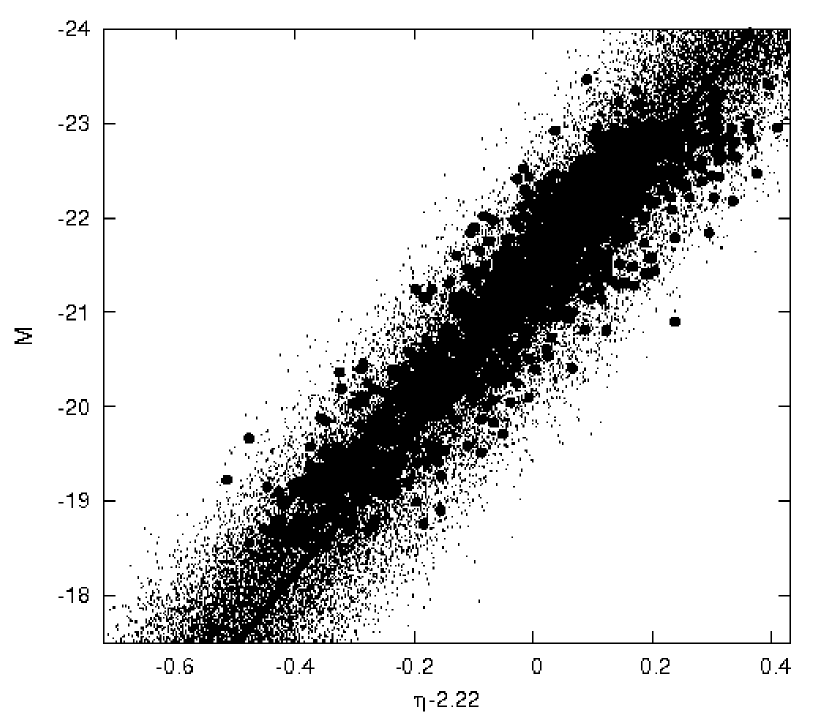
Figure 23: A Monte Carlo sample without absolute magnitude cuts (small dots) and with our absolute magnitude cuts applied (filled circles). The relation used to generate the sample is shown as a solid line, the dotted line is the best-fit to the sample after the cuts have been applied.

where $a_{ub}$, $b_{ub}$, and $\sigma_{ub}$ are the slope, intercept, and intrinsic scatter for an un-biased power-law TF relation. We use $\eta_{0}=2.22$ throughout the procedure. We then apply our absolute magnitude-redshift cuts, outlined in §2, and select galaxies according to our observed flag-1,2,3 absolute magnitude distribution, with a final Monte Carlo sample that is 10 times larger than our flag-1,2,3 sample, or 1620 galaxies. Generating a Monte Carlo sample with $a_{ub}$ $=$ -7.52, $b_{ub}$ $=$ -21.23, and $\sigma_{ub}$ $=$ 0.45, and applying our cuts, will have a measured TF relation with a slope, intercept, and scatter of -6.86, -21.27, 0.33. This is quite a large difference considering our typical statistical uncertainties on the measure slope, intercept, and scatter being 0.2, 0.04, and 0.04 mag respectively. The effect on the inverse relation is much smaller since the cuts are applied to absolute magnitudes. Figure 23 shows this Monte Carlo sample with and without these cuts. It is clear from Figure 23 that the selection criteria has excluded high and low luminosity galaxies, shallowing the slope and reducing the scatter.

The measurement errors in SDSS Petrosian magnitudes are generally small, and luminosity uncertainties are therefore dominated by line-of-sight peculiar velocities, which we have assumed in our analysis to be drawn from a Gaussian of dispersion $300\,{\rm km}\,{\rm s}^{-1}$. Next we include peculiar velocities in the Monte Carlo sample by modifying each galaxy’s redshift with a peculiar velocity drawn from a $300\,{\rm km}\,{\rm s}^{-1}$ Gaussian. We then apply the same absolute-magnitude redshift cuts, while matching the flag-1,2,3 absolute magnitude distribution in the shaded area of Figure 1, then measure the TF relation for this sample. Generating a Monte Carlo sample with $a_{ub}$ $=$ -7.52, $b_{ub}$ $=$ -21.23, and $\sigma_{ub}$ $=$ 0.45 has a measured slope $=$ -6.77, intercept $=$ -21.34, and $\sigma$ $=$ 0.33 mag. This is a relatively small, but non-zero, effect. We include the 300$\,{\rm km}\,{\rm s}^{-1}$ peculiar velocities in the analysis below.

We now estimate what power-law TF relation and Gaussian intrinsic scatter would be required to reproduce the measured forward TF relations in Table 4, given our selection criteria. This is done iteratively by varying $a_{ub}$, $b_{ub}$, and $\sigma_{ub}$, until the fitted parameters, after applying our selection criteria and 300$\,{\rm km}\,{\rm s}^{-1}$ peculiar velocities, agree with the measure TF relations reported in Table 4. The forward $i$-band TF relation in Table 4 is reproduced with un-biased values of $a_{ub}$ $=$ -7.35, $b_{ub}$ $=$ -21.27, and $\sigma_{ub}$ $=$ 0.58 mag. Comparing these numbers to the best-fit values for the forward $i$-band relation in Table 4, shows that the un-biased slope is steeper by $\sim$ 5 sigma, the intercept changed by several sigma, and the un-biased intrinsic scatter is larger by $\sim$ 4-5 sigma. Similar results are found for the $g$, $r$, and $z$-bands. The un-biased $r$-band TF parameters, that reproduce the best-fit values in Table 4, are $a_{ub}$ $=$ -7.02, $b_{ub}$ $=$ -21.05, and $\sigma_{ub}$ $=$ 0.56 mag.

Table 4 presents the best-fit TF relation to galaxies observed with the selection criteria outlined in §2. Although the un-biased parameters discussed here are quite different from the best-fit TF parameters, the best-fit parameters have fewer assumptions than the un-biased parameters and have well defined selection criteria. Namely, the un-biased power-law TF relation assumes that there is no change in slope at high and low luminosities (contrary to K02), and that the best-fit TF parameters in Table 4 are a fit to the data and not a Monte Carlo experiment. However, G97 show that these assumptions have a small affect on the un-biased parameters. Therefore, the recommended procedure when trying to reproduce the TF relation in the SDSS bands would be to apply our selection criteria and absolute magnitude distributions to a sample (theoretical or observed), then measure the best-fit parameters.

Figure 1: Distribution of $r$-band absolute magnitudes for the full sample targeted for follow-up H$\alpha$ observations (234 galaxies, full histogram) and the subset of the sample with usable (flag-1,2,3) H$\alpha$ rotation curves (170 galaxies, shaded histogram)

Figure 2: The color magnitude relation for our sample of galaxies plotted on top of contours containing 25%, 50%, and 75% of the total luminosity density in the whole low redshift DR2 sample (Blanton et al., 2003b). The data point type indicates the quality of the galaxy rotation curve corresponding to flag-1 (circles), flag-2 (squares), flag-3 (asterisks), and flag-4 (diamonds).

Figure 3: Cumulative distributions of the (top) $g$-$r$ model color and (bottom) $i$-band concentration index ($r_{90}/r_{50}$) for our full sample (short-dashed curves), the subset with usable rotation curves (long-dashed curves), and “control” samples with the same $M_{r}$ distribution selected from SDSS DR4, with (dotted) and without (solid) an isophotal axis ratio cut $b/a$ $\leq$ 0.6.

Figure 5: Comparison of rotation curves measured at MDM (filled triangles) and Calar Alto (open triangles). Dotted and solid curves show the arc-tangent function fits to the MDM and Calar Alto data, respectively.

Figure 9: Major axis surface brightness profiles (averaged over five pixels in each direction) of the three galaxies shown in Figure 8. In the left panels, points show the data, solid curves show the GALFIT model, and vertical lines mark the half-light diameter. Right hand panels plot the residual counts (model$-$data); for these galaxies, 10 counts/pixel corresponds to roughly 23.4 mag/arcsec² in the $i$-band.

Figure 10: The $i$-band $D/T$ vs. the concentration index ($r_{90}/r_{50}$) for the $flag-1,2,3$ galaxies.

Figure 11: Histograms of the total internal extinction for the $g$, $r$, $i$, and $z$-bands.

Figure 13: The $i$-band TF relation for the full galaxy sample (top), flag-1,2 galaxies (middle), and flag-1 galaxies only (bottom). Solid and dotted lines show forward and inverse fits, respectively. The forward slope, intercept (at $\eta_{0}$ $=$ 2.22), and intrinsic scatter are listed as $a$, $b$, and $\sigma$, while $a^{\prime}$, $b^{\prime}$, $\sigma^{\prime}$ refer to the converted inverse fit parameters. Parameter uncertainties are listed in Tables 4 and 6. Table 4.

Figure 14: TF relations for the full (flag-1,2,3) sample in the $g$, $r$, $i$, and $z$-bands. The format is similar to Figure 13, except that we show the 10-th percentile, median, 90-th percentile 1$\sigma$ errors crosses in each panel instead of plotting errors on each data point. All intercepts $(b,b^{\prime})$ are quoted at the $\eta_{0}$ values listed in Table 4.

Figure 15: (Top) TF relation with the seven largest outliers (in terms of $\Delta\chi^{2}$) marked in rank order. (Bottom) Estimated intrinsic scatter of the $i$-band TF relation after omitting the $N_{\rm removed}$ data points with the largest $\Delta\chi^{2}$. The solid circles represent the forward TF relation and the open circles the inverse. The slope as a function of removed data points is shown in the inset.

Figure 16: Distribution of residuals for the $i$-band TF relation, with $\Delta y\equiv y-\bar{y}(x)$, $y\equiv M_{i}$ for the forward (solid histogram) relation and $y\equiv\eta$ for the inverse (dotted histogram) relation, and the total scatter for a galaxy with observational errors $\sigma_{x}$, $\sigma_{y}$ defined by $\sigma_{T}^{2}$ = $\sigma^{2}$ + $\sigma_{y}^{2}$ + $(a\sigma_{x})^{2}$. The smooth solid curve is a Gaussian of unit dispersion. The TF outlier J021941.13-001520.4 for both the forward and inverse relations is at $\Delta y$/$\sigma_{T}$ $\sim$ $-4$.

Figure 17: TF relations for morphologically identified subsamples. (Top) Filled circles represent galaxies with disk-to-total flux ratios $D/T>0.9$; open circles represent other sample galaxies. Solid and dotted lines show best-fit $i$-band TF relations for the full and disk-dominated samples, respectively. (Bottom) TF relation in $g$-band with asymmetrical, barred, and “interacting” galaxies (with nearby neighbors) marked by triangles, squares, and asterisks, respectively. The solid line is the best-fit relation for the full data set.

Figure 18: Comparison to results from C97’s field sample and V01’s sample from the Ursa Major cluster. (Top) Filled and open circles show galaxies from C97 and from this paper, respectively; dotted and solid curves show the corresponding forward TF fits. Velocities are $V_{\rm 80}$ for our points and $V_{2.2}$ for C97. (Bottom) Same as above, but with filled triangles representing the V01 data. Absolute magnitudes are SDSS $r$ for our points and Johnson $R$ for V01. Velocities for V01 are $V_{\rm flat}$, measured from the flat portion of HI synthesis rotation curves.

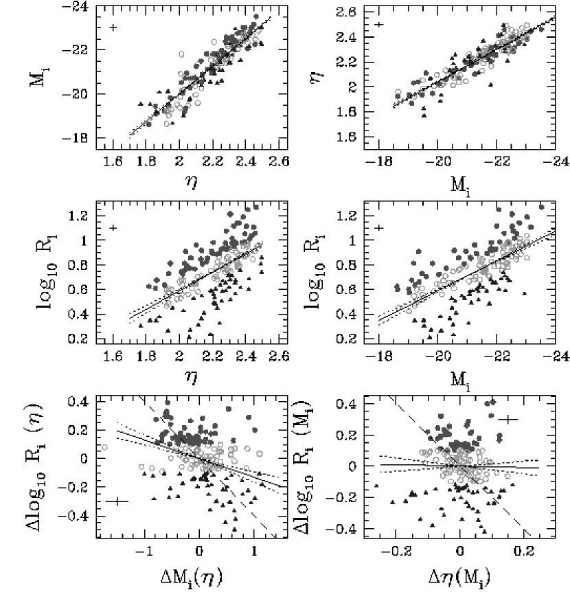
Figure 21: Correlation of $i$-band TF residualfrom the mean relation between $i$-band half-light radius $R_{i}$ and $M_{i}$ or $\eta$. The Format is otherwise the same as Figure 19.

Figure 22: Correlation of $i$-band TF residual with $i$-band concentration index $c_{i}=r_{90}/r_{50}$. Lower panels plot $c_{i}$ vs. TF residual. In all panels, filled and open circles show “early” and “late” galaxy types, respectively, with the division between types at $c_{i}=2.6$.

Table 1: Telescope and Spectrograph Parameters

Parameter	Calar Alto	MDM
Telescope	3.5 meter	2.4 meter
Spectrograph	TWIN	CCDS
Grating	1200 lines/mm	600 lines/mm
Blaze	7100 (1st order) Å	5875 (2nd order) Å
Spectral Coverage	6200-7300 Å	6500-6994 Å
Slit Width	$1.5"\times 4^{\prime}$	$2"\times 5^{\prime}$
Spatial Scale	$0.56"/$pix	$0.41"$/pix
Dispersion	0.55 Å/pix	0.41 Å/pix
Read Noise	3.9 e-	7e-
Gain	0.865 e-/ADU	2.1 e-/ADU
Detector	SITe 2000 x 800 CCD	Loral 1200x800 CCD
Net Instrument Eff.	0.2	$\sim$ 0.15

Table 2: Photometric Parameters

SDSS name	$d_{\rm lg}/{\rm Mpc}$	$M_{g}$	$M_{r}$	$M_{i}$	$M_{z}$	$g$-$r$	$D/T$	$R_{i}$/kpc	$b/a_{i}$
J001006.62-002609.6	143.75(4.39)	-21.16(0.18)	-21.30(0.15)	-21.38(0.14)	-21.22(0.09)	0.49(0.03)	0.92	3.82(0.17)	0.30(0.01)
J001708.77-005728.9	84.81(4.35)	-19.57(0.15)	-20.04(0.14)	-20.26(0.13)	-20.24(0.12)	0.48(0.03)	1.00	5.11(0.28)	0.58(0.01)
J001947.33+003526.7	79.65(4.34)	-19.24(0.13)	-19.82(0.12)	-20.12(0.12)	-20.27(0.12)	0.54(0.01)	0.54	1.83(0.10)	0.64(0.01)
J002025.78+004934.9	76.13(4.34)	-20.29(0.21)	-21.01(0.19)	-21.26(0.17)	-21.14(0.15)	0.74(0.02)	0.92	9.15(0.55)	0.41(0.01)
J003112.09-002426.4	87.00(4.35)	-20.16(0.14)	-20.87(0.14)	-21.14(0.12)	-21.33(0.12)	0.74(0.01)	0.79	3.11(0.16)	0.52(0.01)
J003629.24-004342.8	152.58(4.40)	-19.98(0.06)	-20.78(0.06)	-21.18(0.06)	-21.47(0.06)	$\cdots$	$\cdots$	$\cdots$	$\cdots$
J003856.59+001757.3	115.60(4.37)	-19.13(0.08)	-19.94(0.08)	-20.34(0.08)	-20.65(0.08)	$\cdots$	$\cdots$	$\cdots$	$\cdots$
J004239.34+001638.7	195.48(4.43)	-21.82(0.16)	-22.23(0.13)	-22.41(0.11)	-22.34(0.08)	0.60(0.03)	0.93	9.45(0.40)	0.55(0.01)
J004759.81+011209.2	194.18(4.43)	-20.93(0.09)	-21.71(0.06)	-22.14(0.06)	-22.42(0.05)	$\cdots$	$\cdots$	$\cdots$	$\cdots$
J004935.68+010655.5	78.47(4.34)	-21.32(0.49)	-21.80(0.40)	-22.00(0.33)	-21.88(0.26)	0.56(0.09)	1.00	13.08(0.75)	0.10(0.01)
J005513.63-010433.8	213.99(4.44)	-21.68(0.23)	-22.32(0.20)	-22.61(0.15)	-22.74(0.12)	0.67(0.04)	0.85	10.39(0.43)	0.30(0.01)
J005516.88-005504.5	198.00(4.43)	-20.85(0.06)	-21.64(0.06)	-22.02(0.06)	-22.30(0.06)	$\cdots$	$\cdots$	$\cdots$	$\cdots$
J005603.35-004941.0	199.28(4.43)	-20.49(0.05)	-21.32(0.05)	-21.74(0.05)	-22.03(0.05)	$\cdots$	$\cdots$	$\cdots$	$\cdots$
J005605.99+003742.0	188.38(4.42)	-20.72(0.05)	-21.52(0.05)	-21.95(0.05)	-22.19(0.05)	$\cdots$	$\cdots$	$\cdots$	$\cdots$
J005619.60-000732.7	194.18(4.43)	-20.79(0.07)	-21.64(0.07)	-22.05(0.07)	-22.34(0.06)	$\cdots$	$\cdots$	$\cdots$	$\cdots$
J005620.00-011035.9	175.00(4.41)	-20.42(0.06)	-21.31(0.06)	-21.75(0.06)	-22.03(0.06)	$\cdots$	$\cdots$	$\cdots$	$\cdots$
J005624.61-010834.9	193.23(4.42)	-20.49(0.05)	-21.25(0.05)	-21.63(0.05)	-21.88(0.05)	$\cdots$	$\cdots$	$\cdots$	$\cdots$
J005650.61+002047.1	188.75(4.42)	-21.34(0.11)	-22.06(0.10)	-22.32(0.06)	-22.54(0.06)	0.73(0.01)	0.29	6.39(0.25)	0.33(0.01)
J010338.82-002927.9	77.90(4.34)	-18.74(0.12)	-19.17(0.14)	-19.39(0.12)	-19.17(0.14)	$\cdots$	$\cdots$	$\cdots$	$\cdots$
J010823.24+000523.1	210.48(4.44)	-21.05(0.05)	-21.91(0.05)	-22.34(0.05)	-22.65(0.05)	$\cdots$	$\cdots$	$\cdots$	$\cdots$
J011341.82-000609.9	76.96(4.34)	-20.48(0.18)	-21.10(0.16)	-21.39(0.14)	-21.51(0.13)	0.63(0.04)	0.69	4.12(0.24)	0.46(0.01)
J011446.94+003128.9	203.46(4.43)	-20.47(0.06)	-21.36(0.06)	-21.78(0.06)	-22.09(0.06)	$\cdots$	$\cdots$	$\cdots$	$\cdots$
J011508.73+003433.6	203.31(4.43)	-20.53(0.05)	-21.42(0.06)	-21.85(0.05)	-22.17(0.05)	$\cdots$	$\cdots$	$\cdots$	$\cdots$
J011520.86+001533.5	194.16(4.43)	-21.20(0.12)	-21.79(0.10)	-22.09(0.08)	-22.24(0.06)	0.66(0.03)	0.44	9.68(0.48)	0.26(0.01)
J011605.60-000053.6	199.98(4.43)	-21.25(0.05)	-22.15(0.07)	-22.63(0.08)	-22.96(0.09)	0.93(0.04)	0.88	8.89(0.45)	0.31(0.01)
J012000.48-002826.9	200.46(4.43)	-21.27(0.11)	-21.90(0.09)	-22.22(0.08)	-22.38(0.07)	0.76(0.02)	0.69	6.19(0.16)	0.54(0.02)
J012223.78-005230.7	120.89(4.37)	-22.80(0.27)	-23.28(0.21)	-23.52(0.16)	-23.46(0.13)	0.67(0.06)	0.90	18.56(0.79)	0.45(0.01)
J012312.37-003828.2	122.67(4.37)	-20.63(0.08)	-21.50(0.08)	-21.93(0.09)	-22.22(0.08)	$\cdots$	$\cdots$	$\cdots$	$\cdots$
J012317.00-005421.7	115.16(4.37)	-20.70(0.22)	-21.28(0.21)	-21.43(0.14)	-21.54(0.12)	0.64(0.02)	0.79	4.33(0.18)	0.28(0.01)
J012340.13+004056.5	148.43(4.39)	-21.21(0.33)	-21.55(0.24)	-21.63(0.15)	-21.73(0.11)	0.41(0.10)	0.72	5.90(0.23)	0.17(0.01)
J012438.08-000346.4	123.50(4.37)	-20.81(0.31)	-21.22(0.21)	-21.48(0.17)	-21.57(0.13)	0.45(0.10)	0.78	6.69(0.29)	0.18(0.01)
J012859.57-003342.9	81.38(4.34)	-20.85(0.12)	-21.65(0.12)	-22.04(0.12)	-22.27(0.12)	$\cdots$	$\cdots$	$\cdots$	$\cdots$
J013142.14-005559.9	80.66(4.34)	-21.84(0.32)	-22.50(0.27)	-22.76(0.22)	-22.93(0.18)	0.71(0.06)	0.70	13.90(0.76)	0.15(0.01)
J013600.15+003948.6	77.10(4.34)	-21.07(0.15)	-21.71(0.16)	-21.92(0.14)	-21.83(0.13)	0.73(0.01)	0.84	6.15(0.36)	0.58(0.01)
J013752.69+010234.8	196.07(4.43)	-21.67(0.27)	-22.24(0.20)	-22.50(0.16)	-22.67(0.12)	0.61(0.07)	0.77	8.18(0.34)	0.23(0.01)
J014121.94+002215.7	135.13(4.38)	-20.49(0.15)	-21.08(0.12)	-21.38(0.10)	-21.59(0.09)	0.65(0.03)	0.72	3.27(0.13)	0.43(0.01)
J015550.32+004319.2	208.12(4.44)	-20.82(0.05)	-21.65(0.05)	-22.07(0.05)	-22.35(0.05)	$\cdots$	$\cdots$	$\cdots$	$\cdots$
J015746.24-011229.9	187.72(4.42)	-22.22(0.35)	-22.80(0.28)	-23.02(0.23)	-23.12(0.17)	0.64(0.07)	0.93	7.19(0.32)	0.21(0.01)
J015840.93+003145.2	103.78(4.36)	-21.79(0.21)	-22.21(0.18)	-22.39(0.14)	-22.24(0.12)	0.54(0.04)	0.89	9.46(0.46)	0.46(0.01)
J015852.30+003405.9	103.57(4.36)	-19.73(0.09)	-20.57(0.09)	-20.98(0.09)	-21.24(0.09)	$\cdots$	$\cdots$	$\cdots$	$\cdots$
J015946.76-001657.7	194.89(4.43)	-21.65(0.18)	-22.17(0.15)	-22.37(0.12)	-22.41(0.09)	0.58(0.04)	0.95	7.63(0.38)	0.49(0.01)
J020004.87-001644.8	123.49(4.37)	-20.79(0.25)	-21.22(0.19)	-21.44(0.16)	-21.52(0.13)	0.54(0.06)	0.90	5.70(0.26)	0.28(0.01)
J020045.13-101451.3	81.75(4.34)	-18.25(0.14)	-18.58(0.13)	-18.64(0.13)	-18.63(0.14)	0.37(0.02)	1.00	3.97(0.21)	0.54(0.01)
J020158.20-005951.9	192.44(4.42)	-20.56(0.07)	-21.41(0.07)	-21.81(0.07)	-22.11(0.07)	$\cdots$	$\cdots$	$\cdots$	$\cdots$
J020447.19+005006.3	88.98(4.35)	-18.93(0.23)	-19.14(0.18)	-19.19(0.15)	-19.24(0.13)	0.27(0.06)	1.00	3.52(0.18)	0.26(0.01)
J020540.31-004141.4	189.64(4.42)	-21.62(0.17)	-22.18(0.14)	-22.52(0.10)	-22.66(0.08)	0.71(0.04)	0.84	16.34(0.70)	0.15(0.01)
J020621.28-085218.0	79.61(4.34)	-18.61(0.12)	-18.77(0.12)	-18.77(0.12)	-17.94(0.12)	$\cdots$	$\cdots$	$\cdots$	$\cdots$
J020853.01+004712.6	188.47(4.42)	-21.96(0.19)	-22.49(0.15)	-22.78(0.12)	-22.82(0.10)	0.57(0.04)	0.98	9.58(0.43)	0.51(0.01)
J021112.60-004933.1	182.41(4.42)	-21.67(0.13)	-22.11(0.08)	-22.36(0.06)	-22.46(0.06)	0.52(0.05)	0.37	6.09(0.23)	0.51(0.01)
J021159.96+011302.8	103.24(4.36)	-19.47(0.22)	-18.42(0.48)	-18.12(0.52)	-18.51(0.70)	$\cdots$	$\cdots$	$\cdots$	$\cdots$
J021219.68-004841.4	181.93(4.42)	-21.48(0.05)	-22.29(0.05)	-22.76(0.05)	-23.02(0.05)	$\cdots$	$\cdots$	$\cdots$	$\cdots$
J021859.65+001948.0	132.52(4.38)	-20.97(0.23)	-21.47(0.19)	-21.71(0.16)	-21.81(0.12)	0.59(0.04)	0.98	5.14(0.23)	0.36(0.01)
J021941.13-001520.4	114.33(4.37)	-21.22(0.15)	-21.65(0.14)	-21.81(0.12)	-21.76(0.10)	0.45(0.03)	0.68	4.77(0.21)	0.51(0.01)
J022026.54-001846.3	185.33(4.42)	-21.08(0.05)	-21.95(0.05)	-22.35(0.05)	-22.65(0.05)	$\cdots$	$\cdots$	$\cdots$	$\cdots$
J022606.71-001954.9	94.38(4.35)	-22.00(0.24)	-22.47(0.19)	-22.69(0.16)	-22.65(0.14)	0.55(0.05)	0.97	11.28(0.57)	0.48(0.01)
J022751.44+003005.5	182.35(4.42)	-22.54(0.41)	-22.89(0.31)	-23.03(0.24)	-23.00(0.18)	0.49(0.10)	0.93	15.50(0.65)	0.21(0.01)
J022820.86+004114.0	183.32(4.42)	-21.58(0.14)	-21.99(0.11)	-22.20(0.09)	-22.18(0.08)	0.48(0.03)	0.94	6.79(0.33)	0.61(0.01)
J023240.17+001536.4	90.98(4.35)	-20.84(0.10)	-21.61(0.10)	-22.00(0.10)	-22.20(0.10)	$\cdots$	$\cdots$	$\cdots$	$\cdots$
J023301.24+002515.0	99.49(4.36)	-20.86(0.12)	-21.39(0.11)	-21.66(0.10)	-21.78(0.10)	0.56(0.02)	0.46	3.87(0.18)	0.55(0.01)
J023437.74-005847.3	220.20(4.44)	-21.74(0.19)	-22.54(0.21)	-22.52(0.09)	-22.72(0.07)	0.84(0.02)	0.36	12.97(0.43)	0.18(0.01)
J023522.55-000700.4	220.55(4.44)	-21.07(0.04)	-21.87(0.04)	-22.24(0.04)	-22.53(0.04)	$\cdots$	$\cdots$	$\cdots$	$\cdots$
J023610.91-005833.8	220.05(4.44)	-22.14(0.28)	-22.65(0.22)	-22.89(0.18)	-23.01(0.13)	0.57(0.06)	0.94	9.18(0.41)	0.32(0.01)
J023915.02+002842.5	217.21(4.44)	-20.69(0.05)	-21.56(0.05)	-21.99(0.05)	-22.30(0.05)	$\cdots$	$\cdots$	$\cdots$	$\cdots$
J024331.30+001824.5	118.21(4.37)	-22.27(0.26)	-22.79(0.21)	-23.03(0.16)	-23.02(0.13)	0.56(0.06)	0.82	9.72(0.42)	0.35(0.01)
J024436.70+000831.5	125.38(4.38)	-19.52(0.08)	-20.29(0.08)	-20.67(0.08)	-20.93(0.08)	$\cdots$	$\cdots$	$\cdots$	$\cdots$
J024459.89+010318.5	112.33(4.37)	-20.82(0.29)	-21.32(0.24)	-21.54(0.20)	-21.66(0.15)	0.55(0.05)	0.99	5.53(0.26)	0.25(0.01)
J024527.56+005451.6	107.87(4.36)	-21.48(0.18)	-21.99(0.12)	-22.24(0.09)	-22.46(0.09)	0.57(0.08)	0.09	5.48(0.26)	0.26(0.01)
J024558.37-002657.1	128.40(4.38)	-19.95(0.07)	-20.79(0.07)	-21.20(0.07)	-21.45(0.07)	$\cdots$	$\cdots$	$\cdots$	$\cdots$
J024727.83-001706.4	94.80(4.35)	-21.53(0.11)	-22.13(0.11)	-22.43(0.11)	-22.43(0.11)	0.74(0.01)	0.71	4.68(0.24)	0.68(0.01)
J024728.01+003906.9	199.09(4.43)	-21.34(0.17)	-22.00(0.16)	-22.28(0.13)	-22.47(0.10)	0.65(0.01)	0.92	5.12(0.26)	0.38(0.01)
J024744.89+002451.0	123.49(4.37)	-21.36(0.20)	-21.89(0.18)	-21.79(0.08)	-21.75(0.09)	0.69(0.02)	0.19	8.46(0.60)	0.46(0.01)
J024850.79-004602.6	95.50(4.35)	-21.59(0.25)	-22.15(0.21)	-22.37(0.17)	-22.39(0.14)	0.63(0.05)	0.92	6.51(0.32)	0.37(0.01)
J024935.34-004325.5	96.82(4.36)	-19.87(0.17)	-20.11(0.13)	-20.14(0.11)	-20.17(0.10)	0.28(0.05)	0.37	3.64(0.17)	0.20(0.01)
J024949.33-004736.6	198.68(4.43)	-21.57(0.20)	-22.10(0.15)	-22.38(0.12)	-22.54(0.09)	0.60(0.05)	0.77	7.56(0.34)	0.35(0.01)
J025154.59+003953.3	129.61(4.38)	-21.02(0.13)	-21.75(0.16)	-21.83(0.09)	-21.83(0.08)	0.81(0.04)	0.37	8.31(0.34)	0.31(0.01)
J025338.43+011212.2	142.91(4.39)	-19.53(0.07)	-20.39(0.07)	-20.81(0.07)	-21.14(0.07)	$\cdots$	$\cdots$	$\cdots$	$\cdots$
J025627.12+005232.6	101.39(4.36)	-21.27(0.17)	-21.65(0.13)	-21.81(0.12)	-21.64(0.11)	0.44(0.05)	0.99	9.59(0.45)	0.64(0.01)
J025640.44-005614.2	192.64(4.42)	-20.37(0.06)	-21.22(0.06)	-21.63(0.06)	-21.93(0.06)	$\cdots$	$\cdots$	$\cdots$	$\cdots$
J030540.35-002406.9	109.35(4.36)	-18.06(0.09)	-18.80(0.09)	-19.11(0.09)	-19.35(0.09)	$\cdots$	$\cdots$	$\cdots$	$\cdots$
J032019.21+003005.4	103.19(4.36)	-18.36(0.12)	-18.64(0.11)	-18.66(0.10)	-18.80(0.11)	0.30(0.03)	1.00	2.83(0.12)	0.53(0.01)
J032251.25+000822.7	101.62(4.36)	-17.54(0.10)	-18.24(0.15)	-18.57(0.10)	-18.88(0.11)	$\cdots$	$\cdots$	$\cdots$	$\cdots$
J032257.99+000314.9	157.92(4.40)	-20.77(0.22)	-21.32(0.18)	-21.61(0.14)	-21.70(0.11)	0.61(0.04)	0.84	5.62(0.19)	0.24(0.01)
J033329.46-073308.4	76.72(4.34)	-19.11(0.20)	-19.45(0.17)	-19.48(0.15)	-19.41(0.15)	0.35(0.03)	1.00	3.63(0.21)	0.36(0.01)
J033331.54+004157.4	161.64(4.40)	-21.57(0.27)	-22.10(0.23)	-22.33(0.16)	-22.51(0.13)	0.62(0.08)	0.48	9.31(0.30)	0.12(0.01)
J033607.78-003547.2	103.12(4.36)	-20.10(0.13)	-20.70(0.11)	-21.04(0.10)	-21.30(0.10)	0.62(0.04)	0.40	2.11(0.09)	0.34(0.01)
J035356.55-070422.6	145.95(4.39)	-20.85(0.07)	-21.80(0.07)	-22.26(0.07)	-22.60(0.07)	$\cdots$	$\cdots$	$\cdots$	$\cdots$
J080046.85+353146.0	76.40(4.34)	-18.55(0.16)	-18.87(0.14)	-19.01(0.14)	-18.98(0.13)	0.37(0.02)	1.00	2.67(0.16)	0.49(0.01)
J080126.42+441137.0	138.77(4.39)	-21.63(0.26)	-22.19(0.21)	-22.50(0.16)	-22.66(0.13)	0.60(0.06)	0.88	7.41(0.30)	0.31(0.01)
J080658.75+463346.8	97.38(4.36)	-20.47(0.33)	-21.08(0.27)	-21.41(0.22)	-21.53(0.18)	0.65(0.06)	0.96	6.27(0.30)	0.16(0.01)
J080927.22+435605.6	100.83(4.36)	-20.23(0.18)	-20.79(0.15)	-21.05(0.13)	-21.21(0.11)	0.68(0.04)	0.79	4.64(0.21)	0.38(0.01)
J081313.84+402504.6	114.66(4.37)	-17.29(0.10)	-18.09(0.09)	-18.40(0.11)	-17.80(0.13)	$\cdots$	$\cdots$	$\cdots$	$\cdots$
J082949.87+484647.9	105.70(4.36)	-21.14(0.32)	-21.58(0.26)	-21.82(0.21)	-21.76(0.16)	0.58(0.07)	1.00	6.70(0.31)	0.27(0.01)
J082956.27+515824.1	77.15(4.34)	-19.26(0.21)	-19.46(0.18)	-19.48(0.16)	-19.31(0.15)	0.26(0.04)	1.00	5.34(0.30)	0.32(0.01)
J084351.32+515928.2	76.79(4.34)	-19.59(0.17)	-20.49(0.17)	-20.97(0.17)	-21.32(0.16)	$\cdots$	$\cdots$	$\cdots$	$\cdots$
J084408.09+504422.9	76.21(4.34)	-19.43(0.19)	-19.92(0.17)	-20.07(0.15)	-20.16(0.14)	0.51(0.03)	0.99	4.36(0.26)	0.43(0.01)
J084523.21+550707.4	116.01(4.37)	-21.27(0.20)	-21.88(0.17)	-22.16(0.14)	-22.28(0.11)	0.64(0.04)	0.82	4.82(0.21)	0.39(0.01)
J085214.30+525323.8	136.79(4.38)	-21.54(0.17)	-21.97(0.13)	-22.20(0.11)	-22.21(0.09)	0.59(0.04)	0.86	8.94(0.37)	0.54(0.01)
J085318.82+570412.5	115.48(4.37)	-18.07(0.09)	-18.57(0.20)	-18.64(0.10)	-18.59(0.15)	$\cdots$	$\cdots$	$\cdots$	$\cdots$
J085705.72+514850.7	76.09(4.34)	-19.06(0.21)	-19.44(0.18)	-19.35(0.16)	-18.70(0.17)	0.30(0.04)	0.92	8.08(0.47)	0.35(0.01)
J093814.95+040909.8	100.82(4.36)	-18.07(0.10)	-18.40(0.10)	-18.58(0.10)	-18.69(0.14)	$\cdots$	$\cdots$	$\cdots$	$\cdots$
J094949.62+010533.2	151.02(4.39)	-20.54(0.23)	-20.95(0.18)	-21.13(0.15)	-21.09(0.12)	0.46(0.05)	1.00	7.15(0.28)	0.36(0.01)
J095014.42+041155.7	85.04(4.35)	-17.59(0.11)	-18.02(0.11)	-18.17(0.11)	-18.63(0.15)	$\cdots$	$\cdots$	$\cdots$	$\cdots$
J095057.66+005147.5	106.74(4.36)	-18.36(0.09)	-18.96(0.09)	-19.30(0.09)	-19.47(0.09)	$\cdots$	$\cdots$	$\cdots$	$\cdots$
J095555.07-001125.0	88.56(4.35)	-18.77(0.19)	-19.42(0.16)	-19.78(0.14)	-19.96(0.12)	0.77(0.04)	0.82	1.87(0.09)	0.30(0.01)
J095743.26+004123.6	200.63(4.43)	-21.62(0.29)	-22.05(0.22)	-22.25(0.18)	-22.28(0.13)	0.49(0.06)	0.98	7.30(0.33)	0.31(0.01)
J100230.82+001826.2	145.15(4.39)	-21.22(0.14)	-21.77(0.12)	-22.07(0.10)	-22.21(0.09)	0.62(0.02)	0.95	3.99(0.16)	0.59(0.01)
J100524.08+003238.1	90.24(4.35)	-20.82(0.23)	-21.46(0.20)	-21.75(0.16)	-21.86(0.14)	0.67(0.04)	0.88	5.13(0.26)	0.34(0.01)
J103918.25-001344.8	79.21(4.34)	-18.47(0.17)	-18.92(0.15)	-19.21(0.14)	-19.28(0.14)	0.53(0.03)	0.97	2.94(0.16)	0.33(0.01)
J105422.24-002153.9	178.11(4.41)	-22.29(0.33)	-22.75(0.26)	-23.02(0.21)	-23.08(0.16)	0.57(0.07)	0.89	10.95(0.46)	0.23(0.01)
J111559.50-002059.0	110.48(4.37)	-20.29(0.14)	-20.83(0.13)	-21.08(0.11)	-21.15(0.10)	0.60(0.03)	0.77	3.62(0.16)	0.50(0.01)
J112346.06-010559.4	75.88(4.34)	-21.87(0.17)	-22.38(0.15)	-22.66(0.14)	-22.86(0.21)	0.51(0.03)	0.97	7.00(0.41)	0.67(0.01)
J115731.83-011510.5	76.70(4.34)	-20.38(0.33)	-20.74(0.27)	-20.90(0.22)	-20.80(0.18)	0.45(0.07)	0.98	6.42(0.38)	0.21(0.01)
J120155.64-010409.3	86.25(4.35)	-20.77(0.33)	-21.34(0.27)	-21.58(0.23)	-21.66(0.18)	0.69(0.06)	0.97	5.75(0.31)	0.20(0.01)
J120430.82+022036.1	84.17(4.35)	-18.57(0.14)	-18.90(0.13)	-19.02(0.13)	-19.04(0.13)	0.39(0.02)	1.00	4.03(0.21)	0.43(0.01)
J123058.64+513636.2	79.80(4.34)	-18.97(0.19)	-19.31(0.16)	-19.44(0.15)	-19.41(0.14)	0.43(0.04)	1.00	4.08(0.22)	0.34(0.01)
J124428.85-002710.5	99.60(4.36)	-19.62(0.15)	-20.18(0.12)	-20.49(0.11)	-20.70(0.10)	0.62(0.04)	0.56	2.82(0.13)	0.35(0.01)
J124545.20+535702.0	102.17(4.36)	-19.03(0.25)	-19.23(0.19)	-19.37(0.15)	-19.28(0.13)	0.26(0.07)	1.00	4.58(0.22)	0.21(0.01)
J124752.98-011109.0	99.32(4.36)	-20.49(0.38)	-20.86(0.31)	-20.94(0.23)	-20.89(0.18)	0.49(0.07)	0.93	8.16(0.40)	0.13(0.01)
J125554.63-005956.7	210.62(4.44)	-20.28(0.05)	-21.24(0.05)	-21.72(0.05)	-22.06(0.05)	$\cdots$	$\cdots$	$\cdots$	$\cdots$
J125715.15-003927.5	98.28(4.36)	-19.67(0.21)	-20.22(0.15)	-20.63(0.15)	-20.86(0.13)	0.56(0.07)	0.95	2.53(0.13)	0.31(0.01)
J125854.66-005821.9	209.96(4.44)	-21.04(0.09)	-21.57(0.05)	-21.96(0.05)	-22.19(0.05)	0.54(0.07)	0.08	4.50(0.21)	0.58(0.03)
J130004.72+002710.6	94.78(4.35)	-18.82(0.14)	-19.47(0.14)	-19.72(0.12)	-19.91(0.11)	0.70(0.01)	0.82	1.62(0.07)	0.34(0.01)
J131023.77-010037.9	79.00(4.34)	-20.14(0.12)	-20.90(0.12)	-21.29(0.12)	-21.54(0.12)	$\cdots$	$\cdots$	$\cdots$	$\cdots$
J132123.08+002032.7	78.31(4.34)	-21.14(0.21)	-21.84(0.19)	-22.18(0.16)	-22.36(0.14)	0.81(0.03)	0.73	5.72(0.33)	0.31(0.01)
J132903.23-000236.9	91.13(4.35)	-19.54(0.14)	-20.16(0.13)	-20.47(0.12)	-20.62(0.11)	0.68(0.02)	0.84	3.36(0.17)	0.46(0.01)
J133200.24-024255.6	85.70(4.35)	-17.86(0.11)	-18.26(0.11)	-18.45(0.11)	-18.35(0.14)	$\cdots$	$\cdots$	$\cdots$	$\cdots$
J133353.35+031735.3	85.30(4.35)	-17.51(0.11)	-18.28(0.11)	-18.64(0.11)	-18.57(0.13)	$\cdots$	$\cdots$	$\cdots$	$\cdots$
J133706.48+002204.6	208.20(4.44)	-21.26(0.12)	-21.76(0.09)	-22.05(0.07)	-22.10(0.06)	0.60(0.03)	0.82	6.22(0.28)	0.62(0.01)
J133832.17+003225.0	95.36(4.35)	-20.76(0.15)	-21.22(0.11)	-21.42(0.10)	-21.54(0.10)	0.46(0.06)	0.02	4.77(0.24)	0.33(0.01)
J133839.73+003245.0	97.29(4.36)	-19.03(0.14)	-19.37(0.13)	-19.18(0.13)	-19.16(0.14)	0.35(0.03)	0.92	6.49(0.29)	0.49(0.01)
J134158.85+021844.5	72.85(4.34)	-18.58(0.14)	-19.04(0.14)	-19.22(0.14)	-19.28(0.13)	0.44(0.01)	0.82	2.21(0.13)	0.49(0.01)
J135102.22-000915.1	100.21(4.36)	-20.75(0.16)	-21.21(0.14)	-21.42(0.12)	-21.39(0.11)	0.61(0.03)	0.72	7.11(0.32)	0.46(0.01)
J135433.67-004635.0	114.58(4.37)	-20.08(0.15)	-20.68(0.15)	-20.90(0.13)	-21.07(0.11)	0.62(0.01)	0.95	3.39(0.16)	0.38(0.01)
J135946.01+010432.8	215.94(4.44)	-21.99(0.12)	-22.36(0.09)	-22.54(0.07)	-22.58(0.06)	0.53(0.04)	0.78	8.66(0.42)	0.68(0.01)
J140146.46+010924.6	103.98(4.36)	-18.65(0.09)	-19.07(0.11)	-19.26(0.16)	-19.45(0.10)	$\cdots$	$\cdots$	$\cdots$	$\cdots$
J140311.79-005829.4	106.19(4.36)	-20.21(0.14)	-20.80(0.12)	-21.11(0.11)	-21.23(0.10)	0.66(0.04)	0.42	7.30(0.33)	0.28(0.01)
J140342.49-010814.4	115.61(4.37)	-19.24(0.08)	-20.06(0.08)	-20.46(0.08)	-20.72(0.08)	$\cdots$	$\cdots$	$\cdots$	$\cdots$
J140407.40+000838.4	209.86(4.44)	-20.46(0.05)	-21.32(0.05)	-21.73(0.05)	-22.01(0.05)	$\cdots$	$\cdots$	$\cdots$	$\cdots$
J140452.62-003640.5	106.16(4.36)	-21.14(0.13)	-21.56(0.12)	-21.82(0.10)	-21.71(0.10)	0.48(0.02)	0.96	8.62(0.41)	0.69(0.01)
J140525.26-004840.9	216.85(4.44)	-22.01(0.15)	-22.53(0.12)	-22.82(0.10)	-22.95(0.08)	0.60(0.03)	0.82	7.70(0.41)	0.53(0.01)
J141026.83-004956.6	109.53(4.36)	-20.85(0.13)	-21.47(0.12)	-21.75(0.11)	-22.01(0.10)	0.61(0.02)	0.63	3.06(0.13)	0.47(0.01)
J141057.69+010208.6	109.24(4.36)	-20.14(0.10)	-20.91(0.11)	-21.17(0.10)	-21.38(0.09)	0.81(0.03)	0.32	3.89(0.16)	0.22(0.01)
J141413.17-005339.8	165.01(4.40)	-22.09(0.23)	-22.54(0.17)	-22.79(0.13)	-22.79(0.10)	0.54(0.07)	0.91	10.32(0.42)	0.46(0.01)
J141628.95-004438.0	215.15(4.44)	-21.56(0.13)	-22.04(0.10)	-22.37(0.09)	-22.45(0.08)	0.64(0.02)	0.89	9.42(0.38)	0.65(0.01)
J142703.51+651154.1	104.68(4.36)	-17.90(0.09)	-18.17(0.09)	-18.37(0.13)	-17.99(0.28)	$\cdots$	$\cdots$	$\cdots$	$\cdots$
J142729.65+010321.0	110.89(4.37)	-19.54(0.19)	-19.83(0.17)	-19.87(0.13)	-20.02(0.11)	0.32(0.03)	0.96	3.86(0.17)	0.32(0.01)
J143842.98-000027.9	146.25(4.39)	-21.00(0.27)	-21.60(0.24)	-21.87(0.19)	-22.04(0.15)	0.66(0.04)	0.98	4.51(0.18)	0.25(0.01)
J144234.04+005843.9	145.66(4.39)	-20.07(0.07)	-20.95(0.07)	-21.37(0.07)	-21.70(0.07)	$\cdots$	$\cdots$	$\cdots$	$\cdots$
J144307.79+010600.0	146.80(4.39)	-20.71(0.28)	-21.06(0.20)	-21.28(0.16)	-21.39(0.12)	0.43(0.08)	0.95	5.07(0.16)	0.28(0.01)
J144418.37+000238.5	122.12(4.37)	-20.95(0.19)	-21.37(0.13)	-21.40(0.10)	-22.48(0.22)	0.28(0.02)	0.34	5.72(0.25)	0.20(0.01)
J144503.29+003137.1	124.82(4.38)	-20.83(0.22)	-21.18(0.18)	-21.31(0.15)	-21.22(0.12)	0.43(0.04)	0.99	7.85(0.33)	0.39(0.01)
J145025.02-011026.5	187.50(4.42)	-21.77(0.28)	-22.26(0.20)	-22.68(0.19)	-22.71(0.15)	0.50(0.08)	0.96	8.94(0.40)	0.30(0.01)
J150546.86-004253.6	155.02(4.40)	-21.07(0.19)	-21.50(0.17)	-21.66(0.14)	-21.71(0.11)	0.55(0.02)	0.99	7.85(0.36)	0.40(0.01)
J150645.61+010009.0	142.18(4.39)	-20.76(0.07)	-21.65(0.07)	-22.07(0.07)	-22.34(0.07)	$\cdots$	$\cdots$	$\cdots$	$\cdots$
J150739.32-000634.0	168.04(4.41)	-20.43(0.06)	-21.29(0.06)	-21.71(0.06)	-22.04(0.06)	$\cdots$	$\cdots$	$\cdots$	$\cdots$
J151728.20+010119.4	169.87(4.41)	-20.28(0.09)	-21.14(0.09)	-21.56(0.09)	-21.89(0.09)	$\cdots$	$\cdots$	$\cdots$	$\cdots$
J151754.02+004943.1	170.38(4.41)	-20.55(0.06)	-21.39(0.06)	-21.82(0.06)	-22.08(0.06)	$\cdots$	$\cdots$	$\cdots$	$\cdots$
J152137.86+002757.6	124.35(4.38)	-20.46(0.09)	-21.22(0.12)	-21.51(0.12)	-21.58(0.11)	0.80(0.06)	0.89	7.01(0.29)	0.29(0.01)
J152327.26-010956.0	120.19(4.37)	-20.18(0.08)	-21.09(0.08)	-21.58(0.08)	-21.88(0.08)	$\cdots$	$\cdots$	$\cdots$	$\cdots$
J152333.99-002345.3	125.19(4.38)	-19.43(0.12)	-20.29(0.11)	-20.71(0.11)	-21.01(0.11)	$\cdots$	$\cdots$	$\cdots$	$\cdots$
J153045.16-002211.5	166.22(4.41)	-21.50(0.25)	-21.94(0.19)	-22.17(0.15)	-22.31(0.12)	0.54(0.06)	0.93	5.66(0.26)	0.35(0.01)
J153914.09+011141.6	134.82(4.38)	-19.47(0.07)	-20.31(0.07)	-20.73(0.07)	-21.04(0.07)	$\cdots$	$\cdots$	$\cdots$	$\cdots$
J155452.40+475250.9	81.73(4.34)	-18.49(0.14)	-19.03(0.13)	-19.26(0.13)	-19.34(0.12)	0.52(0.01)	0.96	3.08(0.17)	0.51(0.01)
J162300.40+455207.9	110.03(4.36)	-18.44(0.12)	-18.61(0.11)	-18.63(0.10)	-18.34(0.16)	0.25(0.02)	0.96	4.20(0.20)	0.52(0.01)
J170310.47+653417.6	118.44(4.37)	-18.99(0.17)	-19.14(0.14)	-19.23(0.12)	-19.17(0.12)	0.15(0.04)	1.00	4.32(0.20)	0.38(0.01)
J172538.41+592648.3	82.15(4.34)	-19.26(0.28)	-19.33(0.22)	-19.30(0.17)	-19.30(0.15)	0.14(0.07)	0.92	3.98(0.22)	0.18(0.01)
J172747.29+541225.4	112.05(4.37)	-17.70(0.09)	-18.20(0.09)	-18.40(0.09)	-18.79(0.11)	$\cdots$	$\cdots$	$\cdots$	$\cdots$
J203523.80-061437.9	85.87(4.35)	-21.21(0.20)	-21.80(0.17)	-22.07(0.15)	-22.47(0.13)	0.59(0.04)	0.97	17.74(4.78)	0.11(0.01)
J203755.29-061800.2	117.76(4.37)	-21.24(0.12)	-22.02(0.14)	-22.35(0.12)	-22.46(0.11)	0.82(0.03)	0.71	6.49(0.27)	0.34(0.01)
J203907.00+003316.2	217.39(4.44)	-21.32(0.10)	-21.92(0.09)	-22.37(0.10)	-22.50(0.07)	0.62(0.01)	0.37	4.89(0.19)	0.22(0.01)
J204012.01-055546.4	202.01(4.43)	-20.42(0.05)	-21.42(0.05)	-21.93(0.05)	-22.24(0.05)	$\cdots$	$\cdots$	$\cdots$	$\cdots$
J204036.79-044133.8	93.32(4.35)	-19.08(0.22)	-19.28(0.14)	-19.53(0.14)	-19.51(0.12)	0.19(0.11)	0.61	2.23(0.11)	0.17(0.02)
J204256.27-065126.1	126.41(4.38)	-19.81(0.23)	-20.32(0.19)	-20.54(0.16)	-20.66(0.12)	0.56(0.05)	0.95	4.08(0.18)	0.23(0.01)
J204515.04-053721.8	121.51(4.37)	-20.81(0.09)	-21.46(0.09)	-21.78(0.08)	-21.76(0.08)	$\cdots$	$\cdots$	$\cdots$	$\cdots$
J204805.63+000407.4	110.09(4.36)	-18.96(0.09)	-19.85(0.09)	-20.25(0.09)	-20.54(0.09)	$\cdots$	$\cdots$	$\cdots$	$\cdots$
J204813.52-054741.7	90.24(4.35)	-18.90(0.11)	-19.31(0.13)	-19.54(0.11)	-19.33(0.16)	$\cdots$	$\cdots$	$\cdots$	$\cdots$
J204913.40+001931.0	110.54(4.37)	-19.52(0.11)	-20.37(0.12)	-20.59(0.09)	-20.75(0.51)	0.85(0.02)	0.46	3.19(0.14)	0.27(0.01)
J205103.70+000825.5	102.06(4.36)	-19.57(0.21)	-19.89(0.18)	-19.97(0.15)	-19.72(0.14)	0.26(0.04)	1.00	4.40(0.19)	0.31(0.01)
J205212.77-054754.0	90.75(4.35)	-20.46(0.32)	-20.66(0.22)	-20.75(0.17)	-20.62(0.16)	0.27(0.11)	0.85	5.85(0.29)	0.26(0.01)
J205235.43-054240.0	88.79(4.35)	-22.07(0.27)	-22.61(0.22)	-22.86(0.18)	-22.83(0.15)	0.63(0.05)	0.90	9.15(0.49)	0.37(0.01)
J205307.50-002407.0	132.87(4.38)	-19.87(0.21)	-20.20(0.13)	-20.29(0.11)	-19.95(0.11)	0.39(0.03)	0.97	5.92(0.20)	0.51(0.01)
J205404.34+004638.6	130.08(4.38)	-21.76(0.27)	-22.19(0.22)	-22.38(0.17)	-22.33(0.13)	0.53(0.06)	0.98	9.70(0.38)	0.38(0.01)
J205432.43+000231.6	133.38(4.38)	-21.23(0.11)	-21.80(0.10)	-22.20(0.09)	-22.05(0.08)	0.60(0.01)	0.87	8.00(0.29)	0.66(0.01)
J205528.79-071951.3	123.46(4.37)	-19.68(0.21)	-19.97(0.21)	-20.09(0.21)	-20.14(0.09)	0.25(0.06)	0.79	2.37(0.11)	0.48(0.03)
J205532.62+000635.6	133.69(4.38)	-20.16(0.27)	-20.29(0.20)	-20.18(0.16)	-19.97(0.17)	0.15(0.07)	1.00	4.68(0.19)	0.26(0.01)
J205755.40+000711.5	105.54(4.36)	-19.67(0.10)	-20.28(0.10)	-20.53(0.10)	-20.77(0.10)	0.63(0.02)	0.70	2.06(0.09)	0.42(0.01)
J210039.64-001236.6	107.64(4.36)	-19.43(0.27)	-19.85(0.22)	-20.05(0.18)	-19.86(0.15)	0.46(0.06)	0.99	5.28(0.22)	0.20(0.01)
J210551.33+091237.4	198.29(4.43)	-20.30(0.05)	-21.25(0.05)	-21.73(0.05)	-22.08(0.05)	$\cdots$	$\cdots$	$\cdots$	$\cdots$
J210633.54+104504.1	126.71(4.38)	-20.08(0.16)	-20.53(0.13)	-20.71(0.12)	-20.73(0.10)	0.48(0.03)	1.00	5.75(0.23)	0.48(0.01)
J211222.69-074913.9	122.96(4.37)	-18.83(0.11)	-19.16(0.10)	-19.12(0.09)	-18.87(0.12)	0.33(0.02)	0.51	4.73(0.20)	0.28(0.02)
J211343.93+003428.7	212.02(4.44)	-22.47(0.34)	-22.97(0.29)	-23.16(0.22)	-23.12(0.17)	0.57(0.06)	0.97	12.74(0.39)	0.26(0.01)
J211439.91-075806.9	126.59(4.38)	-20.51(0.23)	-20.85(0.19)	-20.95(0.15)	-20.92(0.12)	0.39(0.05)	1.00	6.19(0.25)	0.34(0.01)
J211450.23-072743.3	127.16(4.38)	-21.37(0.13)	-21.94(0.12)	-22.23(0.10)	-22.17(0.09)	0.61(0.02)	0.91	8.64(0.35)	0.62(0.01)
J211522.10-074605.0	124.79(4.38)	-18.96(0.08)	-19.41(0.10)	-19.54(0.09)	-19.75(0.10)	0.42(0.04)	1.00	2.00(0.08)	0.40(0.01)
J211601.74-074423.1	131.54(4.38)	-18.37(0.08)	-19.32(0.08)	-19.85(0.08)	-20.27(0.08)	$\cdots$	$\cdots$	$\cdots$	$\cdots$
J211627.63-004935.3	86.49(4.35)	-21.61(0.23)	-22.20(0.19)	-22.26(0.14)	-22.14(0.14)	0.60(0.03)	0.78	11.45(0.80)	0.54(0.01)
J211816.06-073507.8	128.66(4.38)	-21.68(0.25)	-22.33(0.20)	-22.65(0.17)	-22.74(0.13)	0.68(0.05)	0.90	7.44(0.33)	0.33(0.01)
J211900.28-005750.0	87.55(4.35)	-19.65(0.11)	-20.24(0.11)	-20.53(0.11)	-20.71(0.11)	0.57(0.00)	0.47	1.70(0.08)	0.54(0.01)
J213014.23-080401.1	130.78(4.38)	-21.78(0.25)	-22.28(0.20)	-22.57(0.16)	-22.40(0.13)	0.62(0.05)	0.89	11.90(0.46)	0.36(0.01)
J213058.11-070507.9	124.03(4.37)	-20.53(0.22)	-21.19(0.18)	-21.55(0.15)	-21.54(0.13)	0.71(0.05)	0.86	5.67(0.20)	0.30(0.01)
J213703.87-073518.0	131.33(4.38)	-20.20(0.16)	-20.60(0.13)	-20.81(0.11)	-20.83(0.10)	0.47(0.03)	0.96	3.52(0.14)	0.46(0.01)
J213811.68+121139.1	99.66(4.36)	-20.43(0.27)	-20.85(0.22)	-20.91(0.15)	-21.04(0.12)	0.46(0.05)	0.91	3.37(0.16)	0.31(0.01)
J214413.21+114936.4	120.44(4.37)	-18.63(0.08)	-19.34(0.08)	-19.75(0.08)	-20.09(0.08)	$\cdots$	$\cdots$	$\cdots$	$\cdots$
J215156.74+121411.3	123.27(4.37)	-19.91(0.28)	-20.30(0.24)	-20.52(0.20)	-20.69(0.15)	0.48(0.05)	0.94	4.49(0.18)	0.17(0.01)
J215226.03-081024.9	154.23(4.40)	-21.81(0.33)	-22.24(0.27)	-22.29(0.18)	-22.33(0.14)	0.40(0.06)	0.86	3.89(0.15)	0.27(0.01)
J215247.62+122942.8	129.32(4.38)	-19.42(0.12)	-20.05(0.11)	-20.37(0.10)	-20.53(0.10)	0.64(0.02)	0.93	4.49(0.19)	0.50(0.01)
J215326.90+002218.0	123.77(4.37)	-20.19(0.16)	-20.55(0.13)	-20.56(0.11)	-19.98(0.14)	0.36(0.03)	0.99	8.25(0.37)	0.53(0.01)
J215421.67-075605.7	123.02(4.37)	-19.83(0.19)	-20.23(0.16)	-20.41(0.13)	-20.50(0.11)	0.46(0.04)	0.98	2.30(0.09)	0.34(0.01)
J215435.36+125140.0	121.37(4.37)	-19.41(0.08)	-19.94(0.08)	-20.25(0.08)	-20.41(0.09)	$\cdots$	$\cdots$	$\cdots$	$\cdots$
J215652.70+121857.5	135.91(4.38)	-21.33(0.16)	-21.77(0.13)	-21.97(0.11)	-21.76(0.10)	0.54(0.03)	0.92	8.48(0.38)	0.56(0.01)
J215837.69+114913.2	207.38(4.43)	-21.78(0.16)	-22.18(0.11)	-22.41(0.09)	-22.37(0.07)	0.50(0.05)	0.87	9.51(0.20)	0.61(0.01)
J230857.95-002302.9	121.58(4.37)	-18.13(0.08)	-18.51(0.08)	-18.71(0.08)	-18.84(0.11)	$\cdots$	$\cdots$	$\cdots$	$\cdots$
J232021.17-001819.2	113.54(4.37)	-19.20(0.13)	-19.50(0.12)	-19.59(0.11)	-19.41(0.13)	0.36(0.02)	1.00	5.08(0.21)	0.54(0.01)
J232238.68-005903.7	148.36(4.39)	-21.21(0.14)	-21.66(0.13)	-21.83(0.10)	-21.79(0.09)	0.50(0.02)	0.95	7.74(0.33)	0.58(0.01)
J232338.75+011334.8	132.92(4.38)	-18.45(0.07)	-18.74(0.07)	-18.88(0.08)	-18.76(0.14)	$\cdots$	$\cdots$	$\cdots$	$\cdots$
J232613.88+010828.2	155.12(4.40)	-21.07(0.23)	-21.39(0.17)	-21.59(0.14)	-21.59(0.11)	0.41(0.06)	0.99	5.98(0.27)	0.41(0.01)
J232631.10+005013.5	127.60(4.38)	-20.69(0.19)	-21.12(0.16)	-21.32(0.13)	-21.42(0.11)	0.51(0.03)	0.95	4.02(0.17)	0.41(0.01)
J233032.04+000451.7	77.52(4.34)	-20.70(0.12)	-21.55(0.12)	-21.98(0.12)	-22.22(0.12)	$\cdots$	$\cdots$	$\cdots$	$\cdots$
J233152.99-004934.4	106.31(4.36)	-19.60(0.31)	-19.81(0.23)	-19.83(0.18)	-19.63(0.24)	0.21(0.08)	1.00	6.48(0.28)	0.14(0.01)
J233259.33+004318.8	78.69(4.34)	-18.64(0.20)	-18.94(0.17)	-19.03(0.15)	-18.99(0.14)	0.37(0.05)	1.00	3.74(0.21)	0.29(0.01)
J233908.64+002748.3	78.63(4.34)	-19.35(0.12)	-20.16(0.12)	-20.56(0.12)	-20.80(0.12)	$\cdots$	$\cdots$	$\cdots$	$\cdots$
J234107.77-010215.2	161.70(4.40)	-22.34(0.24)	-22.75(0.18)	-22.95(0.14)	-22.97(0.10)	0.53(0.06)	1.00	3.65(0.17)	0.43(0.01)
J234125.92-003943.9	162.37(4.40)	-19.94(0.06)	-20.80(0.06)	-21.22(0.06)	-21.53(0.06)	$\cdots$	$\cdots$	$\cdots$	$\cdots$
J234215.64-003745.9	160.92(4.40)	-20.28(0.14)	-20.97(0.15)	-21.09(0.10)	-21.26(0.08)	0.75(0.02)	0.77	3.84(0.13)	0.38(0.01)
J234328.26-000148.6	165.10(4.40)	-20.79(0.27)	-21.35(0.22)	-21.57(0.17)	-21.72(0.13)	0.63(0.04)	0.95	5.87(0.24)	0.25(0.01)
J234504.86-001615.1	103.61(4.36)	-20.32(0.29)	-20.62(0.23)	-20.71(0.19)	-20.72(0.16)	0.37(0.06)	0.98	7.19(0.33)	0.23(0.01)
J235106.25+010324.0	120.59(4.37)	-22.20(0.28)	-22.61(0.23)	-22.75(0.19)	-22.44(0.14)	0.61(0.06)	0.97	13.95(0.61)	0.38(0.01)
J235410.09+002258.3	117.04(4.37)	-21.47(0.09)	-22.35(0.09)	-22.80(0.09)	-23.07(0.09)	$\cdots$	$\cdots$	$\cdots$	$\cdots$
J235603.89-000958.6	116.31(4.37)	-20.22(0.20)	-20.47(0.17)	-20.51(0.14)	-20.45(0.12)	0.25(0.04)	0.97	5.57(0.21)	0.34(0.01)
J235607.82+003258.1	99.38(4.36)	-20.66(0.16)	-21.29(0.14)	-21.54(0.10)	-21.69(0.10)	0.75(0.04)	0.83	4.12(0.20)	0.70(0.01)
J235624.68-001739.6	110.86(4.37)	-18.99(0.16)	-19.39(0.14)	-19.51(0.12)	-19.58(0.11)	0.39(0.03)	1.00	3.32(0.15)	0.36(0.01)
J235634.52+003300.1	103.38(4.36)	-17.96(0.09)	-18.38(0.09)	-18.63(0.10)	-18.82(0.12)	$\cdots$	$\cdots$	$\cdots$	$\cdots$
J235656.66-005912.3	146.95(4.39)	-19.78(0.07)	-20.57(0.07)	-20.95(0.07)	-21.20(0.07)	$\cdots$	$\cdots$	$\cdots$	$\cdots$
J235743.74+003918.6	103.99(4.36)	-20.61(0.29)	-21.18(0.25)	-21.23(0.14)	-21.37(0.11)	0.64(0.05)	0.59	4.80(0.20)	0.13(0.01)

Note. — The Local Group barycenter distances are in Mpc, for $H_{0}$ $=$ 70$\,{\rm km}\,{\rm s}^{-1}\,{\rm Mpc}^{-1}$. Absolute magnitudes and $g-r$ colors are corrected for internal extinction, and K-corrected including the luminosity distance. The absolute magnitudes are calculated from the SDSS Petrosian magnitudes, colors are calculated from the SDSS model colors. Bulge-to-disk ratios, half-light radii, and and disk axis ratios are computed from the $i$-band GALFIT models. Table 2 is published in its entirety in the electronic edition of the Astronomical Journal. A portion is shown here for guidance regarding its form and content.

Table 3: Arc-tangent Functional Fit and Rotation Speed

SDSS name	$V_{\rm circ}/\,{\rm km}\,{\rm s}^{-1}$	$r_{t}$/arc-sec	$V_{\rm 80}/\,{\rm km}\,{\rm s}^{-1}$	$V_{\rm end}/\,{\rm km}\,{\rm s}^{-1}$	$V_{2.2}$/$\,{\rm km}\,{\rm s}^{-1}$	flag
J001006.62-002609.6	160.82	2.79	129.27( 2.75)	138.57( 2.40)	125.90( 2.59)	3
J001708.77-005728.9	126.94	3.45	135.45( 6.08)	125.61( 3.33)	130.68( 5.41)	3
J001947.33+003526.7	71.67	0.84	85.51(10.59)	80.07( 5.04)	85.00(10.42)	2
J002025.78+004934.9	123.30	2.16	126.44( 7.67)	121.88( 6.43)	125.30( 7.51)	3
J003112.09-002426.4	150.47	1.13	161.36( 5.46)	154.90( 3.56)	159.90( 5.30)	3
J003629.24-004342.8	$\cdots$	$\cdots$	$\cdots$	$\cdots$	$\cdots$	4
J003856.59+001757.3	$\cdots$	$\cdots$	$\cdots$	$\cdots$	$\cdots$	4
J004239.34+001638.7	224.16	1.51	239.59( 3.83)	240.77( 3.15)	236.16( 3.61)	1
J004759.81+011209.2	$\cdots$	$\cdots$	$\cdots$	$\cdots$	$\cdots$	4
J004935.68+010655.5	261.47	15.59	211.81( 2.24)	207.32( 1.46)	200.69( 1.88)	3
J005513.63-010433.8	217.68	0.83	207.71( 5.92)	205.84( 3.79)	206.28( 5.44)	2
J005516.88-005504.5	$\cdots$	$\cdots$	$\cdots$	$\cdots$	$\cdots$	4
J005603.35-004941.0	$\cdots$	$\cdots$	$\cdots$	$\cdots$	$\cdots$	4
J005605.99+003742.0	$\cdots$	$\cdots$	$\cdots$	$\cdots$	$\cdots$	4
J005619.60-000732.7	$\cdots$	$\cdots$	$\cdots$	$\cdots$	$\cdots$	4
J005620.00-011035.9	$\cdots$	$\cdots$	$\cdots$	$\cdots$	$\cdots$	4
J005624.61-010834.9	$\cdots$	$\cdots$	$\cdots$	$\cdots$	$\cdots$	4
J005650.61+002047.1	341.94	2.66	310.19( 7.57)	289.39( 4.66)	288.43( 5.60)	3
J010338.82-002927.9	$\cdots$	$\cdots$	$\cdots$	$\cdots$	$\cdots$	4
J010823.24+000523.1	$\cdots$	$\cdots$	$\cdots$	$\cdots$	$\cdots$	4
J011341.82-000609.9	191.40	1.37	199.66( 5.84)	198.76( 3.81)	197.77( 5.30)	1
J011446.94+003128.9	$\cdots$	$\cdots$	$\cdots$	$\cdots$	$\cdots$	4
J011508.73+003433.6	$\cdots$	$\cdots$	$\cdots$	$\cdots$	$\cdots$	4
J011520.86+001533.5	220.58	0.33	212.80(18.88)	205.07( 6.21)	212.83(18.92)	3
J011605.60-000053.6	266.14	0.81	255.17(16.61)	244.61( 7.95)	252.96(15.14)	3
J012000.48-002826.9	214.53	0.81	230.04( 9.13)	224.99( 5.60)	228.98( 9.05)	1
J012223.78-005230.7	274.05	0.85	290.35( 3.42)	289.55( 2.51)	289.67( 3.09)	1
J012312.37-003828.2	$\cdots$	$\cdots$	$\cdots$	$\cdots$	$\cdots$	4
J012317.00-005421.7	193.04	1.93	176.16( 3.15)	178.57( 2.37)	173.43( 3.01)	2
J012340.13+004056.5	205.76	1.65	184.92( 2.37)	186.13( 1.80)	180.95( 2.22)	1
J012438.08-000346.4	196.36	3.69	169.58( 3.17)	170.35( 2.36)	161.71( 2.73)	2
J012859.57-003342.9	$\cdots$	$\cdots$	$\cdots$	$\cdots$	$\cdots$	4
J013142.14-005559.9	252.98	7.29	227.62( 4.09)	216.21( 3.29)	225.19( 3.92)	3
J013600.15+003948.6	155.18	0.89	180.47( 4.78)	180.92( 3.20)	179.73( 4.74)	1
J013752.69+010234.8	332.39	2.81	285.60(39.64)	242.43( 5.71)	277.10(34.85)	3
J014121.94+002215.7	215.40	1.64	202.99( 6.86)	202.53( 4.45)	195.82( 5.73)	2
J015550.32+004319.2	$\cdots$	$\cdots$	$\cdots$	$\cdots$	$\cdots$	4
J015746.24-011229.9	334.50	0.62	313.50(13.23)	310.65( 4.77)	310.80(11.27)	2
J015840.93+003145.2	178.71	0.76	190.29( 2.67)	189.10( 1.92)	189.52( 2.63)	2
J015852.30+003405.9	$\cdots$	$\cdots$	$\cdots$	$\cdots$	$\cdots$	4
J015946.76-001657.7	232.66	1.45	235.59( 3.86)	236.24( 3.04)	230.93( 3.52)	1
J020004.87-001644.8	186.05	2.20	170.36( 2.25)	175.02( 1.71)	166.50( 2.12)	1
J020045.13-101451.3	97.43	7.35	83.74(11.32)	77.50( 5.51)	75.81( 8.53)	3
J020158.20-005951.9	$\cdots$	$\cdots$	$\cdots$	$\cdots$	$\cdots$	4
J020447.19+005006.3	108.18	5.29	83.77( 4.86)	78.13( 2.64)	76.63( 3.64)	3
J020540.31-004141.4	216.65	0.87	202.84( 1.80)	202.81( 1.22)	201.85( 1.77)	1
J020621.28-085218.0	$\cdots$	$\cdots$	$\cdots$	$\cdots$	$\cdots$	4
J020853.01+004712.6	232.35	1.74	239.43( 3.67)	235.10( 3.02)	235.12( 3.47)	2
J021112.60-004933.1	209.23	0.78	223.19( 3.67)	222.43( 2.65)	215.97( 3.35)	1
J021159.96+011302.8	$\cdots$	$\cdots$	$\cdots$	$\cdots$	$\cdots$	4
J021219.68-004841.4	$\cdots$	$\cdots$	$\cdots$	$\cdots$	$\cdots$	3
J021859.65+001948.0	213.66	2.16	197.28( 3.75)	195.41( 2.39)	191.22( 3.43)	2
J021941.13-001520.4	94.28	0.48	103.09( 4.10)	103.17( 2.48)	102.88( 4.08)	1
J022026.54-001846.3	$\cdots$	$\cdots$	$\cdots$	$\cdots$	$\cdots$	4
J022606.71-001954.9	233.91	2.14	248.37( 3.89)	247.41( 2.73)	245.95( 3.70)	2
J022751.44+003005.5	252.54	0.39	241.67( 2.49)	242.04( 1.75)	241.10( 2.48)	1
J022820.86+004114.0	207.09	2.51	219.09( 3.85)	228.74( 4.54)	211.34( 3.52)	1
J023240.17+001536.4	$\cdots$	$\cdots$	$\cdots$	$\cdots$	$\cdots$	4
J023301.24+002515.0	161.08	0.69	181.36( 6.35)	170.10( 4.12)	181.65( 6.39)	1
J023437.74-005847.3	269.24	0.42	253.44( 3.52)	250.05( 2.55)	253.21( 3.51)	1
J023522.55-000700.4	$\cdots$	$\cdots$	$\cdots$	$\cdots$	$\cdots$	4
J023610.91-005833.8	304.27	3.94	254.21( 8.57)	239.53( 5.97)	240.75( 6.02)	3
J023915.02+002842.5	$\cdots$	$\cdots$	$\cdots$	$\cdots$	$\cdots$	4
J024331.30+001824.5	253.07	1.93	248.36( 2.48)	248.93( 2.00)	246.60( 2.41)	1
J024436.70+000831.5	$\cdots$	$\cdots$	$\cdots$	$\cdots$	$\cdots$	4
J024459.89+010318.5	216.47	3.46	188.52( 3.48)	184.25( 2.53)	180.41( 3.01)	2
J024527.56+005451.6	338.39	3.84	313.08( 5.18)	291.14( 2.89)	184.09( 3.19)	1
J024558.37-002657.1	$\cdots$	$\cdots$	$\cdots$	$\cdots$	$\cdots$	4
J024727.83-001706.4	171.50	1.02	217.65( 3.75)	220.52( 3.40)	215.77( 3.67)	1
J024728.01+003906.9	216.42	1.30	201.50( 3.95)	199.21( 2.80)	196.17( 3.64)	2
J024744.89+002451.0	185.33	1.85	192.08( 3.47)	190.68( 4.63)	187.28( 3.27)	2
J024850.79-004602.6	191.65	0.32	196.60( 2.86)	196.75( 1.97)	196.15( 2.85)	1
J024935.34-004325.5	126.92	3.68	103.31( 1.77)	107.44( 1.77)	99.89( 1.67)	2
J024949.33-004736.6	230.01	0.40	226.87( 2.59)	227.60( 3.25)	225.80( 2.49)	2
J025154.59+003953.3	213.97	1.93	206.95( 2.53)	206.21( 1.84)	196.93( 2.22)	1
J025338.43+011212.2	$\cdots$	$\cdots$	$\cdots$	$\cdots$	$\cdots$	4
J025627.12+005232.6	136.03	3.14	160.01( 3.89)	157.02( 2.87)	157.17( 3.70)	1
J025640.44-005614.2	$\cdots$	$\cdots$	$\cdots$	$\cdots$	$\cdots$	4
J030540.35-002406.9	$\cdots$	$\cdots$	$\cdots$	$\cdots$	$\cdots$	4
J032019.21+003005.4	105.54	3.89	91.45(13.88)	76.41( 4.54)	83.27(10.19)	3
J032251.25+000822.7	$\cdots$	$\cdots$	$\cdots$	$\cdots$	$\cdots$	4
J032257.99+000314.9	227.66	1.81	203.71(22.11)	142.94( 5.37)	198.88(21.10)	3
J033329.46-073308.4	187.64	13.25	113.29( 6.61)	110.41( 4.97)	95.73( 3.73)	3
J033331.54+004157.4	310.93	4.61	258.29( 4.96)	239.79( 3.15)	252.97( 4.61)	3
J033607.78-003547.2	197.80	2.01	174.41( 4.08)	183.96( 3.43)	174.24( 4.07)	1
J035356.55-070422.6	$\cdots$	$\cdots$	$\cdots$	$\cdots$	$\cdots$	4
J080046.85+353146.0	167.60	10.17	106.21(21.90)	88.71( 5.48)	89.33(13.12)	3
J080126.42+441137.0	267.69	2.18	250.06( 4.74)	246.41( 2.95)	246.00( 4.41)	1
J080658.75+463346.8	251.37	10.54	179.89( 4.88)	167.44( 3.47)	162.05( 3.30)	2
J080927.22+435605.6	202.24	3.71	182.20( 3.99)	183.62( 3.01)	175.62( 3.67)	2
J081313.84+402504.6	$\cdots$	$\cdots$	$\cdots$	$\cdots$	$\cdots$	4
J082949.87+484647.9	172.61	5.50	146.59( 2.22)	157.94( 1.71)	138.61( 1.99)	2
J082956.27+515824.1	97.79	5.33	86.46( 3.84)	90.47( 3.54)	82.26( 3.30)	1
J084351.32+515928.2	$\cdots$	$\cdots$	$\cdots$	$\cdots$	$\cdots$	2
J084408.09+504422.9	121.74	6.89	103.74( 6.04)	109.18( 3.98)	96.20( 5.17)	2
J084523.21+550707.4	267.05	1.59	261.94( 3.83)	255.52( 3.20)	255.88( 3.60)	2
J085214.30+525323.8	195.09	1.26	213.81( 3.33)	214.48( 2.51)	211.84( 3.26)	1
J085318.82+570412.5	$\cdots$	$\cdots$	$\cdots$	$\cdots$	$\cdots$	4
J085705.72+514850.7	118.61	6.40	109.71( 5.13)	100.40( 3.30)	106.00( 4.68)	2
J093814.95+040909.8	$\cdots$	$\cdots$	$\cdots$	$\cdots$	$\cdots$	4
J094949.62+010533.2	166.84	3.60	148.04( 3.42)	146.78( 2.62)	140.99( 2.94)	2
J095014.42+041155.7	$\cdots$	$\cdots$	$\cdots$	$\cdots$	$\cdots$	4
J095057.66+005147.5	$\cdots$	$\cdots$	$\cdots$	$\cdots$	$\cdots$	4
J095555.07-001125.0	117.56	0.18	116.53( 6.06)	116.94( 5.87)	116.49( 5.97)	3
J095743.26+004123.6	221.69	2.35	195.69( 2.89)	199.62( 2.26)	188.21( 2.59)	2
J100230.82+001826.2	241.02	1.17	260.76( 4.67)	271.56( 3.85)	258.15( 4.55)	2
J100524.08+003238.1	214.97	1.87	207.69( 2.49)	208.22( 2.35)	204.30( 2.38)	1
J103918.25-001344.8	101.50	4.09	83.97(11.37)	73.71( 6.11)	79.14( 9.06)	3
J105422.24-002153.9	330.81	5.80	270.95(20.83)	269.45( 8.20)	257.60(12.38)	1
J111559.50-002059.0	159.36	1.82	160.70( 3.10)	162.35( 3.25)	158.53( 2.92)	1
J112346.06-010559.4	228.74	3.90	275.93( 4.62)	276.66( 4.23)	258.67( 3.92)	1
J115731.83-011510.5	153.86	4.50	137.88( 3.01)	142.80( 2.43)	126.54( 2.45)	1
J120155.64-010409.3	210.61	2.64	192.54( 5.42)	193.86( 4.95)	181.34( 3.68)	1
J120430.82+022036.1	91.10	3.24	86.47(18.13)	75.77( 8.04)	83.87(16.93)	2
J123058.64+513636.2	75.84	2.12	72.25( 6.78)	70.96( 4.05)	70.51( 6.38)	1
J124428.85-002710.5	233.38	6.03	168.72( 3.65)	200.76( 4.64)	159.02( 3.22)	3
J124545.20+535702.0	154.62	9.63	100.67( 9.62)	94.45( 4.35)	87.77( 6.33)	3
J124752.98-011109.0	189.37	6.88	156.93( 2.51)	165.63( 2.17)	136.84( 1.80)	1
J125554.63-005956.7	$\cdots$	$\cdots$	$\cdots$	$\cdots$	$\cdots$	4
J125715.15-003927.5	170.06	2.56	140.82( 3.47)	145.89( 3.04)	135.28( 3.11)	2
J125854.66-005821.9	190.55	0.36	216.42( 7.73)	214.91( 6.42)	204.88( 6.99)	1
J130004.72+002710.6	139.12	2.14	114.96( 3.50)	123.81( 2.84)	110.06( 3.17)	3
J131023.77-010037.9	$\cdots$	$\cdots$	$\cdots$	$\cdots$	$\cdots$	4
J132123.08+002032.7	229.87	0.18	232.18( 2.27)	232.31( 1.73)	232.03( 2.26)	1
J132903.23-000236.9	121.19	1.59	122.14( 4.36)	119.45( 3.11)	119.97( 4.14)	2
J133200.24-024255.6	$\cdots$	$\cdots$	$\cdots$	$\cdots$	$\cdots$	4
J133353.35+031735.3	$\cdots$	$\cdots$	$\cdots$	$\cdots$	$\cdots$	4
J133706.48+002204.6	190.85	0.20	225.78( 4.76)	226.34( 3.97)	225.45( 4.46)	1
J133832.17+003225.0	209.95	2.17	201.63( 2.55)	205.06( 1.91)	155.88( 2.40)	1
J133839.73+003245.0	107.80	3.91	107.43( 3.99)	108.12( 2.90)	104.53( 3.70)	2
J134158.85+021844.5	73.18	1.95	72.80(15.83)	55.70( 5.53)	70.95(14.57)	3
J135102.22-000915.1	180.52	0.80	191.61( 4.95)	190.83( 2.87)	190.88( 4.70)	1
J135433.67-004635.0	203.29	4.12	162.71( 4.75)	162.21( 3.22)	149.24( 3.67)	3
J135946.01+010432.8	159.76	0.85	197.28( 3.73)	212.71( 3.36)	195.82( 3.67)	1
J140146.46+010924.6	$\cdots$	$\cdots$	$\cdots$	$\cdots$	$\cdots$	4
J140311.79-005829.4	175.12	0.74	172.25( 6.51)	170.17( 3.59)	172.33( 6.54)	3
J140342.49-010814.4	$\cdots$	$\cdots$	$\cdots$	$\cdots$	$\cdots$	4
J140407.40+000838.4	$\cdots$	$\cdots$	$\cdots$	$\cdots$	$\cdots$	4
J140452.62-003640.5	146.75	2.61	183.94( 3.83)	182.62( 3.14)	180.93( 3.69)	1
J140525.26-004840.9	244.09	1.17	255.57( 4.56)	259.60( 3.29)	253.14( 4.43)	3
J141026.83-004956.6	152.92	0.16	164.69( 4.57)	163.58( 3.50)	164.68( 4.57)	3
J141057.69+010208.6	163.89	1.01	154.64( 2.36)	157.13( 1.82)	151.72( 2.24)	2
J141413.17-005339.8	262.60	1.99	265.06( 2.93)	263.85( 2.82)	260.99( 2.75)	1
J141628.95-004438.0	189.62	1.52	220.75( 4.04)	225.96( 3.69)	217.51( 3.94)	1
J142703.51+651154.1	$\cdots$	$\cdots$	$\cdots$	$\cdots$	$\cdots$	4
J142729.65+010321.0	113.14	2.22	101.53( 4.11)	101.62( 2.71)	98.26( 3.74)	1
J143842.98-000027.9	241.74	2.85	189.47( 4.61)	192.17( 3.03)	194.20( 4.98)	3
J144234.04+005843.9	$\cdots$	$\cdots$	$\cdots$	$\cdots$	$\cdots$	4
J144307.79+010600.0	192.04	2.60	166.32( 3.59)	165.49( 2.48)	159.02( 3.13)	2
J144418.37+000238.5	$\cdots$	$\cdots$	$\cdots$	$\cdots$	$\cdots$	1
J144503.29+003137.1	168.56	3.42	158.40( 3.16)	161.38( 2.19)	153.51( 2.90)	2
J145025.02-011026.5	271.71	2.72	242.75( 3.20)	241.79( 2.13)	234.98( 2.92)	3
J150546.86-004253.6	182.51	2.44	173.71( 2.42)	179.41( 2.21)	168.71( 2.24)	1
J150645.61+010009.0	$\cdots$	$\cdots$	$\cdots$	$\cdots$	$\cdots$	4
J150739.32-000634.0	$\cdots$	$\cdots$	$\cdots$	$\cdots$	$\cdots$	4
J151728.20+010119.4	$\cdots$	$\cdots$	$\cdots$	$\cdots$	$\cdots$	4
J151754.02+004943.1	$\cdots$	$\cdots$	$\cdots$	$\cdots$	$\cdots$	4
J152137.86+002757.6	143.84	2.00	134.98( 3.27)	132.50( 1.87)	132.54( 3.10)	1
J152327.26-010956.0	$\cdots$	$\cdots$	$\cdots$	$\cdots$	$\cdots$	4
J152333.99-002345.3	$\cdots$	$\cdots$	$\cdots$	$\cdots$	$\cdots$	4
J153045.16-002211.5	211.89	1.71	196.18( 2.44)	199.79( 2.11)	191.11( 2.29)	1
J153914.09+011141.6	$\cdots$	$\cdots$	$\cdots$	$\cdots$	$\cdots$	4
J155452.40+475250.9	89.30	3.17	85.98(25.46)	66.90( 8.60)	81.72(22.30)	3
J162300.40+455207.9	66.57	2.68	65.71( 8.74)	56.03( 5.14)	62.84( 7.60)	3
J170310.47+653417.6	114.23	7.10	81.67( 6.45)	66.95( 5.65)	72.07( 3.76)	3
J172538.41+592648.3	127.57	8.44	89.73( 4.57)	94.46( 2.73)	80.06( 3.38)	1
J172747.29+541225.4	$\cdots$	$\cdots$	$\cdots$	$\cdots$	$\cdots$	4
J203523.80-061437.9	311.82	15.89	258.39( 3.13)	244.96( 1.78)	249.69( 2.78)	3
J203755.29-061800.2	245.29	3.56	224.69( 8.38)	225.70( 4.47)	221.98( 8.15)	1
J203907.00+003316.2	172.82	0.39	161.45( 3.87)	159.78( 2.75)	160.31( 3.77)	3
J204012.01-055546.4	$\cdots$	$\cdots$	$\cdots$	$\cdots$	$\cdots$	4
J204036.79-044133.8	82.40	2.22	66.84( 6.00)	63.06( 3.89)	63.72( 5.09)	3
J204256.27-065126.1	135.43	2.01	118.86( 5.66)	115.50( 3.26)	114.40( 5.05)	1
J204515.04-053721.8	$\cdots$	$\cdots$	$\cdots$	$\cdots$	$\cdots$	1
J204805.63+000407.4	$\cdots$	$\cdots$	$\cdots$	$\cdots$	$\cdots$	2
J204813.52-054741.7	$\cdots$	$\cdots$	$\cdots$	$\cdots$	$\cdots$	2
J204913.40+001931.0	236.91	5.04	179.69( 9.34)	174.42( 5.69)	140.32( 4.63)	2
J205103.70+000825.5	179.13	8.35	125.08(13.75)	110.11( 4.42)	110.24( 9.94)	3
J205212.77-054754.0	153.04	7.71	124.05( 2.48)	125.92( 2.73)	115.58( 2.08)	2
J205235.43-054240.0	322.05	6.59	297.73( 6.17)	280.28( 3.82)	288.67( 5.34)	1
J205307.50-002407.0	121.00	3.60	116.05( 5.06)	112.55( 3.08)	110.66( 4.38)	3
J205404.34+004638.6	222.30	2.65	215.31( 3.57)	215.61( 2.42)	210.79( 3.31)	1
J205432.43+000231.6	179.32	1.18	220.23( 5.06)	215.19( 3.91)	218.18( 4.95)	2
J205528.79-071951.3	80.13	1.57	76.04( 8.76)	70.99( 4.70)	73.98( 8.06)	3
J205532.62+000635.6	142.62	5.38	105.83( 3.71)	107.33( 3.23)	95.67( 2.79)	2
J205755.40+000711.5	135.56	1.18	130.13( 3.50)	133.80( 2.81)	128.41( 3.37)	2
J210039.64-001236.6	126.82	4.34	105.43( 3.49)	102.06( 2.96)	99.77( 2.90)	3
J210551.33+091237.4	$\cdots$	$\cdots$	$\cdots$	$\cdots$	$\cdots$	4
J210633.54+104504.1	110.00	2.44	108.67( 4.31)	105.13( 2.94)	105.05( 3.86)	2
J211222.69-074913.9	85.96	3.54	73.35( 4.32)	68.39( 3.19)	72.19( 4.08)	2
J211343.93+003428.7	317.25	3.35	279.42( 4.85)	276.96( 4.81)	270.41( 3.24)	2
J211439.91-075806.9	119.26	2.36	111.01( 4.02)	108.61( 2.63)	107.71( 3.66)	1
J211450.23-072743.3	182.75	1.57	213.79( 4.77)	211.17( 3.78)	211.47( 4.67)	1
J211522.10-074605.0	68.94	1.77	58.69( 5.97)	56.82( 4.41)	54.43( 4.66)	2
J211601.74-074423.1	$\cdots$	$\cdots$	$\cdots$	$\cdots$	$\cdots$	4
J211627.63-004935.3	285.69	9.94	286.33(14.63)	236.98( 4.63)	269.32(12.28)	3
J211816.06-073507.8	333.30	10.46	241.95( 7.34)	237.06( 4.57)	222.01( 5.48)	3
J211900.28-005750.0	144.06	0.98	153.46( 3.82)	158.74( 3.20)	153.91( 3.85)	1
J213014.23-080401.1	191.32	1.03	191.74( 3.04)	190.32( 1.94)	190.64( 2.87)	1
J213058.11-070507.9	159.43	0.85	154.61( 6.74)	145.92( 2.85)	153.30( 6.60)	1
J213703.87-073518.0	141.73	1.68	136.19( 3.79)	138.14( 2.73)	131.44( 3.43)	1
J213811.68+121139.1	113.68	2.31	101.74( 3.87)	99.43( 3.00)	96.98( 3.32)	2
J214413.21+114936.4	$\cdots$	$\cdots$	$\cdots$	$\cdots$	$\cdots$	2
J215156.74+121411.3	145.64	2.90	122.23( 5.87)	115.99( 3.28)	116.42( 5.05)	3
J215226.03-081024.9	203.56	0.80	190.58( 4.41)	184.59( 2.81)	188.88( 4.28)	2
J215247.62+122942.8	129.53	2.84	124.49(23.03)	91.27( 6.99)	120.95(20.26)	3
J215326.90+002218.0	131.27	3.19	135.90( 3.95)	135.17( 2.69)	132.13( 3.65)	1
J215421.67-075605.7	163.89	2.09	135.73( 2.69)	148.60( 2.55)	126.27( 2.51)	2
J215435.36+125140.0	$\cdots$	$\cdots$	$\cdots$	$\cdots$	$\cdots$	3
J215652.70+121857.5	161.72	1.19	180.06( 3.55)	179.94( 2.88)	178.49( 3.46)	1
J215837.69+114913.2	188.98	2.40	206.42(10.87)	195.51( 5.26)	200.25(10.09)	2
J230857.95-002302.9	$\cdots$	$\cdots$	$\cdots$	$\cdots$	$\cdots$	4
J232021.17-001819.2	148.71	6.46	128.90(81.92)	87.12( 6.93)	117.27(71.37)	3
J232238.68-005903.7	161.82	3.38	168.56( 3.48)	164.61( 2.94)	162.72( 3.15)	2
J232338.75+011334.8	$\cdots$	$\cdots$	$\cdots$	$\cdots$	$\cdots$	4
J232613.88+010828.2	183.74	3.08	166.23( 3.49)	165.85( 2.72)	158.25( 2.99)	2
J232631.10+005013.5	182.75	2.55	165.44( 2.89)	175.59( 2.68)	157.95( 2.59)	2
J233032.04+000451.7	$\cdots$	$\cdots$	$\cdots$	$\cdots$	$\cdots$	4
J233152.99-004934.4	121.83	9.22	88.72( 4.27)	88.10( 2.55)	80.27( 3.21)	2
J233259.33+004318.8	113.23	6.92	86.72(11.26)	87.53( 6.96)	78.70( 8.09)	3
J233908.64+002748.3	$\cdots$	$\cdots$	$\cdots$	$\cdots$	$\cdots$	4
J234107.77-010215.2	222.56	0.94	217.13( 2.32)	226.81( 1.94)	211.56( 2.25)	1
J234125.92-003943.9	$\cdots$	$\cdots$	$\cdots$	$\cdots$	$\cdots$	4
J234215.64-003745.9	180.17	2.25	157.19( 4.01)	158.12( 3.21)	151.32( 3.58)	3
J234328.26-000148.6	226.11	2.51	194.95( 3.73)	196.62( 2.48)	187.09( 3.29)	2
J234504.86-001615.1	131.65	3.84	117.40( 2.72)	115.98( 1.90)	113.63( 2.45)	2
J235106.25+010324.0	253.79	10.21	223.41( 6.29)	214.22( 3.70)	212.25( 5.02)	1
J235410.09+002258.3	$\cdots$	$\cdots$	$\cdots$	$\cdots$	$\cdots$	4
J235603.89-000958.6	114.18	3.26	102.95( 2.83)	104.38( 2.21)	99.18( 2.55)	2
J235607.82+003258.1	179.72	0.90	233.57( 6.84)	235.00( 5.38)	232.03( 6.74)	2
J235624.68-001739.6	112.94	2.94	96.80( 9.61)	83.80( 4.17)	90.78( 7.80)	3
J235634.52+003300.1	$\cdots$	$\cdots$	$\cdots$	$\cdots$	$\cdots$	4
J235656.66-005912.3	$\cdots$	$\cdots$	$\cdots$	$\cdots$	$\cdots$	4
J235743.74+003918.6	192.70	2.92	168.35( 2.27)	173.91( 1.71)	161.25( 2.03)	2

Note. — Parameters of arc-tangent functional fits after 10 $\,{\rm km}\,{\rm s}^{-1}$ has been added to the velocity measurement errors on each data point. The velocities have been corrected for inclination and cosmological broadening. Uncertainties are listed in parenthesis. flag-4 galaxies were observed but did not have enough H$\alpha$ to determine a rotation curve. Table 3 is published in its entirety in the electronic edition of the Astronomical Journal. A portion is shown here for guidance regarding its form and content.

Table 4: TF Parameters

$y$	$x$	$x_{0}$	$a$($\pm$)	$a^{\prime}$($\pm$)	$b$($\pm$)	$b^{\prime}$($\pm$)	$\sigma$($\pm$)	$\sigma^{\prime}$($\pm$)
$V_{\rm 80}$ flag-1,2,3 N =162
$M_{g}$	${\rm log}V_{\rm 80}$	2.220	$-5.476(0.226)$	$\cdots$	$-20.686(0.041)$	$\cdots$	0.457(0.034)	$\cdots$
${\rm log}V_{\rm 80}$	$M_{g}$	$-20.607$	$-0.136(0.006)$	-7.35(0.32)	2.209(0.006)	-20.687(0.049)	0.073(0.006)	0.536(0.044)
$M_{r}$	${\rm log}V_{\rm 80}$	2.220	$-5.962(0.204$)	$\cdots$	$-21.182(0.035$)	$\cdots$	0.418(0.036)	$\cdots$
${\rm log}V_{\rm 80}$	$M_{r}$	$-21.107$	$-0.135(0.006)$	-7.41(0.32)	2.210(0.006)	-21.181(0.044)	0.063(0.005)	0.466(0.037)
$M_{i}$	${\rm log}V_{\rm 80}$	2.220	$-6.321(0.220$)	$\cdots$	$-21.390(0.035)$	$\cdots$	0.423(0.035)	$\cdots$
${\rm log}V_{\rm 80}$	$M_{i}$	$-21.327$	$-0.130(0.005)$	-7.69(0.29)	2.212(0.005)	-21.388(0.038)	0.061(0.005)	0.469(0.038)
$M_{z}$	${\rm log}V_{\rm 80}$	2.232	$-6.590(0.238)$	$\cdots$	$-21.518(0.034)$	$\cdots$	0.415(0.038)	$\cdots$
${\rm log}V_{\rm 80}$	$M_{z}$	$-21.400$	$-0.127(0.005)$	-7.87(0.31)	2.216(0.005)	-21.525(0.39)	0.058(0.006)	0.457(0.047)

Note. — Bivariate relations are fit with the model $y$=$a$($x$-$x_{0}$)+$b$ with a Gaussian intrinsic scatter of $y$ at fixed $x$, with dispersion $\sigma$. Errors listed for $a$, $b$, and $\sigma$ are computed from 100 bootstrap trials, and the value of $x_{0}$ is chosen so that errors in $a$ and $b$ are uncorrelated. $a^{\prime}$, $b^{\prime}$, and $\sigma^{\prime}$ are the forward equivalent of the inverse relations.

Table 5: Bivariate Relations and Residual Correlations

$y$	$x$	$x_{0}$	a($\pm$)	b($\pm$)	$\sigma$($\pm$)
$g$-$r$	${\rm log}V_{\rm 80}$	2.220	0.576(0.055)	0.552(0.0079)	0.108(0.006)
$\Delta g-r$ ($V_{\rm 80}$)	$\Delta M_{g}$ ($V_{\rm 80}$)	0.00	0.067(0.018)	0.000(0.0075)	0.102(0.0067)
$g-r$	$M_{g}$	-20.607	-0.063(0.018)	0.544(0.0069)	0.128(0.0062)
$\Delta g-r$ ($M_{g}$)	$\Delta{\rm log}V_{\rm 80}$ ($M_{g}$)	0.00	0.806(0.122)	0.007(0.007)	0.091(0.0069)
$\Delta g-r$ ($V_{\rm 80}$)	$\Delta M_{i}$ ($V_{\rm 80}$)	0.00	-0.003(0.021)	0.000(0.008)	0.108(0.006)
$g-r$	$M_{i}$	-21.327	-0.075(0.008)	0.547(0.009)	0.115(0.008)
$\Delta g-r$ ($M_{i}$)	$\Delta{\rm log}V_{\rm 80}$ ($M_{i}$)	0.00	0.534(0.151)	0.000(0.008)	0.108(0.007)
${\rm log}R_{i}$	${\rm log}V_{\rm 80}$	2.220	0.758(0.074)	0.755(0.0115)	0.169(0.010)
$\Delta{\rm log}R_{i}$	$\Delta M_{i}$	0.00	-0.130(0.036)	0.000(0.011)	0.155(0.0097)
${\rm log}R_{i}$	$M_{i}$	-21.327	-0.121(0.011)	0.749(0.011)	0.157(0.009)
$\Delta{\rm log}R_{i}$ ($M_{i}$)	$\Delta{\rm log}V_{\rm 80}$ ($M_{i}$)	0.00	-0.046(0.195)	0.00(0.011)	0.157(0.009)

Note. — For modeling procedure, see note to Table 4.

Table 6: Alternative TF Fits

$y$	$x$	$x_{0}$	$a$($\pm$)	$b$($\pm$)	$\sigma$($\pm$)
$V_{\rm 80}$  N = 162 Weighted by flag-1,2,3 $M_{r}$ distribution
$M_{g}$	${\rm log}V_{\rm 80}$	2.22	$-5.492(0.272)$	$-20.671(0.042)$	0.457(0.041)
${\rm log}V_{\rm 80}$	$M_{g}$	-20.607	$-0.136(0.007)$	2.204(0.007)	0.073(0.007)
$M_{r}$	${\rm log}V_{\rm 80}$	2.22	$-5.977(0.268)$	$-21.166(0.0392)$	0.418(0.037)
${\rm log}V_{\rm 80}$	$M_{r}$	-21.107	$-0.135(0.006)$	2.208(0.00610)	0.064(0.007)
$M_{i}$	${\rm log}V_{\rm 80}$	2.22	$-6.334(0.286)$	$-21.347(0.039)$	0.423(0.038)
${\rm log}V_{\rm 80}$	$M_{i}$	-21.327	$-0.130(0.005)$	2.211(0.006)	0.061(0.006)
$M_{z}$	${\rm log}V_{\rm 80}$	2.22	$-6.607(0.260)$	$-21.496(0.044)$	0.415(0.041)
${\rm log}V_{\rm 80}$	$M_{z}$	-21.400	$-0.127(0.005)$	2.216(0.007)	0.058(0.007)
$V_{\rm 80}$ flag-1,2,3 N = 162; No Internal Extinction Correction
$M_{g}$	${\rm log}V_{\rm 80}$	2.220	$-5.190(0.200$)	$-20.174(0.039)$	0.454(0.029)
${\rm log}V_{\rm 80}$	$M_{g}$	$-20.607$	$-0.145(0.006)$	2.284(0.007)	0.075(0.005)
$M_{r}$	${\rm log}V_{\rm 80}$	2.220	$-5.719(0.189)$	$-20.775(0.030)$	0.418(0.033)
${\rm log}V_{\rm 80}$	$M_{r}$	$-21.107$	$-0.141(0.006)$	2.268(0.006)	0.065(0.005)
$M_{i}$	${\rm log}V_{\rm 80}$	2.220	$-6.166(0.217)$	$-21.092(0.033)$	0.413(0.033)
${\rm log}V_{\rm 80}$	$M_{i}$	$-21.237$	$-0.134(0.005$)	2.253(0.005)	0.060(0.006)
$M_{z}$	${\rm log}V_{\rm 80}$	2.232	$-6.438(0.231)$	$-21.231(0.029)$	0.408(0.039)
${\rm log}V_{\rm 80}$	$M_{z}$	$-21.400$	$-0.130(0.005)$	2.243(0.005)	0.058(0.005)
$V_{2.2}$, flag-1,2,3 N = 162
$M_{g}$	${\rm log}V_{2.2}$	2.220	$-5.420(0.213)$	$-20.777(0.038)$	0.438(0.030)
${\rm log}V_{2.2}$	$M_{g}$	$-20.607$	$-0.142(0.006)$	2.191(0.006)	0.072(0.006)
$M_{r}$	${\rm log}V_{2.2}$	2.220	$-5.907(0.196)$	$-21.282(0.032)$	0.392(0.032)
${\rm log}V_{2.2}$	$M_{r}$	$-21.107$	$-0.140(0.005)$	2.192(0.006)	0.061(0.005)
$M_{i}$	${\rm log}V_{2.2}$	2.220	$-6.263(0.198)$	$-21.498(0.033)$	0.391(0.032)
${\rm log}V_{2.2}$	$M_{i}$	$-21.327$	$-0.135(0.005)$	2.195(0.005)	0.058(0.005)
$M_{z}$	${\rm log}V_{2.2}$	2.220	$-6.507(0.219)$	$-21.548(0.032)$	0.391(0.033)
${\rm log}V_{2.2}$	$M_{z}$	$-21.400$	$-0.131(0.004)$	2.199(0.005)	0.056(0.005)
$V_{\rm end}$ flag-1,2,3 N = 162
$M_{g}$	${\rm log}V_{\rm end}$	$2.233$	$-5.309(0.207)$	$-20.789(0.039)$	0.461(0.035)
${\rm log}V_{\rm end}$	$M_{g}$	$-20.363$	$-0.144(0.006)$	2.164(0.007)	0.077(0.006)
$M_{r}$	${\rm log}V_{\rm end}$	$2.207$	$-5.773(0.189)$	$-21.142(0.036)$	0.432(0.036)
${\rm log}V_{\rm end}$	$M_{r}$	$-20.873$	$-0.141(0.006)$	2.169(0.006)	0.068(0.005)
$M_{i}$	${\rm log}V_{\rm end}$	$2.214$	$-6.109(0.219)$	$-21.392(0.035)$	0.442(0.035)
${\rm log}V_{\rm end}$	$M_{i}$	$-21.122$	$-0.136(0.006)$	2.176(0.006)	0.066(0.005)
$M_{z}$	${\rm log}V_{\rm end}$	$2.212$	$-6.362(0.224)$	$-21.428(0.037)$	0.439(0.034)
${\rm log}V_{\rm end}$	$M_{z}$	$-21.210$	$-0.133(0.005)$	2.182(0.005)	0.063(0.006)
$V_{\rm 80}$, flag-1,2N = 114
$M_{g}$	${\rm log}V_{\rm 80}$	2.220	$-5.157(0.326$)	$-20.776(0.050)$	0.431(0.039)
${\rm log}V_{\rm 80}$	$M_{g}$	$-20.607$	$-0.137(0.008$)	2.202(0.008)	0.071(0.007)
$M_{r}$	${\rm log}V_{\rm 80}$	2.220	$-5.599(0.299)$	$-21.259(0.044)$	0.396(0.038)
${\rm log}V_{\rm 80}$	$M_{r}$	$-21.107$	$-0.137(0.008)$	2.203(0.008)	0.063(0.007)
$M_{i}$	${\rm log}V_{\rm 80}$	2.220	$-6.024(0.323$)	$-21.455(0.043)$	0.401(0.039)
${\rm log}V_{\rm 80}$	$M_{i}$	$-21.327$	$-0.132(0.007)$	2.208(0.006)	0.059(0.006)
$M_{z}$	${\rm log}V_{\rm 80}$	2.232	$-6.266(0.382)$	$-21.566(0.048)$	0.391(0.042)
${\rm log}V_{\rm 80}$	$M_{z}$	$-21.400$	$-0.130(0.008)$	2.213(0.006)	0.056(0.007)

Note. — Same as Table 4, but with different weighting of data points, internal extinction correction, velocity definitions, or sample selection, as indicated.

Table 7: Tully-Fisher Relations in the Literature

study	data	bias corrected	slope	scatter
PT88	$R$-HI	no	-7.64(0.29)	$<$ 0.25 mag
PT92	$R$-HI	no	-8.23	small
W96	$r$-H$\alpha$	yes	-8.195(0.263)	0.3
V01	$R$-HI	no	-9.6(0.4)	0.15
K02	$R$-band-H$\alpha$	no	-9.70(0.27)	0.42
PT88	$I$-HI	no	-7.85(0.29)	$<$ 0.25 mag
PT92	$I$-HI	no	-8.72	small
W95	$I$-HI	no	-7.865(0.162)	0.392
W95	$I$-HI	yes	-6.925(0.158)	0.360
W96	$I$-H$\alpha$/HI	yes	-6.80(0.08)	0.3
G97	$I$-HI	no	-7.16	0.2-0.3 mag
G97	$I$-HI	yes	-7.52	0.2-0.3 mag
C97	$r$-H$\alpha$	no	-6.36(0.22)	0.46 mag
C97	$I$-H$\alpha$/HI	no	-6.64(0.13)	0.56 mag

Note. — Tully-Fisher relations from different samples. The intercepts are not listed due to different assumptions for $H_{0}$, and different values for the assumed internal extinction corrections. The scatter is the intrinsic scatter.

References

- Aaronson et al. (1986) Aaronson, M., Bothun, G., Mould, J., Huchra, J. Schommer, R. A., & Cornell, M. E. 1986, ApJ, 302, 536
- Abazajian et al. (2004) Abazajian, K. et al. 2004 AJ, 128 502
- Adelman-McCarthy et al. (2006) Adelman-McCarthy, J., Agueros, M.A., Allam, S.S., et al. 2006, ApJS, 162, 38 (Data Release 4)
- Barton et al. (2001) Barton, E. J., Geller, M. J., Bromley, B. C., van Zee, L., & Kenyon, S. J. 2001, AJ, 121, 625
- Bell et al. (2003) Bell, E. F., McIntosh, D. H., Katz, N., & Weinberg, M. D. 2003, ApJS, 149, 289
- Bernstein et al. (1994) Bernstein, G. M., Guhathakurta, P., Raychadhury, S., Giovanelli, R., Haynes, M. P., Herter, T., Vogt, N. P. 1994, AJ, 107, 1962
- Biviano et al. (1990) Biviano, A., Giuricin, G., Mardirossian, F., Mezzetti, M. 1990, ApJS, 74, 325
- Blanton et al. (2000) Blanton, M. R., Lin, H., Lupton, R. H., Maley, F. M., Young, N., Zehavi, I., Loveday, J. 2003, AJ, 125, 2276
- Blanton et al. (2003a) Blanton, M. R., et al. 2003a, AJ, 125, 2348
- Blanton et al. (2003b) Blanton, M. R., et al. 2003b, ApJ, 592, 819
- Blumenthal et al. (1986) Blumenthal, G. R., Faber, S. M., Flores, R., Primack, J. R.1986, ApJ, 301, 27
- Brinchmann et al. (2004) Brinchmann, J., Charlot, S., White, S. D. M., Tremonti, C., Kauffmann, G., Heckman, T., Brinkmann, J. 2004, MNRAS, 351, 1151
- Catinella, Giovanelli, & Haynes (2006) Catinella, B., Giovanelli, R., & Haynes, M. P. 2006, ApJ, 640, 751
- Catinella, Haynes, & Giovanelli (2005) Catinella, B., Haynes, M. P., Giovanelli, R. 2005, AJ, 130, 1037
- Cole et al. (1994) Cole, S., Aragon-Salamanca, A., Frenk, C. S., Navarro, J. F., & Zepf, S. E. 1994, MNRAS, 271, 781
- Cole & Kaiser (1989) Cole, S., & Kaiser N. 1989, MNRAS, 237, 1127
- Conti, Ryden, & Weinberg (2001) Conti, A., Ryden, B. S., Weinberg, D. H. 2001, astro-ph/0111001
- Courteau & Rix (1999) Courteau, S., Rix, H.-W. 1999, ApJ, 513, 561 (C97)
- Courteau (1997) Courteau, S. 1997 AJ, 114, 2402
- Courteau et al. (2000) Courteau, S., Willick, J. A., Strauss, M. A., Schlegel, D., Postman, M. 2000, ApJ, 544, 636
- Courteau et al. (2003) Courteau, S., MacArthur, L. A., Dekel, A., van den Bosch, F., McIntosh, D. H., & Dale, D. submitted to ApJ, astro-ph/0310440
- da Costa & Renzini (1996) da Costa, L. N., Renzini, A. 1996, Galaxy Scaling Relations: Origins, Evolution, and Applications (Berlin: Springer-Verlag)
- D’Agostini (2005) D’Agostini, G. 2005, astro-ph/0511182
- Dalcanton, Spergel, & Summers (1997) Dalcanton, J. J., Spergel, D. N., Summers, F. J. 1997, ApJ, 482, 659
- Djorgovski & Davis (1987) Djorgovski, S., & Davis, M. 1987, ApJ, 313, 59
- Dressler et al. (1987) Dressler, A., Lynden-Bell, D., Burstein, D., Davies, R. L., Faber, S. M., Terlevich, R., & Wegner, G. 1987, ApJ, 313, 42
- Dutton et al. (2007) Dutton, A. A., van den Bosch, F. C., Dekel, A., Courteau, S. 2007, ApJ, 654, 27
- Eisenstein & Loeb (1996) Eisenstien, D., & Loeb, A. 1996, ApJ, 459, 432
- Faber & Jackson (1976) Faber, S. M., Jackson, R. E. 1976, ApJ, 204, 668
- Faber (1982) Faber, S. M. 1982, Proceedings of the Study Week on Cosmology and Fundamental Physics, Vatican City State, Pontificia Academia Scientiarum, p. 191-217
- Firmani & Avila-Reese (2000) Firmani, C., Avila-Reese, V. 2000 MNRAS, 315, 457
- Franx & de Zeeuw (1992) Franx, M., de Zeeuw, T. 1992, ApJ, 392, L47
- Freedman et al. (2001) Freedman, W. L. et al. 2001, ApJ, 553, 47
- Fukugita et al. (1996) Fukugita, M., Ichikawa, T., Gunn, J. E., Doi, M., Shimasaku, K., & Schneider, D. P. 1996, AJ, 111, 1748
- Giovanelli et al. (1997) Giovanelli, R., Haynes, M. P., Herter, T., Vogt, N. P., da Costa, L. N., Freudling, W., Salzer, J. J., Wegner, G. 1997, AJ, 113, 53
- Gnedin et al. (2004) Gnedin, O. Y., Kravtsov, A. V., Klypin, A. A., Nagai, D. 2004, ApJ, 616, 16
- Gnedin et al. (2006) Gnedin, O., Weinberg, D. H., Pizagno, J., Prada, P., & Rix, H.-W. 2006, submitted to ApJ, astro-ph/0607394
- Gould (1993) Gould, A. 1993, ApJL, 412, 55
- Graham (2002) Graham, A. W. 2002, MNRAS, 334, 859
- Grebel (2003) Grebel, E. K. 2003, Calar Alto Newsletter, 6
- Gunn et al. (2006) Gunn, J.E., Siegmund, W.A., Mannery, E.J., Owen, R.E., et al. 2006, AJ, 131, 2332
- Gunn et al. (1998) Gunn, J. E., et al. 1998, AJ, 116, 3040
- Gunn (1982) Gunn, J. E. 1982, Proceedings of the Study Week on Cosmology and Fundamental Physics, Vatican City State, Pontificia Academia Scientiarum, p. 133
- Haynes & Giovanelli (1984) Haynes, M. P., Giovanelli, R. 1984, AJ, 89, 758
- Hinz, Rix, & Bernstein (2001) Hinz, J. L., Rix, H.-W., Bernstein, G. M. 2001, AJ, 121, 683
- Hogg et al. (2004) Hogg, D. W., Blanton, M. R., Brinchmann, J., Eisenstein, D. J., Schlegel, D. J., Gunn, J. E., McKay, T. A., Rix, H.-W., Bahcall, N. A., Brinkmann, J., Meiksin, A. 2004, ApJ, 601, L29
- Hogg et al. (2001) Hogg, D. W., Schlegel, D. J., Finkbeiner, D. P., & Gunn, J. E. 2001, AJ, 122, 2129
- Isobe et al. (1990) Isobe, T., Feigelson, E. D., Akritas, M. G., Babu, G. J. 1990, ApJ, 364, 104
- Ivezic, Lupton, & Schlegel (2004) Ivezic, Z., Lupton, R.H., Schlegel, D., et al. 2004, AN, 325, 583
- Jansen et al. (2000) Janesn, R. A., Franx, M., Fabricant, D., Caldwell, N. 2000, ApJS, 126, 331
- Jansen & Kannappan (2001) Jansen, R. A., Kannappan, S. J. 2001, Ap&SS, 276, 1151
- Kannappan & Barton (2004) Kannappan, S. J., Barton, E. J., 2004, AJ, 127, 2694
- Kannappan, Fabricant, & Franx (2002) Kannappan, S. J., Fabricant, D. G., & Franx, M. 2002, AJ, 123, 2358 (K02)
- Kauffmann, White, & Guiderdoni (1993) Kauffmann, G., White, S. D. M., & Guiderdoni, B. 1993, MNRAS, 264, 201
- Lupton et al. (2001) Lupton, R., Gunn, J. E., Ivezić, Ž., Knapp, G. R., Kent, S., & Yasuda, N. 2001, in ASP Conf. Ser. 238, Astronomical Data Analysis Software and Systems X, ed. F. R. Harnden, Jr., F. A. Primini, and H. E. Payne (San Francisco: Astr. Soc. Pac.), p. 269, astro-ph/0101420
- Lynden-Bell et al. (1988) Lynden-Bell, D., Faber, S. M.; Burstein, D., Davies, R. L., Dressler, A., Terlevich, R. J., Wegner, G. 1988, ApJ, 326, 19
- Masters et. al. (2006) Masters, K. L, Springob, C. M., Haynes, M. P., Giovanelli, R. 2006, ApJ, 653, 861
- Mathewson & Ford (1994) Mathewson, D. S., & Ford, V. L. 1994, ApJ, 434, L39
- Mathewson, Ford, & Buchhorn (1992) Mathewson, D. S., Ford, V. L., & Buchhorn, M. 1992, ApJS, 81, 413
- McGaugh et al. (2000) McGaugh, S. S., Schombert, J. M., Bothun, G. D., & de Blok, W. J. G. 2000, ApJ, 533, L99
- Mo, Mao, & White (1998) Mo, H. J., Mao, S., & White, S. D. M. 1998, MNRAS, 295, 319
- Nakamura et al. (2006) Nakamura, O., Aragón-Salamanca, A., Milvang-Jensen, B., Arimoto, N., Ikuta, C., Bamford, S. P. 2006, MNRAS, 366, 144
- Navarro & Steinmetz (2000) Navarro, J. F., & Steinmetz, M. 2000, ApJ, 538, 477
- Neistein et al. (1999) Neistein, E., Maoz, D., Rix, H.-W., Tonry, J. L. 1999, AJ, 117, 2660
- Osterbrock et al. (1996) Osterbrock, D. E., Fulbright, J. P., Martel, A. R., Keane, M. J., Trager, S. C., Basri, G. 1996, PASP, 108, 2770
- Peng et al. (2002) Peng, C. Y., Ho, L. C., Impey, C. D., & Rix, H.-W. 2002, AJ, 124, 266
- Persic & Salucci (1988) Persic, M., & Salucci, P. 1988, MNRAS, 234, 131
- Persic, Salucci, & Stel (1996) Persic, P., Salucci, P., Stel, F., 1996, MNRAS, 281, 27
- Pier et al. (2003) Pier, J. R., Munn, J. A., Hindsley, R. B., Hennessy, G. S., Kent, S. M., Lupton, R. H., & Ivezić, Ž. 2003, AJ, 125, 1559
- Pierce & Tully (1992) Pierce, M. J., Tully, R. B. 1992, ApJ, 387, 47
- Pierce & Tully (1988) Pierce, M. J., Tully, R. B. 1988, ApJ, 330, 579
- Press et. al. (1992) Press, W. H., Teukolsky, S. A., Vettering, W. T., & Flannery, B. P. 1992, Numerical Recipes (Cambridge: Cambridge Univ. Press)
- Pizagno et al. (2005) Pizagno, J., Prada, F., Weinberg, D. H., Rix, H.-W., Harbeck, D., Grebel, E. K., Bell, E. F., Brinkmann, J., Holtzman, J., West, A. 2005, ApJ, 633, 844 (P05)
- Rix et al. (1997) Rix, H.-W., Guhathakurta, P., Colless, M., & Ing, K. 1997, MNRAS, 285, 779
- Ryden (2005) Ryden, Barbara 2005, ApJ, 641, 773
- Schlegel, Finkbeiner, & Davis (1998) Schlegel, D. J., Finkbeiner, D. P., & Davis, M. 1998, ApJ, 500, 525
- Sersić (1968) Sersić, J. L. 1968, Atlas de Galaxias Australes (Cordoba: Obs. Astron., Univ. Nac. Cordoba)
- Shen, Mo, & Shu (2002) Shen, S., Mo, H. J., & Shu, C. 2002, MNRAS, 331, 259
- Smith et al. (2002) Smith, J. A., et al. 2002, AJ, 123, 2121
- Somerville & Primack (1999) Somerville, R. S., Primack, J. S. 1999, MNRAS, 310, 1087
- Strateva et al. (2001) Strateva, I. et al. 2001, AJ, 122, 1861
- Strauss et al. (2002) Strauss, M.A., et al. 2002, AJ, 124, 1810
- Strauss & Willick (1995) Strauss, M. A., Willick, J. A. 1995, PhR, 261, 271
- Stoughton et al. (2002) Stoughton, C., et al. 2002, AJ, 123, 485
- Tucker et al. (2006) Tucker, D., Kent, S., Richmond, M.W., et al. 2006, PASP, submitted
- Teerikorpi (1993) Teerikorpi, P. 1993, A&A, 280, 443
- Tully & Pierce (2000) Tully, R. B. & Pierce, M. J. 2000, ApJ, 533, 744
- Tully et al. (1998) Tully, R. B., Pierce, M. J., Huang, J.-S., Saunders, W., Verheijen, M. A. W., & Witchalls, P. L. 1998, AJ, 115, 2264
- Tully & Fisher (1977) Tully, R. B. & Fisher, J. R. 1977, A&A, 54, 661
- Verheijen (2001) Verheijen, M. A. W. 2001, ApJ, 563, 694
- Yahil, Tammann, Sandage (1977) Yahil, A., Tammann, G. A., Sandage, A. 1977, ApJ, 217, 903
- York et al. (2000) York, D. G. et al. 2000, AJ, 120, 1579
- White & Frenk (1991) White, S. D. M., & Frenk, C. S. 1991, ApJ, 379, 52
- Willick (1990) Willick, J. A. 1990, ApJ, 351, L5
- Willick (1994) Willick, J. A. 1994, ApJS, 92, 1
- Willick et al. (1995) Willick, J. A.; Courteau, S.; Faber, S. M.; Burstein, D.; Dekel, A. 1995, ApJ, 446, 12
- Willick et al. (1996) Willick, J. A.; Courteau, S.; Faber, S. M.; Burstein, D.; Dekel, A.; Kolatt, T. 1996, ApJ, 457, 460
- Willick et al. (1997) Willick, J. A., Strauss, M. A., Dekel, A., & Kolatt, T. 1997, ApJ, 486, 629
- Willick et al. (1997) Willick, J. A., Courteau, S., Faber, S. M., Burstein, D., Dekel, A., Strauss, M. A. 1997, ApJS, 109, 333
- Zaritsky & Rix (1995) Zaritsky, D., Rix, H.-W. 1995, ApJ, 447, 82