Pulsations detected in the line profile variations of red giants

Abstract

Context. So far, red giant oscillations have been studied from radial velocity and/or light curve variations, which reveal frequencies of the oscillation modes. To characterise radial and non-radial oscillations, line profile variations are a valuable diagnostic. Here we present for the first time a line profile analysis of pulsating red giants, taking into account the small line profile variations and the predicted short damping and re-excitation times. We do so by modelling the time variations in the cross correlation profiles in terms of oscillation theory.

Aims. The performance of existing diagnostics for mode identification is investigated for known oscillating giants which have very small line profile variations. We modify these diagnostics, perform simulations, and characterise the radial and non-radial modes detected in the cross correlation profiles.

Methods. Moments and line bisectors are computed and analysed for four giants. The robustness of the discriminant of the moments against small oscillations with finite lifetimes is investigated. In addition, line profiles are simulated with short damping and re-excitation times and their line shapes are compared with the observations.

Results. For three stars, we find evidence for the presence of non-radial pulsation modes, while for $ξ$ Hydrae perhaps only radial modes are present. Furthermore the line bisectors are not able to distinguish between different pulsation modes and are an insufficient diagnostic to discriminate small line profile variations due to oscillations from exoplanet motion.

1 Introduction

Techniques to perform very accurate radial velocity observations are refined during the last decade. Observations with an accuracy of a few m s^-1 are obtained regularly (see e.g. Marcy & Butler (2000), Queloz et al. (2001b)) and detections of amplitudes of 1 m s^-1 are nowadays possible with e.g. HARPS (Pepe et al. 2003). This refinement not only forced a breakthrough in the detection of extra solar planets but also in the observation of solar like oscillations in distant stars. Solar like oscillations are excited by turbulent convection near the surface of cool stars of spectral type F, G, K or M and show radial velocity variations with amplitudes of typically a few cm s^-1 to a few m s^-1, and with periods ranging from a few minutes for main sequence stars to about half an hour for subgiants and a couple of hours for giants.

For several stars on or close to the main sequence, solar like oscillations were detected for a decade (see e.g. Kjeldsen et al. (1995), Bouchy & Carrier (2001), Bouchy & Carrier (2003), Bedding & Kjeldsen (2003)). More recently, such type of oscillations has also been firmly established in several red (sub)giant stars. Frandsen et al. (2002), De Ridder et al. (2006b), Carrier et al. (2006), (see also Barban et al. (2004)) and Carrier et al. (2003) used the CORALIE and ELODIE spectrographs to obtain long term high resolution time series of the three red giants $ξ$ Hydrae, $ϵ$ Ophiuchi and $η$ Serpentis and of the subgiant $δ$ Eridani, respectively. They unravelled a large frequency separation in the radial velocity Fourier transform, with a typical value expected for solar like oscillations in the respective type of star (a few $\mu$Hz for giants and a few tens $\mu$Hz for subgiants), according to theoretical predictions (e.g. Dziembowski et al. (2001)). It was already predicted by Dziembowski (1971) that non-radial oscillations are highly damped in evolved stars, and that, most likely, any detectable oscillations will be radial modes.

So far, red (sub)giant oscillations have only been studied from radial velocity or light variations. Line profile variations are a very valuable diagnostic to detect both radial and non-radial heat driven coherent oscillations (e.g. Aerts & De Cat (2003) and references therein), and to characterise the wavenumbers ($\ell,m$) of such self-excited oscillations. It is therefore worthwhile to try and detect them for red (sub)giants with confirmed oscillations and, if successful, to use them for empirical mode identification. This would provide an independent test for the theoretical modelling of the frequency spectrum.

It is also interesting to compare the line profile diagnostics used for stellar oscillation analysis with those usually adopted to discriminate oscillations from exoplanet signatures, such as the line bisector and its derived quantities. Recently, Gray (2005) pointed out that the wide range of bisector shapes he found must contain information about the velocity fields in the atmospheres of cool stars, but that the extraction of information about the velocity variations requires detailed modelling. Here we perform such modelling in terms of non-radial oscillation theory. We do so by considering different types of line characteristics derived from cross correlation profiles. Dall et al. (2006) already concluded that bisectors are not suitable to analyse solar like oscillations. We confirm this finding and propose much more suitable diagnostics. We nevertheless investigate how line bisector quantities behave for confirmed oscillators, in order to help future planet hunters in discriminating the cause of small line profile variations in their data.

The main problems in characterising the oscillation modes of red (sub)giants are, first, the low amplitudes of the velocity variations, which results in very small changes in the line profile. Secondly, the damping and re-excitation times are predicted to be very short. Indeed, Stello et al. (2004) derived an oscillation mode lifetime in $ξ$ Hydrae of only approximately two days. In general, mode lifetimes are difficult to compute for different stellar parameters from current available theory, cf. Houdek et al. (1999) versus Stello et al. (2004). Stello et al. (2006) derived the observed mode lifetime of $ξ$ Hydrae from extensive simulations and find a large difference with theoretical predictions. The known mode identification methods from line profile variations all use an infinite mode lifetime so far. Here, we provide line profile variations simulated for stochastically excited modes, and investigate how the damping affects the behaviour of the diagnostics in this case. We apply our methodology to the four case studies of $ξ$ Hydrae (HD100407, G7III), $ϵ$ Ophiuchi (HD146791, G9.5III), $η$ Serpentis (HD168723, K0III) and $δ$ Eridani (HD23249, K0IV). Some basic properties of these stars are listed in Table 1.

Table 1: Basic stellar parameters of the four stars: Effective temperature ($T_{\mathrm{eff}}$) in Kelvin, rotational velocity ($\upsilon\mathrm{sin}i$) in km s^-1, parallax ($\pi$) in mas, distance ($d$) in pc, the apparent magnitude ($m_{v}$) and absolute magnitude ($M_{V}$) in the V band.

parameter	$ϵ$ Ophiuchi	$η$ Serpentis	$ξ$ Hydrae	$δ$ Eridani
$T_{\mathrm{eff}}$ [K]	$4887\pm 100$	$4855\pm 19^{b}$	$5010\pm 15^{b}$	$5050\pm 100^{c}$
$\upsilon\mathrm{sin}i$ [km s-1]	$3.4\pm 0.5$	$2.6\pm 0.8^{d}$	$2.4^{d}$	$2.2\pm 0.9^{d}$
$\pi$ [mas]	$30.34\pm 0.79$	$52.81\pm 0.75^{e}$	$25.23\pm 0.83^{e}$	$110.58\pm 0.88^{e}$
$d$ [pc]	$33.0\pm 0.9$	$18.9\pm 0.3$	$39.6\pm 1.5$	$9.0\pm 0.1$
$m_{v}$ [mag]	$3.24\pm 0.02$	$3.23\pm 0.02^{e}$	$3.54\pm 0.06^{e}$	$3.52\pm 0.02^{e}$
$M_{V}$ [mag]	$0.65\pm 0.06$	$1.85\pm 0.05$	$0.55\pm 0.04$	$3.75\pm 0.2$

The paper is organised as follows. In Sect. 2 the data set at our disposal and different observational diagnostics are described. In Sect. 3 the diagnostics for mode identification are described, while in Sect. 4 the damping and re-excitation effects in theoretically generated spectral lines are investigated. In Sect. 5 the results obtained from the simulations and observations are compared and in Sect. 6 some conclusions are drawn.

2 Observational diagnostics

2.1 Spectra

For all four stars we have spectra at our disposal obtained with the fibre fed échelle spectrograph CORALIE mounted on the Swiss 1.2 m Euler telescope at La Silla (ESO, Chile). The observations for $ξ$ Hydrae were made during one full month (2002 February 18 - March 18). This is the same dataset as used by Frandsen et al. (2002) for the detection of the solar like oscillations. For $ϵ$ Ophiuchi and $η$ Serpentis the solar like observations described by De Ridder et al. (2006b) and Carrier et al. (2006) are obtained from a bi-site campaign, using CORALIE and ELODIE (the fibre fed échelle spectrograph mounted on the French 1.93 m telescope at the Observatoire the Haute-Provence) during the summer of 2003. The observations of $δ$ Eridani are obtained with CORALIE during a twelve day campaign in November 2001. For the line profile analysis, described in this paper, only the data obtained with CORALIE are used. These spectra range in wavelength from 387.5 nm to 682 nm and the observation times were adjusted to reach a signal to noise ratio of at least 100 at 550 nm (60-120 for $δ$ Eridani) without averaging out a too large fraction of the pulsation phase. More details about the observation strategy is available in the publications describing the first detections of the solar like oscillations of the respective stars.

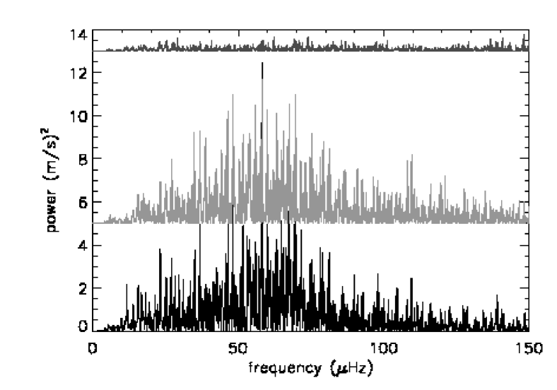
Figure 1: Power spectrum of $ϵ$ Ophiuchi. The lower black one is obtained by De Ridder et al. (2006b), the grey one in the middle is obtained from $\langle\mathrm{v}\rangle$ and the top one is obtained from the bisector velocity span. For clarity the latter two are shifted.

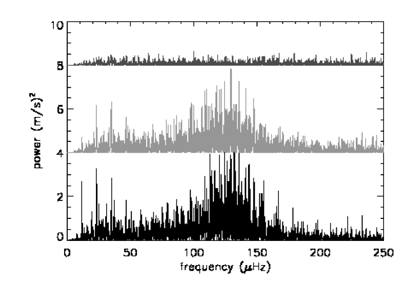
Figure 2: Power spectrum of $η$ Serpentis. The lower black one is obtained by Carrier et al. (2006), the grey one in the middle is obtained from $\langle\mathrm{v}\rangle$ and the top one is obtained from the bisector velocity span. For clarity the latter two are shifted.

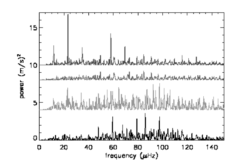
Figure 3: Power spectrum of $ξ$ Hydrae. The lower black one is obtained by Frandsen et al. (2002), the grey one is obtained from $\langle\mathrm{v}\rangle$. The two top power spectra are obtained from the bisector velocity span. The top one is the original, while the lower one is corrected for the 1 c d^-1 ($11.57\mu$Hz) frequency due to the diurnal cycle. For clarity the latter three power spectra are shifted.

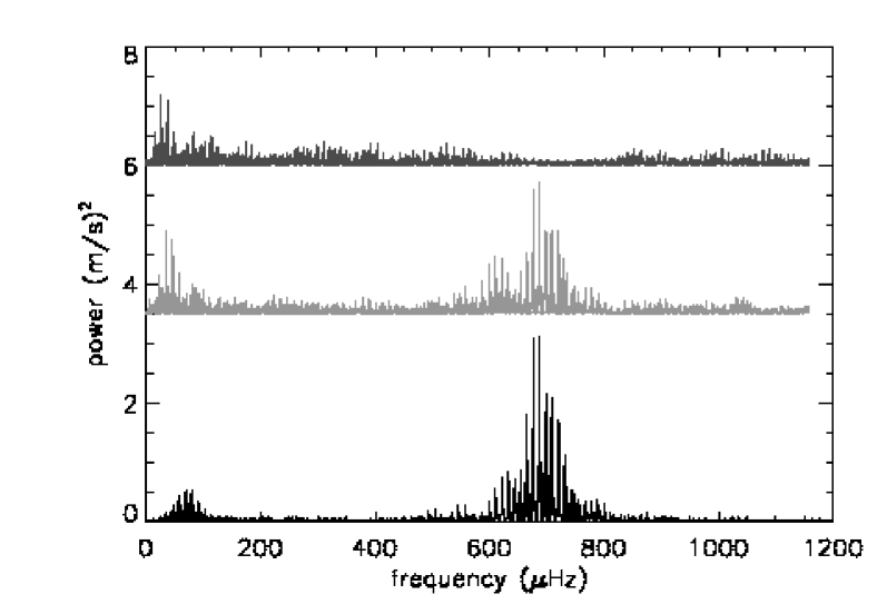
Figure 4: Power spectrum of $δ$ Eridani. The lower black one is obtained by Carrier et al. (2003), the grey one in the middle is obtained from $\langle\mathrm{v}\rangle$. The top power spectrum is obtained from the bisector velocity span. For clarity the latter two power spectra are shifted.

2.2 Cross correlation profiles

The line profile variations of the four pulsating red (sub)giants are analysed with moments (Aerts et al. 1992) and with the line bisector (Gray 2005). The moments are often used to analyse stellar oscillations excited by a heat mechanism, while the line bisector is usually adopted to discover planet signatures. Both methods can be applied to one single spectral line, but also to a cross correlation profile, which has an increased signal to noise ratio:

$$SNR_{cross-cor}=\sqrt{M<(SNR)^{2}>}$$ (1)

with $M$ the number of spectral lines used for the cross correlation and $<(SNR)^{2}>$ the average of the squared signal to noise ratios of each spectral line used. The cross correlation profiles are constructed from a mask in such a way that the weak, strong and blended lines are excluded. They are a good representation of an average spectral line of the star whenever the lines are formed at not too different line formation regions in the atmosphere.

Mathias & Aerts (1996) and Chadid et al. (2001) already performed a line profile analysis on cross correlation profiles for a $\delta$ Scuti star using moments (Aerts et al. 1992). Compared to the analysis of a single spectral line this only introduces some additional terms in the moments for which can be corrected. Furthermore, the line bisector analysis is widely used on cross correlation profiles (see e.g. Queloz et al. (2001a), Setiawan et al. (2003), Martínez Fiorenzano et al. (2005), Dall et al. (2006)). Dall et al. (2006) showed that the cross correlation bisector contains the same information as single line bisectors.

The red (sub)giants analysed in the present work show low amplitude radial velocity variations, which result in very small line profile variations. The INTER-TACOS (INTERpreter for the Treatment, the Analysis and the COrrelation of Spectra) software package developed at Geneva Observatory (Baranne et al. 1996), was used to cross correlate the observed spectrum with a mask containing atmospheric lines of red (sub)giants with a resolution of 100 m s^-1. On top of that we interpolated to a resolution of 10 m s^-1 to reach the highest possible precision in the computation of the moments.

2.3 Frequency analysis

In order to see whether the line moments and line bisector are sensitive enough to determine the very small line profile variations present in pulsating red (sub)giants, a frequency analysis is performed and compared with the frequencies obtained previously. Frandsen et al. (2002), De Ridder et al. (2006b), Carrier et al. (2006) and Carrier et al. (2003) used radial velocity variations, obtained with the optimum weight method described by Bouchy et al. (2001), for their frequency analysis.

2.3.1 Moments

A line profile can be described by its moments (Aerts et al. 1992). The first moment $\langle\mathrm{v}\rangle$ represents the centroid velocity of the line profile, the second moment $\langle\mathrm{v}^{2}\rangle$ the width of the line profile and the third moment $\langle\mathrm{v}^{3}\rangle$ the skewness of the line profile. The quantity $\langle\mathrm{v}\rangle$ is thus a particular measure of the radial velocity and should therefore show similar frequency behaviour. We expect it to perform less well than the radial velocity measure derived from the optimum weight method (Bouchy et al. 2001) (see below), but $\langle\mathrm{v}\rangle$ is a mode identification diagnostic (Aerts et al. 1992), while other radial velocity measures are not. This is why we re-compute and re-analyse the radial velocity from $\langle\mathrm{v}\rangle$ here.

Frequencies are determined with the conventional method of iterative sinewave fitting (‘prewhitening’). A Scargle periodogram (Scargle 1982) is used with frequencies between 0 and 15 cycles per day (c d^-1) (173.6 $\mu$Hz) and with a frequency step of 0.0001 c d^-1 (0.001 $\mu$Hz) for the red giants. For the subgiant frequencies between 0 and 150 c d^-1 and a frequency step of 0.001 c d^-1 are used. The significance of the frequencies is calculated with respect to the average amplitude of the periodogram after prewhitening as described in Kuschnig et al. (1997). The errors in the frequency are obtained with the method described by Breger et al. (1999) and have typical values of $10^{-4}$ c d^-1 ($10^{-9}\mu$Hz) for the giants and $10^{-3}$ c d^-1 ($10^{-8}\mu$Hz) for the subgiant.

The frequencies of $\langle\mathrm{v}\rangle$ are compared to the frequencies obtained from radial velocities derived from the optimum weight method, mentioned in earlier publications. In Figs 1, 2, 3 and 4 the power spectra of $ϵ$ Ophiuchi, $η$ Serpentis, $ξ$ Hydrae and $δ$ Eridani are shown, respectively. The lower black power spectra are the ones obtained by De Ridder et al. (2006b), Carrier et al. (2006), Frandsen et al. (2002) and Carrier et al. (2003), while the grey ones in the middle are obtained from $\langle\mathrm{v}\rangle$ in the present work.

Although the same data is used, a comparison is made between power spectra of two different representations of the radial velocity variations, computed with different methods. The radial velocity derived from the optimum weight method is intrinsically more precise than the one from $\langle\mathrm{v}\rangle$ of the cross correlation. It not only uses the full spectrum instead of a box shaped mask, but also relies on weights of the individual spectra. These differences influence the noise and the amplitudes in the power spectra. On top of that the reference point of each night is determined by the observation with the highest signal to noise ratio in case of the optimum weight method and by the average of the night in case $\langle\mathrm{v}\rangle$ is used. As nightly reference points are effectively a high pass filter, different filters induce differences at low frequencies in the power spectra.

Despite these differences the comparison between the power spectra in the literature and obtained from $\langle\mathrm{v}\rangle$ is very good, especially for $ϵ$ Ophiuchi and $δ$ Eridani. For $η$ Serpentis, the dominant frequencies obtained by Carrier et al. (2006) are slightly different. This is mainly due to the additional ELODIE data, which contains a substantial number of observations and therefore alters the time sampling of the data. In case only the CORALIE data are taken into account, the dominant frequencies match very well. For $\xi$ Hydrae the dominant frequencies obtained by Frandsen et al. (2002) are more distinct than those obtained from $\langle\mathrm{v}\rangle$. This is due to the low amplitude of this star, which implies a larger relative difference between the different computations of the radial velocity than for the other two giants. Nevertheless, the overall shape of the power spectra obtained from the radial velocity and from $\langle\mathrm{v}\rangle$ is comparable. The fact that $\langle\mathrm{v}\rangle$ shows the same behaviour as the radial velocity obtained with the method described by Bouchy et al. (2001), indicates that this moment diagnostic is able to detect low amplitude oscillations of red (sub)giants.

The behaviour of $\langle\mathrm{v}^{2}\rangle$ obtained from a cross correlation is not exactly the same as for a single spectral line. Chadid et al. (2001) show that the constant of a sinusoidal fit through $\langle\mathrm{v}^{2}\rangle$ is different in case of a cross correlation compared to a single spectral line. Furthermore, a fit through $\langle\mathrm{v}^{3}\rangle$ obtained from a cross correlation contains a non zero constant, which is not the case for a single spectral line. This indicates that we should be very cautious in interpreting the constants of the moments. Chadid et al. (2001) attribute the different behaviour of $\langle\mathrm{v}^{2}\rangle$ and $\langle\mathrm{v}^{3}\rangle$ obtained from cross correlation to the influence of possible blending with very faint lines which alters the absolute values of $\langle\mathrm{v}^{2}\rangle$ and $\langle\mathrm{v}^{3}\rangle$, but not their variation.

For the observed red giants, $\langle\mathrm{v}^{2}\rangle$ shows variations in the average value per night, which is probably caused by changing instrumental conditions. Although a correction for this behaviour is applied by shifting the values of each night to the average value of all observations, $\langle\mathrm{v}^{2}\rangle$ does not behave as predicted from theory. Frequencies for $\langle\mathrm{v}^{2}\rangle$ are expected to be: $\nu_{i}$, $\nu_{i}+\nu_{j}$ or $\nu_{i}-\nu_{j}$, with $\nu_{i,j}$ the frequencies obtained in $\langle\mathrm{v}\rangle$ (Mathias et al. 1994), but are not found in the observations. For all four stars, the frequencies obtained for $\langle\mathrm{v}^{3}\rangle$ are the same as for $\langle\mathrm{v}\rangle$, which is as expected.

2.3.2 Line Bisector

The line bisector is a measure of the displacement of the centre of the red and blue wing from the core of the spectral line at each residual flux. The line bisector is often characterised by the bisector velocity span, which is defined as the horizontal distance between the bisector positions at fractional flux levels in the top and bottom part of the spectral line, see for instance Brown et al. (1998). The bisector velocity span is supposed to remain constant over time in case of substellar companions.

The bisector velocity span is calculated in this work as the difference between the bisector at a fractional flux level of 0.80 and 0.20. The frequencies of the bisector velocity span are determined in the same way as the frequencies of the moments.

Bisector velocity spans are calculated for simulated spectral lines of stars pulsating with different modes, using $ϵ$ Ophiuchi’s amplitude. In case of noiseless line profiles and infinite mode lifetimes, the dominant frequency of modes with $m=0$ is $2\nu$, with $\nu$ the dominant frequency obtained for $\langle\mathrm{v}\rangle$. In case $m\neq 0$, $\nu$ is obtained as the dominant frequency. For infinite mode lifetimes the dominant frequency obtained for modes with $m=0$ is low, but at $2\nu$ the power spectrum also shows a clear excess. For modes with $m\neq 0$ we obtained $\nu$ as the dominant frequency. This is completely in line with the behaviour expected for $\langle\mathrm{v}^{2}\rangle$ (Aerts et al. 1992).

To give an estimate of the minimum signal to noise ratio needed to detect a dominant frequency, with the amplitude detected for $ϵ$ Ophiuchi in the bisector velocity span, we added white noise to the simulated spectral lines. These simulations reveal that for pulsations with infinite as well as finite mode lifetimes with $m=0$, a signal to noise ratio of 100 000 is not enough to reveal a frequency in the bisector velocity span, while a signal to noise ratio of order a few 10 000 would suffice for modes with $m\neq 0$. The signal to noise ratio of the cross correlation profiles of our targets does not exceed a few 1 000 (see Equation 1). This signal to noise level is much less than the minimum value needed to detect the oscillations.

The top graphs in Figs 1, 2, 3 and 4 show the power spectra of the bisector velocity span for $ϵ$ Ophiuchi, $η$ Serpentis, $ξ$ Hydrae and $δ$ Eridani, respectively. The bisector velocity spans for $ϵ$ Ophiuchi and $η$ Serpentis do not show any dominant frequency. The power spectrum of the bisector velocity span of $ξ$ Hydrae shows peaks at 1 c d^-1 ($11.57\mu$Hz) and at its 1 day aliases (Fig. 3 top). The aliases are due to the diurnal cycle and in case these are removed no dominant frequencies in the bisector velocity span can be seen (Fig. 3 second power spectrum from the top). For $δ$ Eridani the bisector velocity span shows some peaks at low frequencies, but from asteroseismological considerations solar like pulsations can not occur at these low frequencies in subgiants. These peaks are probably caused by instrumental effects. From the present test case, one can thus conclude that, at least for low amplitude oscillations, discrimination between exoplanet companions and pulsations is not possible with the bisector velocity span on data with realistic signal to noise ratio. This result is consistent with Dall et al. (2006).

3 Theoretical mode diagnostics

In order to characterise wavenumbers $(\ell,m)$ for the modes present in the red (sub)giants, the mathematical description of the line bisector (Brown et al. 1998) and of the moments (Aerts et al. 1992) are investigated.

Brown et al. (1998) introduced a mathematical description for the line bisector in terms of orthogonal Hermite functions. The Hermite coefficients $h_{i}$ describe the line shapes. Information on the oscillation mode, inclination and velocity parameters of the star was obtained by Brown et al. (1998) from a comparison with theoretically generated line profile variations during a pulsation cycle, assuming infinite mode lifetimes. To obtain the wavenumbers of the oscillations, the Hermite coefficients or bisector velocity span obtained from observations are compared with the ones calculated for the simulated line profiles. The main drawback of this description in Hermite functions is the lack of a pulsation theory directly coupled to the Hermite coefficients or bisector velocity span. For this reason we do not use it here.

The variations in the observed moments of the line profiles are compared with their theoretical expectations derived from oscillation theory (Aerts et al. 1992). The moments are a function of wavenumbers $\ell,m$, inclination $i$, pulsation velocity amplitude $\upsilon_{p}$, projected rotational velocity $\upsilon\sin i$ and intrinsic width of the line profile $\sigma$. The comparison is performed objectively with a discriminant (Aerts et al. (1992), Aerts (1996), Briquet & Aerts (2003)) which selects the most likely set of parameters ($\ell,m,i,\upsilon_{p},\upsilon\sin i,\sigma$). Due to the fact that several combinations of the wavenumbers and velocity parameters result in almost the same line profile variation, the “few” best solutions resulting from the discriminant should be investigated carefully before drawing conclusions about the mode identity.

The fact that $\langle\mathrm{v}\rangle$ and $\langle\mathrm{v}^{3}\rangle$ are sensitive to the very small line profile variations and the direct connection between the moments and pulsation theory makes moments, in principle, suitable for the analysis of pulsating red (sub)giants, provided that we test its robustness against small amplitudes and the finite lifetimes of the modes. This is what we have done in the present work.

3.1 Discriminant

In the present analysis the discriminant is determined for $\ell=0,1,2$, inclination angles ranging from $5\degr$ until $85\degr$ with steps of $1\degr$, projected rotational velocity $\upsilon\sin i$ and intrinsic width of the line profile $\sigma$ between 0 and 5 km s^-1 with steps of 0.5 km s^-1. Furthermore a limbdarkening coefficient $u(\lambda)$ of 0.5 is used (van Hamme 1993).

Due to the fact that the red (sub)giants show low amplitude variations, the discriminant might give inclination angles close to an inclination angle of complete cancellation (IACC) (Chadid et al. 2001). Complete cancellation occurs when the star is looked upon in such way that the contribution to $\langle\mathrm{v}\rangle$ of each point on the stellar disk exactly cancels out the contribution of another point on the stellar disk. Therefore the angles close to $0\degr$ and $90\degr$ are not taken into account, as well as solutions close to the IACC at $i=54.7\degr$ for $\ell=2,m=0$.

As the discriminant is designed for oscillations inducing moment variations larger than the equivalent width of the line (moment of order zero), a check needs to be performed whether this technique is applicable in the present work. Therefore three series of spectral line profiles with infinite lifetimes and different pulsation velocity amplitudes are generated using the 628 observation times of $ϵ$ Ophiuchi. The dominant frequency of $ϵ$ Ophiuchi, 5.03 c d^-1 (58.2 $\mu$Hz), is used as an input parameter at an inclination of $i=35\degr$ for wavenumbers $\ell=0,1,2$ with positive $m$ values, a projected rotational velocity $\upsilon\sin i=3.5$ km s^-1 and an intrinsic width $\sigma=4$ km s^-1. Furthermore, the equivalent width of the spectral lines is taken to be 10 km s^-1, while the minimum amplitude of the pulsation velocity ($\upsilon_{p}$) is 0.04 km s^-1 and increases with a factor of 10 for the different series. For these series the moments are calculated as well as the discriminant. For a pulsation velocity amplitude of 0.04 km s^-1, which resembles the data best, $\langle\mathrm{v}^{2}\rangle$ of modes with $m=0$ all show the expected harmonic of the frequency (Mathias et al. 1994), but with a different constant. The discriminant values only differ by an order of 0.01 km s^-1. This is also the case for a pulsation velocity amplitude of 0.4 km s^-1, which indicates that the discriminant is not suitable for the analysis of small line profile variations with an amplitude below 1 km s^-1. For a pulsation velocity amplitude of 4.0 km s^-1 the difference between the discriminant values increases and the correct mode is present among the best options. This indicates that the discriminant is a useful analysis tool for spectral line variations with amplitude larger than about half the equivalent width of the spectral line, but not for red (sub)giants.

3.2 Amplitude and phase distribution

Figure 5: The amplitude (left) and phase (right) distributions for simulated line profiles with infinite damping time at an inclination angle of $i=35\degr$. Top left: $\ell=0$, $m=0$, top right: $\ell=1$, $m=0$, middle left: $\ell=1$, $m=1$, middle right: $\ell=2$, $m=0$, bottom left: $\ell=2$, $m=1$, bottom right: $\ell=2$, $m=2$

As the discriminant is not useful in the present analysis, the spectral lines are investigated by comparing the amplitude and phase across the line profile with the ones obtained from simulations. This is the same procedure as used by Telting et al. (1997) for $β$ Cephei and by De Cat et al. (2005) for the complex line profile behaviour due to the multi periodic gravity mode oscillations in slowly pulsating B stars. The amplitude and phase for each velocity in the cross correlation profile are determined by fitting a harmonic function, with the dominant frequencies of $\langle\mathrm{v}\rangle$, to the flux values at each velocity pixel of the time series of spectra (Schrijvers et al. 1997). The amplitudes and phases as function of velocity determined from simulated line profiles with $\ell=0,1,2$, and positive $m$ values are shown in Fig. 5, assuming infinite lifetimes. The simulations are shown for $i=35\degr$, but the shape of the amplitude and phase distribution does not change significantly with inclination angle.

The amplitude and phase distribution across the line profile of $ϵ$ Ophiuchi, $η$ Serpentis, $ξ$ Hydrae and $δ$ Eridani are shown in Figs 6, 7, 8 and 9 respectively. The dominant frequencies obtained from $\langle\mathrm{v}\rangle$ are used for the harmonic fits at each velocity in the line profile. The frequencies obtained for each star are listed in Tables 2, 3, 4 and 5. The windowfunction for $η$ Serpentis changes slightly in case only CORALIE data is used compared to the one obtained from both CORALIE and ELODIE data (Carrier et al. 2006). For the CORALIE data we find an extra aliasfrequency of 0.17 c d^-1. The frequency 11.17 c d^-1, only obtained for the CORALIE data, is therefore an alias of the 10.33 c d^-1 frequency obtained by Carrier et al. (2006). The frequency $\nu=3.00$ c d^-1 for $δ$ Eridani is indicated in bold because this is an alias of the diurnal cycle of the observations and not due to solar like oscillations.

Table 2: Comparison between frequencies found in $\langle\mathrm{v}\rangle$ ($\nu_{\langle\mathrm{v}\rangle}$) and the ones found by De Ridder et al. (2006b) in the radial velocity of $ϵ$ Ophiuchi. The significance of $\nu_{\langle\mathrm{v}\rangle}$ is calculated with respect to the average amplitude of the periodogram after prewhitening as described by Kuschnig et al. (1997): $4\sigma\propto 99.9\%$ confidence interval, $3.6\sigma\propto 99\%$ confidence interval and $3.25\sigma\propto 95\%$ confidence interval.

$\nu_{\langle\mathrm{v}\rangle}$	$\nu_{\langle\mathrm{v}\rangle}$	significance	$\nu$	$\nu^{a}$
c d-1	$\mu$Hz		c d-1	$\mu$Hz
5.03	58.2	4.69$\sigma$	5.03	58.2
5.46	63.2	3.99$\sigma$	5.44	63.0
5.83	67.5	3.98$\sigma$	5.82	67.4
			4.59	53.1
3.17	36.7	3.43$\sigma$	4.17	48.3
			4.46	51.6
			5.59	64.7
			6.19	71.7
			5.18	59.9
			6.00	69.5
			6.43	74.4

Figure 6: The amplitude (top) and phase (bottom) distributions as a function of velocity across the line profile of $ϵ$ Ophiuchi for the three significant frequencies obtained from $\langle\mathrm{v}\rangle$: $\nu_{\langle\mathrm{v}\rangle}=5.03$  c d^-1 ($58.2\mu$Hz) (left) $\nu_{\langle\mathrm{v}\rangle}=5.46$  c d^-1 ($63.2\mu$Hz) (middle) and $\nu_{\langle\mathrm{v}\rangle}=5.83$  c d^-1 ($67.5\mu$Hz) (right). The mean radial velocity of the star, is found to be approximately $-9.4$ km s^-1.

Table 3: Comparison between frequencies found in $\langle\mathrm{v}\rangle$ and the ones found by Carrier et al. (2006) in the radial velocity of $η$ Serpentis. The significance (sign) of $\nu_{\langle\mathrm{v}\rangle}$ is calculated with respect to the average amplitude of the periodogram after prewhitening as described by Kuschnig et al. (1997): $4\sigma\propto 99.9\%$ confidence interval, $3.6\sigma\propto 99\%$ confidence interval and $3.25\sigma\propto 95\%$ confidence interval.

$\nu_{\langle\mathrm{v}\rangle}$	$\nu_{\langle\mathrm{v}\rangle}$	signi-	$\nu$	$\nu^{a}$	$\nu$	$\nu^{b}$
c d-1	$\mu$Hz	ficance	c d-1	$\mu$Hz	c d-1	$\mu$Hz
11.71	135.5	3.80$\sigma$	10.74	124.3	11.74	135.9
10.38	120.2	3.61$\sigma$	10.38	120.2	10.40	120.4
					11.49	133.0
					13.27	153.6
					10.96	126.8
					10.90	126.2
11.17	129.3	4.23$\sigma$	11.17	129.3	10.33	119.6
					11.69	135.3
					7.48	86.6
					7.28	84.3
					6.20	71.8

Figure 7: The amplitude (top) and phase (bottom) distributions as a function of velocity across the line profile of $η$ Serpentis for the significant frequencies obtained from $\langle\mathrm{v}\rangle$: $\nu_{\langle\mathrm{v}\rangle}=11.17$ c d^-1 ($129.3\mu$Hz) (left), $\nu_{\langle\mathrm{v}\rangle}=11.71$ c d^-1 ($135.5\mu$Hz) (middle) and $\nu_{\langle\mathrm{v}\rangle}=10.38$ c d^-1 ($120.2\mu$Hz) (right). The mean radial velocity of the star, is found to be approximately $9.4$ km s^-1.

Figure 8: The amplitude (top) and phase (bottom) distributions as a function of velocity across the line profile of $ξ$ Hydrae for the most dominant frequency obtained from $\langle\mathrm{v}\rangle$: $\nu_{\langle\mathrm{v}\rangle}=8.42$ c d^-1 ($97.5\mu$Hz). The mean radial velocity of the star, is found to be approximately $-4.6$ km s^-1.

Table 4: Comparison between frequencies found in $\langle\mathrm{v}\rangle$ and the ones found by Frandsen et al. (2002) in the radial velocity of $ξ$ Hydrae. The significance of $\nu_{\langle\mathrm{v}\rangle}$ is calculated with respect to the average amplitude of the periodogram after prewhitening as described by Kuschnig et al. (1997). A significance of $3\sigma\propto 85\%$ confidence interval.

$\nu_{\langle\mathrm{v}\rangle}$	$\nu_{\langle\mathrm{v}\rangle}$	significance	$\nu$	$\nu^{a}$
c d-1	$\mu$Hz		c d-1	$\mu$Hz
			5.1344(26)	59.43
			6.8366(27)	79.13
8.42	97.5	3.00$\sigma$	7.4265(29)	85.96
			8.2318(32)	95.28
			9.3507(33)	108.22
			8.7399(36)	101.16
			10.0287(43)	116.07
			9.0831(44)	105.13
			8.5339(40)	98.77

Table 5: Comparison between frequencies found in $\langle\mathrm{v}\rangle$ and the ones found by Carrier et al. (2003) in the radial velocity of $δ$ Eridani. The significance (sign) of $\nu_{\langle\mathrm{v}\rangle}$ is calculated with respect to the average amplitude of the periodogram after prewhitening as described by Kuschnig et al. (1997): $4\sigma\propto 99.9\%$ confidence interval, $3.6\sigma\propto 99\%$ confidence interval and $3.25\sigma\propto 95\%$ confidence interval.

$\nu_{\langle\mathrm{v}\rangle}$	$\nu_{\langle\mathrm{v}\rangle}$	significance	$\nu$	$\nu^{a}$
c d-1	$\mu$Hz		c d-1	$\mu$Hz
			43.55	504.0
			47.12	545.4
			49.59	573.9
			52.73	610.3
52.68	609.7	4.84$\sigma$	54.67	632.7
			56.54	654.4
			58.06	672.0
59.40	687.5	7.45$\sigma$	58.40	675.9
			60.65	702.0
61.08	706.9	6.01$\sigma$	62.08	718.5
60.25	697.3	4.08$\sigma$	62.27	720.7
57.55	666.1	4.45$\sigma$	64.55	747.1
65.28	755.6	3.71$\sigma$	66.28	767.1
			68.07	787.9
			75.63	875.4
3.00	34.7	5.89$\sigma$

Figure 9: The amplitude (top) and phase (bottom) distributions as a function of velocity across the line profile of $δ$ Eridani for the significant frequencies obtained from $\langle\mathrm{v}\rangle$: $\nu_{\langle\mathrm{v}\rangle}=59.40$ c d^-1 ($687.5\mu$Hz) (left), $\nu_{\langle\mathrm{v}\rangle}=61.08$ c d^-1 ($706.9\mu$Hz) (middle) and $\nu_{\langle\mathrm{v}\rangle}=52.68$ c d^-1 ($609.7\mu$Hz) (right). The mean radial velocity of the star, is found to be approximately $-6.3$ km s^-1.

4 Simulations

In order to test the robustness of moment diagnostics and the amplitude and phase behaviour across the line profiles against finite lifetimes of oscillation modes, spectral lines are generated with damped and re-excited modes. The moments of these lines are obtained and their dominant frequencies derived. Furthermore, the amplitude and phase distribution across the spectral line is investigated.

The simulations are done for a single lineforming region. Therefore, the simulated phase distributions are not necessarily comparable to the observed ones, which are averaged phase distributions over a whole range of line forming regions because they are based on a cross correlation function. Our interpretation will therefore mainly be based on the amplitude distribution which represents an average amplitude across the whole lineforming region considered in the cross correlation function.

4.1 Damping and re-excitation equations

A damped and re-excited oscillation mode is damped by a factor $e^{-\eta t}$, with $\eta$ the damping rate, and re-excited before it is able to damp out. As a consequence both the amplitude and the phase of the oscillation are time dependent:

$$f(t)=A(t)\sin(2\pi\nu t+\psi(t)).$$ (2)

To simulate such an oscillator we follow the description of De Ridder et al. (2006a), and we compute

$$f(t)=B(t)\sin(2\pi\nu t)+C(t)\cos(2\pi\nu t),$$ (3)

where we let the amplitudes $B$ and $C$ vary with a first order autoregressive process in a discrete time domain with time step $\Delta t$:

$$B_{n}=e^{-\eta\Delta t}B_{n-1}+\varepsilon_{n+1}$$ (4)

where $\varepsilon_{n+1}$ is a Gaussian distributed excitation kick. For more details we refer to De Ridder et al. (2006a). The above is applied to the equations for the pulsation velocity which are obtained by taking the time derivative of the displacement components mentioned in Section 3.2, Eq.(2) of De Ridder et al. (2002). Whenever rotation is neglected, the three spherical components of the pulsation velocity, i.e. $\upsilon_{r}$, $\upsilon_{\theta}$ and $\upsilon_{\varphi}$, for the damped and re-exited case become:

$$\upsilon_{r} = -\upsilon_{p}N_{\ell}^{m}P_{\ell}^{m}(\cos\theta)*$$ (5)

$$e^{-\eta(t-n\Delta t_{kick})}(B_{n}\sin(m\varphi+2\pi\nu t)+C_{n}\cos(m\varphi+2\pi\nu t)),$$

$$\upsilon_{\theta} = -K\upsilon_{p}N_{\ell}^{m}\frac{\partial}{\partial\theta}(P_{\ell}^{m}(\cos\theta))*$$ (6)

$$e^{-\eta(t-n\Delta t_{kick})}(B_{n}\sin(m\varphi+2\pi\nu t)+C_{n}\cos(m\varphi+2\pi\nu t)),$$

$$\upsilon_{\varphi} = -mK\upsilon_{p}N_{\ell}^{m}\frac{1}{\sin\theta}P_{\ell}^{m}(\cos\theta)*$$ (7)

$$e^{-\eta(t-n\Delta t_{kick})}(B_{n}\cos(m\varphi+2\pi\nu t)-C_{n}\sin(m\varphi+2\pi\nu t)),$$

with $\upsilon_{p}$ proportional to the pulsation amplitude, $N_{\ell}^{m}$ the normalisation factor for the spherical harmonics $Y_{\ell}^{m}(\theta,\varphi)\equiv P_{\ell}^{m}(\cos\theta)e^{im\varphi}$ and $K$ the ratio of the horizontal to the vertical velocity amplitude.

Line profiles with the same parameters as described in section 3.1 are generated with a damping time ($\eta^{-1}$) of two days (the estimate for $ξ$ Hydrae by Stello et al. (2004)). The used pulsation amplitude is 0.04 km s^-1. The moments, with the dominant frequencies and the amplitude and phase distribution across the line profiles are investigated.

4.2 Frequencies

$\langle\mathrm{v}\rangle$, $\langle\mathrm{v}^{2}\rangle$ and $\langle\mathrm{v}^{3}\rangle$ are determined for the generated series of line profiles and the frequencies are obtained in the same way as described in section 2.3.1. Rather than fitting a Lorenz profile to the power spectrum, we simply used the highest peak to obtain the oscillation frequency. This implies that the obtained frequencies differ slightly from the input frequency as predicted by the Lorenzian probability distribution. The frequencies obtained from $\langle\mathrm{v}^{3}\rangle$ are the same as the ones obtained for $\langle\mathrm{v}\rangle$, which is as expected from theory and also seen in the observations of the four red (sub)giants. None of the modes reveal a relation between the frequencies obtained from $\langle\mathrm{v}\rangle$ and $\langle\mathrm{v}^{2}\rangle$, which is due to the small amplitudes as described in section 2.3.1.

4.3 Amplitude and phase distribution

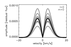
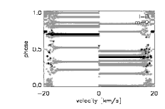
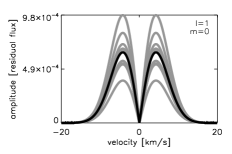
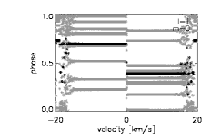
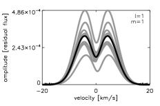
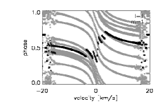
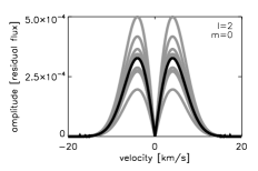
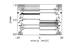
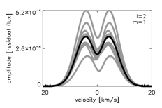
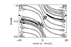
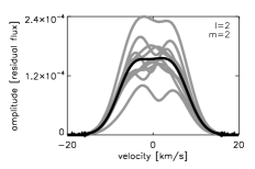
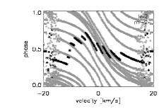
Figure 10: The amplitude (left) and phase (right) distributions for simulated line profiles with a two day damping time at an inclination angle of $i=35\degr$. For each mode ten different realisations are shown in grey, with the average shown in black. Top left: $\ell=0$, $m=0$, top right: $\ell=1$, $m=0$, middle left: $\ell=1$, $m=1$, middle right: $\ell=2$, $m=0$, bottom left: $\ell=2$, $m=1$, bottom right: $\ell=2$, $m=2$

The amplitude and phase distribution as a function of the velocity across the line profiles are investigated for the simulated spectral lines. The profiles for the cases with $\ell=0,1,2$ and positive $m$ values, with a damping time of $\eta=2$ days, are shown in Fig. 10. The dominant frequency obtained from $\langle\mathrm{v}\rangle$ is used for the harmonic fits. This frequency is different for each realisation due to the stochastic nature of the forcing. For each mode ten realisations are shown in grey, with the average shown in black. The shape of the amplitude of axisymmetric and tesseral modes do not change, although the amplitudes per velocity pixel can have different values for different realisations. The drop to zero amplitude in the centre of the line is very characteristic for all the amplitude distributions. However, for the sectoral modes, the shape and value of the amplitudes may be different for different realisations and the amplitude distribution does not necessarily drop in the centre of the line for such modes. The behaviour does not change significantly with inclination.

5 Interpretation

The amplitude distribution across the line profile is used for mode identification, as in Telting et al. (1997) and De Cat et al. (2005). For each star we find different distributions for different dominant mode frequencies. This clearly indicates that modes with different wavenumbers $(\ell,m)$ must be present in the data. Thus, we detect non-radial modes in the observed cross correlation profiles. In order to identify the wavenumbers of the individual modes, observed amplitude distributions are compared with simulated ones, as is commonly done for mode identification. Only very recently, Zima (2006) implemented a statistical measure to quantify the identification of $(\ell,m)$ as a function of amplitude across the profile for modes with infinite lifetime. A similar quantitative measure in the case of damped oscillations is not yet available, but visual inspection of amplitude diagrams allows a clear discrimination between axisymmetric and non-axisymmetric modes which is what we do here, based on simulations. The averaged amplitudes over different realisations (indicated in black in Fig. 10) are used for this comparison, keeping in mind that the observations are single realisations. Due to the fact that single realisations of different modes are in some cases comparable, different sets of wavenumbers are occasionally likely for observed modes.

For $ϵ$ Ophiuchi the amplitude of the first frequency $\nu=5.03$ c d^-1 ($58.2\mu$Hz) resembles the one of modes with $\ell=2$, $m=2$ mode. The mode with frequency $\nu=5.46$ c d^-1 ($63.2\mu$Hz) resembles an $m=1$ mode, although it does not exclude an $m=0$ mode. The mode with $\nu=5.83$ c d^-1 ($67.5\mu$Hz) resembles an $\ell=2$, $m=2$ mode.

The modes with frequency $\nu=11.17$ c d^-1 ($129.3\mu$Hz) and $\nu=11.71$ c d^-1 ($135.5\mu$Hz) obtained for $η$ Serpentis resembles a realisation of the $\ell=2$, $m=2$ mode, while the mode with the third frequency ($\nu=10.38$ c d^-1 ($102.2\mu$Hz)) is likely to have $m=0$.

For $ξ$ Hydrae the most dominant frequency $\nu=8.42$ c d^-1 ($97.5\mu$Hz) reveals a mode with either $m=0$ or $m=1$.

For $δ$ Eridani the dominant mode ($\nu=59.40$ c d^-1 ($687.5\mu$Hz)) resembles an $m=1$, while the second one ($\nu=61.08$ c d^-1 ($706.9\mu$Hz)) is characteristic for an $m=0$ mode. The third mode ($\nu=52.68$ c d^-1 ($609.7\mu$Hz)) shows an additional dip in the second peak, but $m=1$ as well as $m=0$ seem to be possible.

From the comparison of the observations with the simulations we can conclude that we see modes with $m\neq 0$ and thus non-radial modes among the dominant modes in the (sub) giants. This result is robust against a change in the value of the inclination angle for the simulations.

6 Discussion and conclusions

We have implemented a line profile generation code for damped and re-excited solar like oscillations. We found that the quantities $\langle\mathrm{v}\rangle$, $\langle\mathrm{v}^{3}\rangle$ and amplitude across the profile are good line diagnostics to characterise these oscillations. Our simulations were made for a single lineforming region while we compared them with cross correlation profiles based on a mask. For this reason, the phase variations across the profile are difficult to interpret, since they are an average over the depth in the atmosphere, and this average depends on the shape of the eigenfunctions. Moreover, we learned from our simulations that the phase behaviour can be quite different for realisations, as illustrated in Fig. 10. More extensive simulations across the depth would be needed to interpret the observed phase behaviour in detail. In order to do so, we would need to know the shape of the excited eigenmodes as a function of depth in the outer regions of the star.

From the frequency analysis performed on the bisector velocity span, it becomes clear that it is not a good diagnostic to unravel solar like oscillations.

Individual mode identification is not yet possible with the method used in the present work. This is not surprising because we did a first exploration of how well-working methods for modes with infinite lifetimes could be adapted for damped oscillations. The discriminant of the moments is not useful at the low amplitudes present in the sub(giants) investigated in the present work. Nevertheless, from the resemblance between the observed amplitude distribution with the simulated ones, and comparison between different modes of the same star, we presented clear observational evidence for modes with different m-values in the same star for three of our four examples, i.e. non-radial modes are present in red (sub)giants. The amplitudes for $ξ$ Hydrae are too low to make firm conclusions, and since we see only one frequency in the line profile variations, a comparison of the amplitude shapes for different modes is not possible. Therefore we can not exclude that this star has only radial modes as proposed by Frandsen et al. (2002).

Dziembowski et al. (2001) and Houdek & Gough (2002) show theoretically that stochastically excited radial pulsation modes are most likely to be observed in red giants. They predict that, for non-radial modes, damping effects will have influence in the p-mode cavity as well as in the g-mode cavity, while for radial modes only damping in the p-mode cavity is present. Therefore, according to this theory, radial modes are less severely influenced by damping than non-radial modes. Our result pointing towards the presence of non-radial modes, calls for a re-evaluation of the theoretical predictions.