A statistically-selected Chandra sample of 20 galaxy clusters – I. Temperature and cooling time profiles

Abstract

We present an analysis of 20 galaxy clusters observed with the Chandra X-ray satellite, focussing on the temperature structure of the intracluster medium and the cooling time of the gas. Our sample is drawn from a flux-limited catalogue but excludes the Fornax, Coma and Centaurus clusters, owing to their large angular size compared to the Chandra field-of-view. We describe a quantitative measure of the impact of central cooling, and find that the sample comprises 9 clusters possessing cool cores and 11 without. The properties of these two types differ markedly, but there is a high degree of uniformity amongst the cool core clusters, which obey a nearly universal radial scaling in temperature of the form $T\propto r^{\sim 0.4}$, within the core. This uniformity persists in the gas cooling time, which varies more strongly with radius in cool core clusters ($t_{\mathrm{cool}}\propto r^{\sim 1.3}$), reaching $t_{\mathrm{cool}}<1\,$Gyr in all cases, although surprisingly low central cooling times ($<5\,$Gyr) are found in many of the non-cool core systems. The scatter between the cooling time profiles of all the clusters is found to be remarkably small, implying a universal form for the cooling time of gas at a given physical radius in virialized systems, in agreement with recent previous work. Our results favour cluster merging as the primary factor in preventing the formation of cool cores.

1 Introduction

Clusters of galaxies are uniquely suitable environments for studying galaxy formation and evolution, as well as excellent cosmological tools for measuring the fundamental parameters of the Universe. A study of the scaling properties of clusters, which span roughly two decades in mass, is one of the best means of tackling both these objectives, and many analyses have been conducted on this basis, establishing broad trends and quantifying departures from simple self-similarity (e.g. Edge & Stewart, 1991b; Markevitch et al., 1998; Helsdon & Ponman, 2000; Fukazawa et al., 2004).

Increasingly, however, attention is shifting towards a more complete understanding of cluster physics, focussing in particular on the scatter in these scaling relations. With current generation telescopes, we are reaching the point where the precision of scaling relations is limited by systematic effects rather than measurement errors. Further progress requires a better knowledge of cluster physics to understand the sources of intrinsic scatter in these relations. Not only does this hold great potential for understanding galaxy evolution, it also promises to hone cluster observables as proxies for mass, which will be vital in extracting precise cosmological constraints from forthcoming large cluster surveys.

Since the cooling time of gas in the centres of most clusters is short compared to their age, radiative cooling would be expected to play an important role in cluster physics. However, many clusters do not show strong signs of cooling, possibly as a result of disruption caused by merging and associated shock heating of the gas, or else non-gravitational energy input (e.g. from AGN), or even heat redistribution via conduction or mixing. Moreover, even where cooling dominates, its progress is apparently impeded (see the recent review by Peterson & Fabian, 2006, and references therein), by processes which may well relate to these same phenomena. Whatever the explanation, it is clear that clusters can be separated into two distinct categories, according to the presence or absence of a ‘cool core’ (Peres et al., 1998; Bauer et al., 2005), where radiative heat losses have significantly lowered the central temperature of the gas. It is the combination of cool core and non cool core systems in the cluster population which accounts for much of the intrinsic scatter in scaling relations.

While cool core clusters have tended to be relatively well-studied, non-cool core clusters have received less attention in scaling relation analyses. Consequently there is great potential for exploring cluster physics by comparing the properties of the two types of clusters. This aim of this work is to investigate precisely this comparison, by focussing on a systematically selected sample of clusters, using data from the Chandra satellite, to allow a high-resolution study of the core properties of the intracluster medium (ICM).

Previous detailed studies of the temperature structure of the hot gas in clusters have generally concentrated on the most relaxed (i.e. morphologically regular) clusters (e.g. Sanderson et al., 2003; Piffaretti et al., 2005; Vikhlinin et al., 2005), which frequently possess cool cores. In this work, we have compiled a statistically selected sample of 20 clusters, to provide a more rigorous selection process. This naturally includes a larger number of non-cool core and perhaps less-relaxed clusters, which are more representative of the cluster population as a whole. We have subjected these 20 systems to a non-parametric analysis, so as to avoid any model-dependent biases in the comparison of cool core (CC) and non-CC systems. Furthermore, in restricting the analysis to X-ray data taken with the Chandra satellite, we are able to exploit the unrivalled spatial resolution of this telescope, to permit a detailed examination of the inner regions of the ICM, where the impact of radiative cooling is most pronounced.

Throughout this paper we adopt the following cosmological parameters; $H_{0}=70$$\mbox{~{}km}\mbox{~{}s}^{-1}\mbox{~{}Mpc}^{-1}\,$, $\Omega_{\mathrm{m}}=0.3$ and $\Omega_{\Lambda}=0.7$. Throughout our spectral analysis we have used xspec 11.3.1, incorporating the solar abundance table of Grevesse & Sauval (1998), which is different from the default abundance table. Typically this results in larger Fe abundances, by a factor of $\sim$1.4. All errors are 1$\sigma$, unless otherwise stated.

2 Sample Selection and Properties

The sample comprises the 20 highest flux clusters drawn from the 63 cluster, flux-limited sample of Ikebe et al. (2002), excluding those objects with extremely large angular sizes (the Coma, Fornax and Centaurus clusters), which are difficult to observe with Chandra owing to its limited field of view. Some basic properties of this sample are listed in Table 1. The Ikebe et al. flux-limited sample was constructed from the HIFLUGS sample of Reiprich & Böhringer (2002), additionally selecting clusters lying above an absolute galactic latitude of 20 degrees and located outside of the Magellanic Clouds and the Virgo Cluster regions.

Fig. 1 shows the cluster redshift as a function of mean X-ray temperature, excluding any cool core (see Section 4.1). The temperature errors are generally too small to be seen, and have been omitted for clarity. The point style differentiates between those clusters possessing a significant cool core and those without. The cool core classification scheme is described in Section 4.2.

Figure 1: Cluster mean temperature within 0.1–0.2 $r_{\mathrm{500}}$ as a function of redshift, labelled according to the presence of a cool core. Temperature errors have been omitted for clarity. Redshifts are taken from the NASA Extragalactic Database (NED).

Name	Obsida	Detectorb	RA	Dec.	Redshift	HI Columnc	Mean kTd	$r_{\mathrm{500}}$	Notese
			(J2000)	(J2000)		($\times 10^{20}$ cm-2)	(keV)	(kpc)
NGC 5044	798	S	198.850	-16.385	0.008	4.9	1.19 ${}^{+0.03}_{-0.02}$	436	–
Abell 262	2215	S (VF)	28.194	36.152	0.016	5.4	2.34 ${}^{+0.06}_{-0.06}$	668	–
Abell 4038	4188	I (VF)	356.928	-28.143	0.030	1.6	3.02 ${}^{+0.17}_{-0.17}$	784	F, T
Abell 1060	2220	I (VF)	159.181	-27.526	0.012	4.8	3.19 ${}^{+0.07}_{-0.07}$	812	F, T
Abell 1367	514	S	176.191	19.699	0.022	2.3	3.28 ${}^{+0.11}_{-0.10}$	826	T
2A0335+096	919	S	54.669	9.970	0.035	17.9	3.47 ${}^{+0.14}_{-0.12}$	856	–
Abell 2147	3211	I (VF)	240.567	15.963	0.035	3.4	4.17 ${}^{+0.14}_{-0.14}$	961	F, T
Abell 2199	497	S	247.160	39.551	0.030	0.9	4.36 ${}^{+0.13}_{-0.11}$	989	–
Abell 496	931	S	68.408	-13.262	0.033	4.6	5.91 ${}^{+0.58}_{-0.56}$	1200	–
Abell 2256	1386	I	256.041	78.648	0.058	4.1	6.08 ${}^{+0.30}_{-0.31}$	1220	T
Abell 1795	493	S (VF)	207.219	26.590	0.062	1.2	6.30 ${}^{+0.17}_{-0.17}$	1250	–
Abell 3558	1646	S (VF)	201.987	-31.496	0.048	3.9	6.64 ${}^{+0.34}_{-0.51}$	1290	T
Abell 85	904	I	10.460	-9.303	0.059	3.4	6.65 ${}^{+0.14}_{-0.14}$	1290	–
Abell 3571	4203	S (VF)	206.869	-32.864	0.039	3.7	6.71 ${}^{+0.15}_{-0.42}$	1300	F, T
Abell 3667	889	I	303.129	-56.841	0.056	4.7	7.39 ${}^{+0.27}_{-0.27}$	1380	T
Abell 478	1669	S	63.356	10.466	0.088	15.1	7.97 ${}^{+0.18}_{-0.18}$	1450	–
Abell 401	518	I	44.739	13.578	0.074	10.5	8.35 ${}^{+0.43}_{-0.61}$	1490	T
Abell 2029	4977	S	227.734	5.745	0.077	3.0	9.11 ${}^{+0.20}_{-0.20}$	1570	–
Abell 2142	1196	S	239.585	27.232	0.091	4.2	9.45 ${}^{+0.65}_{-0.65}$	1610	–
Abell 3266	899	I (VF)	67.815	-61.456	0.055	1.6	9.86 ${}^{+0.53}_{-0.54}$	1650	F, T

Table 1: Some basic properties of the sample, listed in order of increasing temperature. Coordinates are the centroids used in the X-ray analysis. ^aChandra observation identifier; ^bDenotes either ACIS-I or ACIS-S (observations telemetered in very faint mode are marked with VF); ^cGalactic HI column, interpolated to the cluster centroid using the data of Dickey & Lockman (1990); ^dThe mean temperature measured between 0.1–0.2 $r_{\mathrm{500}}$ (see Section 4.1); ^eAn “F” indicates that the galactic absorption was frozen at the HI value for the analysis, while “T” marks those clusters for which the projected $T(r)$ was used for the 3d $T(r)$. All errors are 68% confidence.

3 Data Reduction

The data analysis and reduction were performed with version 3.2.2 of the standard software — Chandra Interactive Analysis of Observations (ciao), incorporating caldb version 3.1. For all the observations a new level 2 events file was generated from the level 1 events file downloaded from the Chandra archive. This ensures that the latest calibration information is applied uniformly to the data, irrespective of when the observations were made.

The following procedure was followed for each observation dataset. According to which CCD chips were used in the observation, a different light curve was extracted for CCD chips 5 and 7 separately and the remaining, front-illuminated chips combined. The recommended criteria for energy extraction and time binning were used. Flares were identified and excluded with the sigma clipping algorithm implemented in the ciao task ‘lc_clean’, using the median light curve value to provide a robust initial estimate of the quiescent mean level.

Cosmic ray events were identified and excluded using the ciao task ‘acis_run_hotpix’, and those found in this manner were extracted separately and examined to check that photons from the cluster itself were not misidentified. A new level 1 events file was produced by reprocessing the resulting events file, to apply the latest gain file. Corrections were applied for the effects of charge transfer inefficiency (CTI) and time-dependent gain variation, where necessary. Bad columns and hot pixels were then excluded, and only events with Advanced Satellite for Cosmology and Astrophysics (ASCA) grades 0, 2, 3, 4, and 6 were retained. Subsequently, a new level 2 events file was generated by reprocessing this modified level 1 events data set. For those observations telemetered in very faint (VF) mode (indicated in column 3 of Table 1), the extra background event flagging and removal that this enables was performed in both the main and corresponding blank sky datasets.

Owing to the close proximity of the clusters in this sample, emission from the target fills the entire Chandra field of view in most cases. It was therefore necessary to employ separate background events files for each observation, using the Markevitch blank-sky data sets. To allow for small variations in the particle background level between the blank-sky fields and the target observation, we rescaled the effective exposure of the background data sets according to the ratio of count rates in the particle-dominated 7–12 keV energy band. This ratio was calculated for those CCD chips not considered part of the main detector (i.e. excluding chips 0-3 for ACIS-I and chip 7 for ACIS-S observations). Generally there is good agreement between the ratios found for different chips in a given observation. To avoid the bias caused by contaminating point sources in the determination of the background rescale factors, we identified and excluded such features using the iterative method described in Sanderson et al. (2005).

To gauge the sensitivity of our results to variations in the normalization of the blank sky datasets, we investigated its impact on our analysis of Abell 4038 (mean temperature $\sim$3 keV) — the cluster most susceptible to this effect (i.e. where the background is most dominant). We refitted spectra from our annular profile (see Section 4.3), separately adjusting the background normalization by 10 per cent higher and lower. In the outermost annulus, this biased the recovered temperature by roughly 1$\sigma$, in the direction of increasing temperature with higher background. However, the bias rapidly diminishes for the inner annuli, dropping below 0.3$\sigma$ for the 3rd innermost spectrum. It is clear, therefore, that our results are not sensitive to uncertainties associated with the use of blank sky background datasets.

4 Data Analysis

4.1 Cluster Mean Temperature and Fiducial Radius

The primary focus of this study is on cluster core properties, and we have therefore chosen to devote our analysis to the main CCD chips for each of the two detectors, i.e. chips 0–3 for ACIS-I and chip 7 for ACIS-S. For the spectral fitting, weighted response matrix files (RMFs) were generated using the ciao task ‘mkacisrmf’. However, for some observations this was not possible (as indicated in Section 5), owing to a lack of calibration data suitable for mkacisrmf, and so the older task ‘mkrmf’ was used instead. In each case the correct gain file was used, appropriate as described in the ciao documentation.

In a scaling study such as this, it is important to normalize observable quantities appropriately, to provide a fair comparison between clusters of different sizes. The key parameters of interest are mean gas temperature and characteristic radius, and we outline below a simple scheme in which both these quantities are determined self-consistently. Our fiducial radius corresponds to an overdensity of 500 with respect to the critical density of the Universe. This radius, $r_{\mathrm{500}}$, is commonly used for scaling studies and corresponds to roughly 2/3 of $r_{\mathrm{200}}$ (Sanderson & Ponman, 2003).

We defer a full mass profile analysis and direct determination of overdensity radii to a later paper, and adopt in this work a simple, empirically calibrated proxy for the total mass within $r_{\mathrm{500}}$, based on the mean temperature, derived from the $M-T_{\mathrm{X}}$ relation of Finoguenov et al. (2001). This has the advantage of permitting a direct comparison with other observations where poorer data quality prevents a full mass analysis being performed. For a cluster of redshift, $z$, the radius is given by (Willis et al., 2005)

$$r_{\mathrm{500}}=\frac{391\times\overline{T}^{0.63}}{E(z)}\,\,\mathrm{kpc}$$ (1)

where,

$$E(z)=(1+z)\sqrt{1+(z\,\,\Omega_{\mathrm{m}})+\frac{\Omega_{\mathrm{\Lambda}}}{(1+z)^{2}}-\Omega_{\mathrm{\Lambda}}}\,\,.$$ (2)

In calibrating the temperature-radius relation using observed clusters, we avoid the bias inherent in equivalent relations derived from numerical simulations, which tend to overestimate the virial radii of the coolest haloes (Sanderson et al., 2003). In using the above expression for $r_{\mathrm{500}}$ we have not allowed for the effects of evolution in the overdensity factor (i.e. the ‘500’) with redshift. However, for such a low redshift sample, the impact of this evolution is negligible.

The mean cluster temperature, $\overline{T}$, is measured from the spectrum extracted within 0.1–0.2 $r_{\mathrm{500}}$, thus excluding the central region where the effects of strong gas cooling can contaminate the X-ray emission. The combination of $\overline{T}$ and $r_{\mathrm{500}}$ are determined iteratively, by extracting an initial spectrum, finding the best-fit temperature, then using this to estimate $r_{\mathrm{500}}$, and repeating the process until convergence is achieved.

Name	Mean kT	Core kTa	kT Ratiob	$R_{500}$	CC significancec	Bautz-Morgan Type	Notesd
	(keV)	(keV)		(kpc)
NGC 5044	1.19 ${}^{+0.03}_{-0.02}$	$0.88^{+0.00}_{-0.00}$	$1.35^{+0.03}_{-0.03}$	$437^{+6}_{-6}$	11.7*	–	C, F
Abell 262	2.34 ${}^{+0.06}_{-0.06}$	$1.82^{+0.02}_{-0.02}$	$1.28^{+0.04}_{-0.04}$	$667^{+11}_{-11}$	7.9*	III	C
Abell 4038	3.02 ${}^{+0.17}_{-0.17}$	$3.26^{+0.14}_{-0.13}$	$0.93^{+0.07}_{-0.07}$	$785^{+28}_{-28}$	-1.1	III	–
Abell 1060	3.19 ${}^{+0.07}_{-0.07}$	$3.40^{+0.04}_{-0.05}$	$0.94^{+0.02}_{-0.02}$	$811^{+12}_{-12}$	-2.6	III	–
Abell 1367	3.28 ${}^{+0.11}_{-0.10}$	$3.32^{+0.10}_{-0.09}$	$0.99^{+0.04}_{-0.04}$	$826^{+17}_{-16}$	-0.3	II-III	M, R
2A0335+096	3.47 ${}^{+0.14}_{-0.12}$	$2.34^{+0.03}_{-0.03}$	$1.48^{+0.06}_{-0.06}$	$857^{+22}_{-18}$	8.2*	–	C, F, M
Abell 2147	4.17 ${}^{+0.14}_{-0.14}$	$4.82^{+0.37}_{-0.19}$	$0.87^{+0.06}_{-0.06}$	$961^{+20}_{-20}$	-2.3	III	M
Abell 2199	4.36 ${}^{+0.13}_{-0.11}$	$3.93^{+0.04}_{-0.04}$	$1.11^{+0.03}_{-0.03}$	$989^{+18}_{-15}$	3.4*	I	C
Abell 496	5.91 ${}^{+0.58}_{-0.56}$	$3.58^{+0.11}_{-0.11}$	$1.65^{+0.17}_{-0.17}$	$1197^{+75}_{-70}$	3.9*	I	F
Abell 2256	6.08 ${}^{+0.30}_{-0.31}$	$5.64^{+0.45}_{-0.50}$	$1.08^{+0.11}_{-0.11}$	$1220^{+38}_{-38}$	0.7	II-III	F, M, R
Abell 1795	6.30 ${}^{+0.17}_{-0.17}$	$4.88^{+0.06}_{-0.06}$	$1.29^{+0.04}_{-0.04}$	$1246^{+21}_{-21}$	7.5*	I	C, F
Abell 3558	6.64 ${}^{+0.34}_{-0.51}$	$6.04^{+0.32}_{-0.31}$	$1.10^{+0.09}_{-0.09}$	$1288^{+42}_{-62}$	1.1	I	–
Abell 85	6.65 ${}^{+0.14}_{-0.14}$	$4.80^{+0.06}_{-0.06}$	$1.38^{+0.03}_{-0.03}$	$1290^{+17}_{-17}$	11.4*	I	F, M, R
Abell 3571	6.71 ${}^{+0.15}_{-0.42}$	$7.85^{+0.17}_{-0.17}$	$0.85^{+0.04}_{-0.04}$	$1297^{+19}_{-51}$	-3.6	I	M
Abell 3667	7.39 ${}^{+0.27}_{-0.27}$	$6.76^{+0.18}_{-0.42}$	$1.09^{+0.06}_{-0.06}$	$1378^{+32}_{-32}$	1.5	I-II	F, M, R
Abell 478	7.97 ${}^{+0.18}_{-0.18}$	$6.00^{+0.07}_{-0.07}$	$1.33^{+0.03}_{-0.03}$	$1446^{+21}_{-21}$	9.6*	–	C,F
Abell 401	8.35 ${}^{+0.43}_{-0.61}$	$8.21^{+0.50}_{-0.63}$	$1.02^{+0.09}_{-0.09}$	$1488^{+48}_{-68}$	0.2	I	M
Abell 2029	9.11 ${}^{+0.20}_{-0.20}$	$7.18^{+0.07}_{-0.07}$	$1.27^{+0.03}_{-0.03}$	$1572^{+21}_{-21}$	8.9*	I	F
Abell 2142	9.45 ${}^{+0.65}_{-0.65}$	$7.81^{+0.33}_{-0.33}$	$1.21^{+0.10}_{-0.10}$	$1610^{+71}_{-69}$	2.1	II	F, M
Abell 3266	9.86 ${}^{+0.53}_{-0.54}$	$9.48^{+0.37}_{-0.37}$	$1.04^{+0.07}_{-0.07}$	$1653^{+57}_{-57}$	0.6	I-II	M

Table 2: Detailed properties of the sample, listed in order of increasing temperature. ^aThe core temperature measured within 0.1 $r_{\mathrm{500}}$; ^bRatio of mean to core temperature; ^cNumber of sigma difference from unity (Cool-core clusters are marked with “*”). ^dClusters with detectable cavities in the ICM are marked with “C”, cold front clusters are marked with “F”, probable merger clusters are marked with “M”, clusters with radio relics are marked with “R”. All errors are 68% confidence.

Figure 2: A comparison of the mean temperatures from this work and those of Ikebe et al. (2002), showing the line of equality.

Fig. 2 shows a comparison of the mean temperatures derived with those from the original ASCA analysis of Ikebe et al. (2002), who used a 2 temperature fit to correct for the effects of any cool core. There is good agreement below $\sim$5 keV, but above this our temperatures are systematically hotter in almost every case, for both CC and non-CC clusters. However, this behaviour is most likely the result of differences in the regions from which spectra were extracted in the two analyses. The most massive clusters have large angular sizes, which are significantly larger than the Chandra, but not ASCA, field-of-view. Since the temperature almost always declines beyond any cool core (e.g. Markevitch, 1998; Vikhlinin et al., 2005; Piffaretti et al., 2005), this would lead to a higher mean temperature measured with Chandra.

4.2 Cool Core Clusters

Having determined the cluster mean temperature, unbiased by the effects of central gas cooling, the spectrum of the core region ($<$0.1 $r_{\mathrm{500}}$) was extracted separately and fitted as before to yield a core temperature (see Table 2). A comparison between this core temperature and the mean (core-excluded) temperature can then be used to quantify the influence of central cooling. By considering the ratio of the mean to the core temperature as a discriminator, we define cool core (CC) clusters as those systems for which this ratio exceeds unity at greater than 3$\sigma$ significance. This provides a clean separation of the sample into 9 CC and 11 non-CC clusters, with a mean ratio and standard deviation of 1.35/0.15 and 1.0/0.11, respectively.

For comparison, in a recent Chandra study Bauer et al. (2005) find that at least 55 per cent of their sample of 38 X-ray luminous clusters show signs of mild cooling, with 34 per cent displaying evidence of strong cooling. According to the definition used by Bauer et al., all the clusters in our sample could be classified as having a cool core (cooling time, $t_{\mathrm{cool}}$$<$ 10 Gyr). However, their sample is more distant ($z\sim$ 0.15–0.4), and they are correspondingly less able to resolve the inner parts of the ICM where the gas cooling time is lowest and possibly falls below 10 Gyr in many cases. The older study of Peres et al. (1998) reported a cool-core fraction of 70 per cent, based on lower-resolution ROSAT observations of a complete sample of the 55 brightest clusters in the sky in the 2–10 keV band. However, their definition of a cool core is different again, requiring that the upper limit to the central $t_{\mathrm{cool}}$ be less than the assumed age for the cluster.

In any case, both Bauer et al. (2005) and Peres et al. (1998) base their definition of a cool-core on the gas cooling time which, as they demonstrate, is clearly capable of reaching low values ($\sim$few Gyr) in most — perhaps all — clusters (see also Section 6.2). By casting our definition in terms of a significant temperature decrease in the inner 0.1$r_{\mathrm{500}}$, we are able to identify clusters where radiative cooling has demonstrably impacted the gas properties in a substantial way, beyond merely forming at least some gas with a low cooling time.

4.3 Spectral Profiles and Deprojection Analysis

In order to study the spatial variation of gas temperature, a projected temperature profile was obtained for each cluster. Spectra were extracted in a series of concentric annuli, centred on the peak of the X-ray emission. The radial bins were chosen to enclose a fixed number of net cluster counts between 1000 and 3000, depending on the quality of the observation. Each spectrum was fitted with an absorbed APEC model, as above, to yield the best-fit temperature. A characteristic radius was assigned to each annulus using the emission-weighted approximation of McLaughlin (1999),

$$r=\left[0.5\left(r_{\mathrm{out}}^{3/2}+r_{\mathrm{in}}^{3/2}\right)\right]^{2/3}.$$ (3)

To derive estimates of the 3 dimensional gas temperature, we used the xspec PROJCT model to deproject the spectral profiles under the assumption of spherical geometry. The deprojection is quite slow and susceptible to strong noise fluctuations, so we used a smaller number of coarser annular bins — between 10 and 20, according to data quality. To stabilize the fitting, the absorbing column and gas metallicity we fixed at values obtained by fitting each annulus separately prior to the deprojection. For some clusters, it was necessary to freeze the absorbing column at the galactic HI value (as detailed in Table 1), since unfeasibly low values were otherwise obtained in many of the annular bins. However, we verified that in those bins where the absorbing column was able to be fitted, the optimum values were fully consistent with the HI inferred measurement. Moreover, we found no indication of any radial trend in absorbing column in these cases, which might point to problems with the calibration. Similarly, in a number of cases the deprojected temperature had to be fixed at its projected value, to produce a stable fit (denoted by a ‘T’ in the rightmost column of Table 1). However, these are all non-CC clusters, with approximately isothermal temperature profiles, where the smoothing effects of projection are minimal, thus any bias introduced by this approximation is likely to be small.

5 Notes on Individual Clusters

In this section, we provide further information about each of the clusters in the sample, highlighting key aspects of the analysis specific to different datasets.

5.1 NGC 5044

This is the only galaxy group in the sample, since a selection based on flux biases towards more massive clusters. It is a well-studied object, which hosts a cold front and cavities seen in X-ray emission (Buote et al., 2003).

5.2 Abell 262

A known cavity cluster (Blanton et al., 2004). The optical properties of this cluster are unusual, and its luminosity function and colour-magnitude relation shown signs of contamination from a large number of lower mass galaxies, possibly associated with a nearby supercluster (W. Barkhouse, private communication).

5.3 Abell 4038

It was necessary to use the projected temperature profile in place of the deprojected one for this cluster, in order to stabilize the fitting and thereby avoid strong fluctuation between adjacent bins.

5.4 Abell 1060

Optical observations indicate that A1060 has a dynamically perturbed condensed core (Girardi et al., 1997). However, no obvious merger activity is evident from the X-ray emission, so this cluster has not been classified as a merger candidate in Table 1. The projected $T(r)$ data were used for the deprojection, to avoid strong fluctuations in the recovered profile.

5.5 Abell 1367

This is a complex structured cluster, which is clearly undergoing multiple merging, as seen in both optical (e.g. Cortese et al., 2004) and X-rays (Sun & Murray, 2002). The projected $T(r)$ data were used for the deprojection, to avoid strong fluctuations in the recovered profile.

5.6 2A0335+096

This is known to be a cold front cluster (Mazzotta et al., 2003), which also possesses a radio-lobe cavity (Bîrzan et al., 2004). A recent deep XMM-Newton analysis of this system indicates that it is also likely to be undergoing a merger with a subcluster (Werner et al., 2006).

5.7 Abell 2147

This cluster is composed of several clumps, with evidence of luminosity segregation in the galaxies (Lugger, 1989); it has thus been labelled as a merger candidate in Table 1. It is interesting to note that the brightest cluster galaxy for A2147 is not located at the centre of the cluster potential (and X-ray peak) (Lugger, 1989).

It was necessary to fix the absorbing column at the galactic HI value, since unfeasibly low values were obtained when it was left free to vary. The projected $T(r)$ data were used for the deprojection, to avoid strong fluctuations in the recovered profile.

5.8 Abell 2199

This is a known cavity cluster (Johnstone et al., 2002).

5.9 Abell 496

This cluster hosts a prominent cold front (Dupke & White, 2003).

5.10 Abell 2256

This is a probable cold front cluster in the early stages of merging (Sun et al., 2002). Our annular spectral bins were centred on the main (East) cluster peak, referred to as ‘P1’ in the analysis of Sun et al. (2002).

It was necessary to use the projected $T(r)$ for the deprojected $T(r)$, to avoid strong fluctuations in the deprojected profile, arising from a complicated ‘S’ shaped profile. The absorbing column was also fixed at the galactic HI value for all bins, to stabilize the fitting; there is no evidence from the global spectrum of any significant difference between the fitted column and the HI value. It was necessary to use the older ciao task ‘mkrmf’ to generate spectral responses for this dataset.

5.11 Abell 1795

This is a cold front cluster (Markevitch et al., 2001).

5.12 Abell 3558

It was necessary to use the projected $T(r)$ for the deprojected $T(r)$ for this cluster.

5.13 Abell 85

A well-known subclump cluster, which also has a cold front and is a probable merger candidate (Kempner et al., 2002). The prominent Southern subclump and also the Western subclump were both excluded from the analysis.

5.14 Abell 3571

This cluster is probably in the late stages of merging (Venturi et al., 2002) and is located in the Shapley supercluster. It was necessary to use the projected $T(r)$ for the deprojected $T(r)$.

5.15 Abell 3667

This is both a cold front and merging cluster (Vikhlinin et al., 2001). It was necessary to use the projected $T(r)$ for the deprojected $T(r)$.

5.16 Abell 478

This well known cool core cluster hosts a cold front (Markevitch et al., 2003) and possesses prominent X-ray cavities with coincident radio lobes (Sun et al., 2003).

5.17 Abell 401

This is a probable merger remnant (Sakelliou & Ponman, 2004). The older ciao task ‘mkrmf’ was used to created a spectral response matrix, owing to lack of calibration data for the newer task ‘mkacisrmf’. It was necessary to use the projected $T(r)$ for the deprojected $T(r)$.

5.18 Abell 2029

Another well studied cool core cluster which possesses a cold front (Markevitch et al., 2003).

5.19 Abell 2142

This is the archetypal ‘cold-front’ cluster, which likely consists of the largely intact core of a poor cluster enclosed within a halo of much hotter gas associated with a larger cluster (Markevitch et al. 2000). This fact accounts for its unusual temperature profile, which is atypical of non-CC clusters (see section 6.1).

The two observations of Abell 2142 (obsid 1196 & 1296) were amongst the very first made by Chandra, and were taken when the CCD temperature was only -100C. Since the standard ciao calibration does not cover this CCD temperature, these datasets were analysed according to the calibration for a CCD temperature of $-110$C. In addition, the corresponding Markevitch period A blank sky background datasets are truncated at 10 keV, so the background renormalization was performed in the range 8–10 keV. The analysis presented here is based on the 1196 dataset, but to verify our results we also analysed the 1296 observation, and found very good agreement between the density and temperature profiles. As for A401, it was necessary to use the older ciao task ‘mkrmf’ to generate spectral responses for this dataset.

5.20 Abell 3266

This is a well-known merging cluster (Henriksen & Tittley, 2002). It was necessary to use the projected $T(r)$ for the deprojected $T(r)$.

6 Results

6.1 Temperature Profiles

The temperature profiles from the projected annular analysis are plotted separately for each cluster in Fig. 3, with vertical dotted lines indicating the region 0.1–0.2 $r_{\mathrm{500}}$ used to calculate the mean temperature. To clarify the underlying trend in each profile, the raw data points have been fitted with a locally weighted regression in log-log space, using a similar method to that outlined in Sanderson et al. (2005). This technique effectively smooths the data using a quadratic function which is moved along the set of points to build up a curve, in an analogous fashion to the way a moving average is computed for a time series. The algorithm used is implemented in the ‘loess’ function in version 2.3 of the r project statistical environment package (R Development Core Team, 2006), which also provides an estimate of the 1$\sigma$ error on the regression, based on the scatter about the curve. To compare profiles across the sample, the projected temperature are plotted as a function of physical radius (in kpc) for CC and non-CC clusters in separate panels in Fig. 4. Once again the curves represent a locally-weighted regression, this time using the r project ‘lowess’ function (as used in Sanderson et al., 2005), which provides a larger degree of smoothing. The curves have been assigned an arbitrary line style to uniquely identify each system.

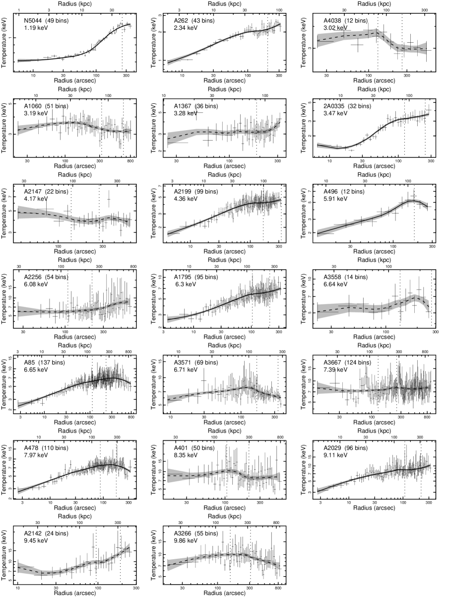
Figure 3: Projected temperature profiles and 1$\sigma$ error envelopes for each system, ordered by increasing mean temperature from top left to bottom right. The curves represent a locally-weighted fit to the data points (in log-log space). Cool-core clusters are denoted by solid lines and non cool-core clusters are plotted with dashed lines. Vertical dotted lines bracket the region 0.1–0.2 $r_{\mathrm{500}}$, within which the mean temperature is measured. The mean temperature for each cluster is indicated, as is the number of annular bins used to construct the curves.

Figure 4: Projected, finely-binned temperature profiles for the sample, split by cool core type and using an arbitrary line style to uniquely identify each system: the cluster name entries in the legends are ordered by temperature. Both plots are scaled identically in temperature and radius. Each curve represents a locally-weighted fit to the data points (in log-log space), to suppress scatter (see text for details).

The difference between CC and non-CC clusters is very clear from Fig. 4. Within the cool core, there is a remarkable consistency in shape of the temperature profile, which follow a power law with a logarithmic slope of roughly 0.3. In most clusters this behaviour appears to extend down to a few kiloparsecs — well within the central galaxy. The obvious exception to this is the coolest system, the NGC 5044 group, which exhibits a sharp break at $\sim$10 kpc, as the logarithmic slope flattens within the central galaxy. As this is the only galaxy group in the sample, this result may point to a different scaling of hot gas at small mass scales. However, this system does display evidence of multiphase gas and morphological disturbances, in the form of X-ray cavities from AGN activity as well as a cold front (Buote et al., 2003). It is therefore possible that this flattening in $T(r)$ is an atypical feature. However, we emphasize that the possibility of a flattening of $T(r)$ in the innermost core of clusters (as recently claimed by Donahue et al., 2006, for example) is not ruled out by our data, since the ‘lowess’ regression tends to mask such behaviour, by down-weighting any deviations of the innermost few points from the general trend. This disadvantage is compensated for by the clarity with which the local regression captures the underlying trend in $T(r)$, to highlight the scaling between different clusters.

Fig. 5 shows the variation in projected temperature with scaled radius. The size of the cool core region appears to be reasonably well approximated by 0.1$r_{\mathrm{500}}$— the radius of the core exclusion region used in calculating the mean cluster temperature (Section 4.1). However, any turn-over in the temperature profile at larger radius is difficult to detect, given the limited field-of-view of the main Chandra detectors. This is compounded by the fact that all but one of the CC cluster observations analysed here used the ACIS-S detector, which covers 1/4 of the area of ACIS-I. A further systematic difference is evident at smaller radii, where the profiles in Fig. 4 extend further in for CC clusters, as a consequence of the bright cool core enabling finer annular binning.

The individual deprojected scaled temperature profiles are plotted in Fig. 6, as a function of scaled radius. Here each profile has been normalized by the mean temperature of the cluster, to provide a direct comparison between systems of different mass. It is clear that there is a tight spread between the cool core clusters, which hold to an approximately power-law form, with a logarithmic slope of $\sim$0.4 (plotted as a solid line with arbitrary normalization). Conversely, the non cool-core clusters scatter around the locus of isothermality (dotted line), showing no obvious systematic variation with radius.

Motivated by the uniformity in temperature profiles displayed by the CC clusters, we have combined all the scaled data points for these systems and subjected them to a locally-weighted regression, to determine a characteristic average temperature profile. Each cluster’s deprojected temperature profile was scaled by the mean cluster temperature ($\overline{T}$) and corresponding $r_{\mathrm{500}}$. The regression was performed in log-log space, using the r project task ‘loess’, in order to provide an estimate of the error on the regression, from the scatter about the line. Each point was weighted by its inverse variance (computed using the mean asymmetric error), to improve the rejection of outliers. The same procedure was applied to the non-CC clusters, to provide a comparison. The corresponding profiles and 1$\sigma$ error envelopes for the CC and non-CC clusters are plotted in Fig. 7. The outermost point has been excluded from the mean CC and non-CC profiles plotted, in order to minimize any bias that this single point can cause at such large radius.

Figure 5: Projected, finely-binned temperature profiles for each of the clusters, scaled to $r_{\mathrm{500}}$ and labelled according to the presence of a cool core. Each curve represents a locally-weighted fit to the data points, to suppress scatter (see text for details).

Figure 6: Deprojected temperature profiles for CC and non-CC clusters, scaled by $\overline{T}$ and plotted as a function of scaled radius. Each curve represents a locally-weighted fit to the data points, to suppress scatter (see text for details).

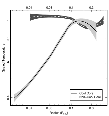
Figure 7: Mean deprojected temperature profiles for CC and non-CC clusters, scaled by $\overline{T}$ and plotted as a function of scaled radius. Each curve represents a locally-weighted fit to the data points, to suppress scatter (see text for details). The shaded regions represent the 1$\sigma$ confidence region of the fit.

The behaviour of the profiles at large radii is less certain, as indicated by the widening of the regression confidence region, resulting from the diminishing number of points. However, there is clearly a preference for a peak at $\sim$0.15 $r_{\mathrm{500}}$, followed by a decline, which is broadly consistent with previous analyses (e.g. Vikhlinin et al., 2005; Piffaretti et al., 2005; Zhang et al., 2006).

6.2 Cooling Time

A simple estimate of the susceptibility of gas to radiative cooling can be obtained by considering the timescale over which the gas can continue to lose energy at its current rate. Thus defined, the cooling time (in seconds) of a parcel of gas with volume, $V$ (in cm³), and luminosity, $L_{\mathrm{X}}$ (in erg s^-1), is given by

$$t_{\mathrm{cool}}=1.602\times 10^{-9}\times\frac{3kT\rho V\mu_{\mathrm{e}}}{2\mu L_{\mathrm{X}}},$$ (4)

where $kT$ is the deprojected gas temperature (in keV), $\rho$ is the electron number density (in cm^-3) and the constants $\mu_{\mathrm{e}}$ and $\mu$ are the mean mass per electron (1.167) and the mean molecular weight (0.593) of the gas. Profiles of cooling time as a function of scaled radius are plotted in Fig. 8, colour coded by the mean cluster temperature. As before the curves represent a locally-weighted regression to the data points. Note that the cooling time in the outermost annular bin is unknown (unlike the temperature), since the assumed volume is not well defined, which means that the gas density cannot be determined.

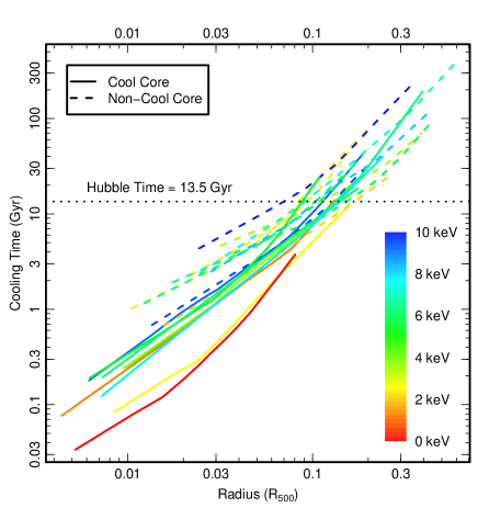
Figure 8: Gas cooling time profiles for each of the clusters, scaled to $r_{\mathrm{500}}$, labelled according to the presence of a cool core, and coloured according to the cluster mean temperature. Each curve represents a locally-weighted fit to the data points, to suppress scatter (see text for details).

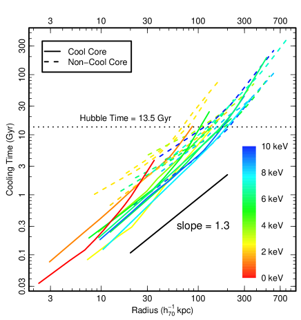
Figure 9: Same as Fig. 8, but plotted as a function of radius in kpc.

For purely bremsstrahlung X-ray emission, $t_{\mathrm{cool}}\propto\sqrt{kT}$. However, the contribution of line emission becomes significant at lower temperatures, which weakens this trend. Therefore this simple scaling has not been applied to Fig. 8, and the profiles are thus largely ordered by mean cluster temperature. Nonetheless, despite this spread in temperature, there is a clear consistency between all the profiles, with much greater similarity between CC and non-CC clusters than is seen in the gas temperature. Not surprisingly, the cool core systems have consistently lower cooling times at all radii, but they also exhibit a slightly steeper logarithmic slope than those of the non-CC clusters. While it is clear that CC clusters reach much lower values in the core, it can be seen that within $\sim$0.1$r_{\mathrm{500}}$, most non-CC clusters have rather low cooling times, falling below a Hubble time in all cases.

It can be seen in Fig. 8 that the locus corresponding to the Hubble time intersects the profiles around 0.1$r_{\mathrm{500}}$. This is the same radius used to excise any cooling-dominated flux from the mean cluster temperature estimates (Section 4.1), and also approximately corresponds to the point where the CC cluster temperature profiles reach a maximum (Fig. 7). It is apparent that even in non-CC clusters, the cooling time of gas within this radius can fall well below a Hubble time. However, the non-CC gas cooling time seems to reach a minimum level of around 1 Gyr, whereas all the CC profiles fall well below this value. To some extent this behaviour can be explained by the fact that cool core clusters permit a much finer scale spectral binning, and so their gas properties can be measured to smaller radii, where $t_{\mathrm{cool}}$ is naturally lower. Nevertheless, non-CC clusters have noticeably shallower cooling time profiles at all radii.

An alternative perspective is obtained by studying cooling time as a function of physical rather than scaled radius, as plotted in Fig. 9. Here the scatter between the profiles is actually reduced, particularly beyond $\sim$100 kpc. Moreover, the two largest outliers in Fig. 8 (the coolest two systems) lie well within the main trend, albeit with NGC 5044 showing a significantly steeper outer slope. The implication of this is that the cooling time of gas in virialized systems (either with or without a cool core) obeys a universal form across more than two orders of magnitude in radius, with relatively small scatter (a factor of $\sim$3), as found previously by Voigt & Fabian (2004) and Bauer et al. (2005). This suggests a prominent role for radiative cooling in governing cluster properties. It is not clear exactly why this should be so, but it represents an interesting challenge to theoretical models of cluster properties to account for this behaviour.

Within $\sim$100 kpc $t_{\mathrm{cool}}$ scales roughly as $r^{1.3}$, as indicated by the solid black line, which agrees with the findings of Voigt & Fabian (2004), based on a sample of 16 clusters with strong cool cores. A similar result was obtained by Bauer et al. (2005), from a sample of 38 X-ray luminous clusters at moderate redshift. Furthermore, the apparent steepening of the profiles at larger radius is also consistent with both these previous studies.

7 Discussion

It is clear that clusters can be subdivided into two distinct categories according to the presence or absence of a cool core (e.g. Peres et al., 1998; Bauer et al., 2005). How then can we explain the mixture of these types in the cluster population? Judging from our cooling time results, gas in the cores of all clusters falls well below a Hubble time (down to a least $\sim$1 Gyr). This demonstrates that the intracluster medium is certainly capable of developing a cool core in the inner regions; that it does not always do so implies the influence of some counteracting process(es).

Given the predominantly isothermal temperature profiles seen amongst the non-cool core clusters, it is natural to examine the role of cluster merging in erasing cool cores, which would tend to mix gas and smooth out thermal gradients (e.g. Fabian et al., 1984; Edge et al., 1992; Buote & Tsai, 1996). The rightmost column of Table 2 indicates which clusters show signs of merging activity, and a clear trend is apparent: 8 out of 10 ‘merger’ clusters are non-CC, leaving only 3 out of 11 non-CC clusters showing no obvious signs of merging, namely Abell 1060, Abell 4048 and Abell 3558. Of these, A1060 has a dynamically perturbed condensed core (Girardi et al., 1997) and may be a relatively recent merger cluster in which a cool core has not yet been re-established (Yamasaki et al., 2002). The CC clusters with indications of merging activity are Abell 85 and 2A0335+096. Of these, A85 clearly contains two subclusters and it appears that the cool core has survived a merger with at least one of these objects (Kempner et al., 2002). A similar event may well be occurring in 2A0335+096 (Werner et al., 2006), thus demonstrating that not all mergers are capable of destroying an existing cool core.

If merging is primarily responsible for erasing cool cores, then its impact outside this region must be relatively minor. We note that there is no evidence that the non-CC clusters are significantly hotter on average than the CC ones, (e.g. Fig. 1), based on the temperature measured within 0.1–0.2 $r_{\mathrm{500}}$ (Section 4.1); a comparison of the temperatures of the CC and non-CC clusters, using the Kolmogorov-Smirnov Test (implemented in the r project function ‘ks.test’), results in a $p$-value of 0.9195 in favour of the null hypothesis that the two sets of data are drawn from the same continuous distribution. It can be seen that the cooling time profiles of both types of cluster roughly converge beyond $\sim$0.1$r_{\mathrm{500}}$ (Fig 8). The head-on merger simulations of Gómez et al. (2002) indicate that the residual signature of a cool core may remain for up to 1–2 Gyr after a disruptive merger, before the onset of turbulence heats the gas significantly. Thus it is possible for a cool core cluster to have recently experienced a significant disruption, which could account for the presence of cool cores and merger signatures in both A85 and 2A0335+096.

Within the core, the apparent ‘floor’ value of $\sim$1 Gyr seen in the cooling time of non-CC clusters could represent the time taken to re-form a cool core. If mergers are primarily responsible for erasing cool cores, then this timescale can be linked to the characteristic timescale between such events. Specifically, the fraction of non-CC clusters would correspond to the fraction of the time between mergers that is required to re-establish a cool core. Therefore, if the $\sim$1 Gyr ‘floor’ value represents the time taken to re-form a cool core and roughly 50 per cent of the sample possess a cool core, this implies a characteristic time of $\sim$2 Gyr between mergers. By comparison, the simulations of Cohn & White (2005) indicate that, on average, clusters in their sample of 574 have experienced at least 4 large mergers since $z\sim 2$, corresponding to a lookback time of $\sim$10 Gyr. This implies a mean timescale of roughly 2.5 Gyr between mergers, which is consistent with the above figure.

Alternatively, cool cores could be disrupted by AGN-driven outflows originating in the central galaxy, which is a plausible mechanism for explaining their absence (e.g. McNamara et al., 2005; O’Sullivan et al., 2005) and is capable of mixing up gas (e.g O’Sullivan et al., 2005). However, all of the six clusters in our sample with obvious evidence of AGN-associated cavities in the ICM (marked with a ‘C’ in the rightmost column of Table 2) possess cool cores, reflecting the well established trend for cool core clusters to host central radio sources (Burns, 1990). On the other hand, AGN may well play an important role in regulating unchecked cooling in cluster cores, which is well established to be significantly suppressed (Peterson & Fabian, 2006, and references therein). If AGN activity contributes towards offsetting cooling in addition to merging, then this would impact the merger rate inferred above. Specifically, any contribution from AGN heating would require correspondingly fewer mergers, thereby increasing the timescale between such events. In that case, the value of $\sim$2 Gyr deduced above would represent a lower limit to the time between major mergers.

For purely bremsstrahlung X-ray emission the emissivity scales as $\sqrt{kT}\rho_{\mathrm{gas}}^{2}$, which in turn implies $t_{\mathrm{cool}}\propto\sqrt{kT}$. Therefore, the apparent universality of the cooling time as a function of physical radius (Fig. 9) indicates that hotter clusters must have a higher gas density (approaching $\rho_{\mathrm{gas}}\propto\sqrt{kT}$). However, a given physical radius corresponds to a smaller fraction of $r_{\mathrm{500}}$ in hotter clusters, which therefore samples gas of higher density, since $\rho_{\mathrm{gas}}$ generally increases towards the centre. Thus, even if gas at a given fraction of $r_{\mathrm{500}}$ had the same density in clusters of all masses, there would be some reduction in the scatter in $t_{\mathrm{cool}}$ plotted against physical radius compared to $r_{\mathrm{500}}$. Nevertheless, a trend for a lower gas density in groups compared to clusters has previously been reported (e.g. Sanderson et al., 2003). Furthermore, the generally good agreement found between the baryon fraction in massive clusters and the the ratio of $\Omega_{\mathrm{b}}/\Omega_{\mathrm{m}}$ (e.g. Allen et al., 2002; Sanderson & Ponman, 2003), demonstrates that it is the reduced $\rho_{\mathrm{gas}}$ in less massive systems that is anomalous.

If clusters and groups form self-similarly at any given epoch from material of constant density then radiative cooling, or indeed non-gravitational heating — operating more effectively in groups — could have acted to deplete the gas in the centres of groups, thereby lowering the density of the remaining material. However, such a process must have occurred subsequent to collapse and virialization, and so we would expect to observe evidence of systems in a intermediate state, which would register as outliers in Fig. 9. The lack of significant outliers suggests that the implied variation in gas density may already have substantially been in place prior to virialization, which implies non-self-similar accretion.

Such a scenario is consistent with models in which preheating takes places predominantly in filaments, whose linear geometry causes the energy injected to impact the density in preference to the temperature (as suggested by Ponman et al., 2003; Voit et al., 2003). Thus, the gas in the smaller filaments feeding small haloes could be ‘puffed up’ more than that in larger cluster filaments, lowering the density of material accreted onto groups. However, if this picture is correct, it points to an uncomfortable coincidence, namely that preheating of gas prior to accretion and shock heating produces virialized material of roughly constant cooling time at any given physical radius. Such an apparent conspiracy might only be resolved if some fundamental connection between preheating and cooling in haloes could be established.

7.1 Mergers, Radio Relics and Cold Fronts

Many clusters are known to possess large-scale, diffuse radio sources which are related to the intracluster medium rather than AGN (Giovannini & Feretti, 2004). Such sources emit synchrotron radiation, and are referred to as radio relics. Of the clusters in this sample, four are classified as radio relics, namely Abell 85 (Giovannini & Feretti, 2000), Abell 1367 (Gavazzi, 1978), Abell 2256 (Rottgering et al., 1994; Clarke & Ensslin, 2006) and Abell 3667 (Rottgering et al., 1997). The non-CC cluster Abell 4038 also has a radio halo similar to a relic, but this is most likely the remnant of a radio galaxy now located $\sim$18 kpc to the East of the relic (Slee et al., 2001). Similarly, Abell 2142 has a small radio halo which may originate from a single galaxy which was active in the past (Giovannini & Feretti, 2000). The generally accepted view is that genuine radio relics (i.e. much larger scale than emission from a single radio galaxy) are the product of shock waves arising from merging activity (Ensslin et al., 1998), and this picture is borne out by the fact that all four of these clusters are merger candidates. However, A85 also possesses a cool core, demonstrating that it is possible for a cool core to survive a merger energetic enough to produce a radio relic.

A related aspect is the prevalence of cold fronts in the sample, which are found in 7 of the CC clusters and 3 of the non-CC clusters. Of these 10 cold front clusters, 5 show signs of merging. Clearly cold fronts are much more common in cool core clusters (7/9) than non-CC clusters (3/11), which is consistent with the findings of Markevitch et al. (2003), who reported that roughly 70 per cent of the nearby cool core clusters in their Chandra sample of 37 contained cold fronts. A similar fraction has been found more recently from an XMM-Newton analysis of 62 clusters (Ghizzardi et al., 2005). In any case, the presence of cold fronts is certainly not incompatible with the existence of a cool core. For very relaxed clusters, like Abell 2029 and Abell 1795, cold fronts may result from the infall of small subhaloes (Ascasibar & Markevitch, 2006), rather than being caused by more substantial merging.

7.2 Properties of the Central Galaxy

Most of the clusters in this sample possess a large central galaxy which is coincident with the X-ray peak. The presence of this additional potential well is likely to impact the cluster properties in the core, so here we briefly explore the characteristics of the central galaxy. The Bautz-Morgan (BM) classification scheme (Bautz & Morgan, 1970) was devised to catalogue clusters of galaxies according to the contrast between the central galaxy and the other galaxies in the cluster (see Bahcall, 1977, for a review). There are three main categories, which are defined as follows:

Type I are clusters containing a centrally located cD galaxy

Type II are clusters where the brightest members are intermediate in appearance between cD galaxies and Virgo- or Coma-type normal giant ellipticals.

Type III are clusters containing no dominant galaxies.

Although the BM type is a subjective quantity, which is susceptible to bias (Leir & van den Bergh, 1977), it none the less provides a reasonable measure of the evolutionary state of the cluster. BM classifications are available for 17 of the 20 clusters in the sample (the 3 unclassified systems are Abell 478, NGC 5044 and 2A0335+096) and are listed in Table 2. A total of 5 out of the 6 CC clusters with a BM classification contain type I central galaxies, compared to only 3 out of 11 non-CC clusters. Moreover, the only CC cluster with a non-type I classification is an anomalous system: Abell 262 (type III) exhibits a very unusual colour magnitude relation and luminosity function, with an apparent large excess of fainter galaxies, consistent with significant contamination from a background supercluster (W. Barkhouse, Private Communication).

It is clear that BM type I clusters are more evolved than type II and III, in the sense that they are unlikely to have experienced significant recent disruption. The tendency for CC clusters to be BM type I and non-CC clusters to be types II and III is therefore consistent with the hypothesis that merger activity removes or otherwise prevents the formation of a cool core. This behaviour is consistent with the findings of Buote & Tsai (1996), who discovered a tendency for larger BM types to show evidence of global morphological disturbance in the form of a larger power ratio. Similarly, Ledlow et al. (2003) find that earlier BM types tend to have higher X-ray luminosities, consistent with their hosting cool cores, confirming the trend for cool core clusters to have an early BM type discovered by (Edge & Stewart, 1991a).

While the merger hypothesis has received support from observational studies (e.g. Allen et al., 2001) as well as earlier simulations (e.g. Ricker & Sarazin, 2001; Ritchie & Thomas, 2002), the viability of cluster merging destroying cool cores has recently been called into question (Gómez et al., 2002; Motl et al., 2004; Poole et al., 2006). The detailed investigation of Poole et al. (2006) indicate that simulations of even head-on, equal-mass mergers are incapable of disrupting an existing compact cool core, either by heating or mixing of gas. Poole et al. attribute this new development in part to a better treatment of gas cooling in their simulations, which had initially been neglected (Roettiger et al., 1997; Ricker & Sarazin, 2001). Furthermore, they incorporate empirically motivated initial conditions for their merging clusters (outlined in McCarthy et al., 2004), which result in more realistic and compact progenitor cool cores than those in the study of Ritchie & Thomas (2002), for example, who nevertheless modelled the effects of radiative cooling.

On the face of it, these new results of Poole et al. appear to rule out the possibility of cool cores ever being disrupted. However, this raises the question of why cool cores are not ubiquitous, given that the gas in all the non-CC clusters in this sample reaches cooling times as low as a few Gyr, although here are a number of possible explanations for this (see, for example the recent review of Peterson & Fabian, 2006, and references therein). Moreover, the tendency for non-CC clusters to show signs of recent disruption in the form of radio relics and a type II/III Bautz-Morgan classification is not otherwise easily understood. Finally, it must be remembered that radiative cooling and feedback are notoriously difficult processes to model in numerical simulations, and that even the most sophisticated schemes may fail to adequately capture subtle, small-scale physics of the sort that could significantly affect gas dynamics in cluster merging.

Irrespective of any causal relationship between merging activity and the presence of a cool core, the distinctive properties of the latter reinforce the notion of an intrinsic bi-modality within the cluster population. Such a conclusion has important implications for the use of scaling relations as a tool for estimating cluster properties, such as mass, since any any bi-modality would likely dominate the scatter in these relations (see O’Hara et al., 2006, for example). The extent to which this bi-modality extends to the fundamental property of mass will be addressed in a follow-up paper.

8 Conclusions

We have studied a statistically-selected sample of 20 clusters and groups of galaxies, drawn from the flux-limited catalogue of Ikebe et al. (2002), using data from the Chandra X-ray satellite. The data have been analysed using a non-parametric deprojection technique, to estimate the 3 dimensional temperature and density structure of the intracluster medium (ICM). We define a quantitative method to determine the extent to which cooling influences cluster properties: a cool core (CC) cluster is defined as one where the ratio of the mean temperature within 0.1–0.2 $r_{\mathrm{500}}$ to that within 0.1$r_{\mathrm{500}}$ exceeds unity at $>3\sigma$ significance. Accordingly we find that the sample contains 9 CC and 11 non-CC clusters.

We find that there is a clear difference between CC and non-CC clusters, with the latter exhibiting somewhat heterogeneous properties, although tending to be roughly isothermal within their inner regions. CC clusters, by contrast, display a remarkable uniformity in the shape of their inner temperature profiles. The cooling time profiles display greater uniformity across the sample, with non-CC clusters tending to possess longer cooling times at all radii, with a slightly flatter logarithmic slope. Nevertheless, even non-CC clusters have cooling times much lower than a Hubble time in all cases. This fact, together with the high incidence of merger activity found amongst the non-CC clusters, indicates that the gas mixing and shock heating that this entails may be responsible for erasing cool cores or inhibiting their formation. When the gas cooling time is plotted as a function of radius in physical units, there is a surprising decrease in the scatter between different clusters, indicative of a universal cooling time profile for gas in collapsed haloes. This result suggests that radiative cooling plays a significant role in establishing cluster properties.

References

- Allen et al. (2001) Allen S. W., Fabian A. C., Johnstone R. M., Arnaud K. A., Nulsen P. E. J., 2001, MNRAS, 322, 589
- Allen et al. (2002) Allen S. W., Schmidt R. W., Fabian A. C., 2002, MNRAS, 334, L11
- Ascasibar & Markevitch (2006) Ascasibar Y., Markevitch M., 2006, ApJ, submitted (astro-ph/0603246)
- Bîrzan et al. (2004) Bîrzan L., Rafferty D. A., McNamara B. R., Wise M. W., Nulsen P. E. J., 2004, ApJ, 607, 800
- Bahcall (1977) Bahcall N. A., 1977, ARA&A, 15, 505
- Bauer et al. (2005) Bauer F. E., Fabian A. C., Sanders J. S., Allen S. W., Johnstone R. M., 2005, MNRAS, 359, 1481
- Bautz & Morgan (1970) Bautz L. P., Morgan W. W., 1970, ApJ, 162, L149
- Blanton et al. (2004) Blanton E. L., Sarazin C. L., McNamara B. R., Clarke T. E., 2004, ApJ, 612, 817
- Buote et al. (2003) Buote D. A., Lewis A. D., Brighenti F., Mathews W. G., 2003, ApJ, 594, 741
- Buote & Tsai (1996) Buote D. A., Tsai J. C., 1996, ApJ, 458, 27
- Burns (1990) Burns J. O., 1990, AJ, 99, 14
- Clarke & Ensslin (2006) Clarke T. E., Ensslin T. A., 2006, AJ, 131, 2900
- Cohn & White (2005) Cohn J. D., White M., 2005, Astroparticle Physics, 24, 316
- Cortese et al. (2004) Cortese L., Gavazzi G., Boselli A., Iglesias-Paramo J., Carrasco L., 2004, A&A, 425, 429
- Dickey & Lockman (1990) Dickey J. M., Lockman F. J., 1990, ARA&A, 28, 215
- Donahue et al. (2006) Donahue M., Horner D. J., Cavagnolo K. W., Voit G. M., 2006, ApJ, 643, 730
- Dupke & White (2003) Dupke R., White R. E., 2003, ApJ, 583, L13
- Edge & Stewart (1991a) Edge A. C., Stewart G. C., 1991a, MNRAS, 252, 428
- Edge & Stewart (1991b) Edge A. C., Stewart G. C., 1991b, MNRAS, 252, 414
- Edge et al. (1992) Edge A. C., Stewart G. C., Fabian A. C., 1992, MNRAS, 258, 1772
- Ensslin et al. (1998) Ensslin T. A., Biermann P. L., Klein U., Kohle S., 1998, A&A, 332, 395
- Fabian et al. (1984) Fabian A. C., Nulsen P. E. J., Canizares C. R., 1984, Nature, 310, 733
- Finoguenov et al. (2001) Finoguenov A., Reiprich T. H., Böhringer H., 2001, A&A, 368, 749
- Fukazawa et al. (2004) Fukazawa Y., Makishima K., Ohashi T., 2004, PASJ, 56, 965
- Gavazzi (1978) Gavazzi G., 1978, A&A, 69, 355
- Ghizzardi et al. (2005) Ghizzardi S., Molendi S., Leccardi A., Rossetti M., 2005, preprint (astro-ph/0511445)
- Giovannini & Feretti (2000) Giovannini G., Feretti L., 2000, New Astronomy, 5, 335
- Giovannini & Feretti (2004) Giovannini G., Feretti L., 2004, Journal of Korean Astronomical Society, 37, 323
- Girardi et al. (1997) Girardi M., Escalera E., Fadda D., Giuricin G., Mardirossian F., Mezzetti M., 1997, ApJ, 482, 41
- Gómez et al. (2002) Gómez P. L., Loken C., Roettiger K., Burns J. O., 2002, ApJ, 569, 122
- Grevesse & Sauval (1998) Grevesse N., Sauval A. J., 1998, Space Science Reviews, 85, 161
- Helsdon & Ponman (2000) Helsdon S. F., Ponman T. J., 2000, MNRAS, 315, 356
- Henriksen & Tittley (2002) Henriksen M. J., Tittley E. R., 2002, ApJ, 577, 701
- Ikebe et al. (2002) Ikebe Y., Reiprich T. H., Böhringer H., Tanaka Y., Kitayama T., 2002, A&A, 383, 773
- Johnstone et al. (2002) Johnstone R. M., Allen S. W., Fabian A. C., Sanders J. S., 2002, MNRAS, 336, 299
- Kempner et al. (2002) Kempner J. C., Sarazin C. L., Ricker P. M., 2002, ApJ, 579, 236
- Ledlow et al. (2003) Ledlow M. J., Voges W., Owen F. N., Burns J. O., 2003, AJ, 126, 2740
- Leir & van den Bergh (1977) Leir A. A., van den Bergh S., 1977, ApJS, 34, 381
- Lugger (1989) Lugger P. M., 1989, ApJ, 343, 572
- Markevitch (1998) Markevitch M., 1998, ApJ, 504, 27
- Markevitch et al. (1998) Markevitch M., Forman W. R., Sarazin C. L., Vikhlinin A., 1998, ApJ, 503, 77
- Markevitch et al. (2003) Markevitch M., Vikhlinin A., Forman W. R., 2003, in Bowyer S., Hwang C.-Y., eds, Astronomical Society of the Pacific Conference Series A High Resolution Picture of the Intracluster Gas. pp 37–+
- Markevitch et al. (2001) Markevitch M., Vikhlinin A., Mazzotta P., 2001, ApJ, 562, L153
- Mazzotta et al. (2003) Mazzotta P., Edge A. C., Markevitch M., 2003, ApJ, 596, 190
- McCarthy et al. (2004) McCarthy I. G., Balogh M. L., Babul A., Poole G. B., Horner D. J., 2004, ApJ, 613, 811
- McLaughlin (1999) McLaughlin D. E., 1999, AJ, 117, 2398
- McNamara et al. (2005) McNamara B. R., Nulsen P. E. J., Wise M. W., Rafferty D. A., Carilli C., Sarazin C. L., Blanton E. L., 2005, Nature, 433, 45
- Motl et al. (2004) Motl P. M., Burns J. O., Loken C., Norman M. L., Bryan G., 2004, ApJ, 606, 635
- O’Hara et al. (2006) O’Hara T. B., Mohr J. J., Bialek J. J., Evrard A. E., 2006, ApJ, 639, 64
- O’Sullivan et al. (2005) O’Sullivan E., Vrtilek J. M., Kempner J. C., 2005, ApJ, 624, L77
- O’Sullivan et al. (2005) O’Sullivan E., Vrtilek J. M., Kempner J. C., David L. P., Houck J. C., 2005, MNRAS, 357, 1134
- Peres et al. (1998) Peres C. B., Fabian A. C., Edge A. C., Allen S. W., Johnstone R. M., White D. A., 1998, MNRAS, 298, 416
- Peterson & Fabian (2006) Peterson J. R., Fabian A. C., 2006, Phys. Rep., 427, 1
- Piffaretti et al. (2005) Piffaretti R., Jetzer P., Kaastra J. S., Tamura T., 2005, A&A, 433, 101
- Ponman et al. (2003) Ponman T. J., Sanderson A. J. R., Finoguenov A., 2003, MNRAS, 343, 331
- Poole et al. (2006) Poole G. B., Fardal M. A., Babul A., McCarthy I. G., Quinn T., Wadsley J., 2006, MNRAS, submitted
- R Development Core Team (2006) R Development Core Team 2006, R: A Language and Environment for Statistical Computing. R Foundation for Statistical Computing, Vienna, Austria
- Reiprich & Böhringer (2002) Reiprich T. H., Böhringer H., 2002, ApJ, 567, 716
- Ricker & Sarazin (2001) Ricker P. M., Sarazin C. L., 2001, ApJ, 561, 621
- Ritchie & Thomas (2002) Ritchie B. W., Thomas P. A., 2002, MNRAS, 329, 675
- Roettiger et al. (1997) Roettiger K., Loken C., Burns J. O., 1997, ApJS, 109, 307
- Rottgering et al. (1994) Rottgering H., Snellen I., Miley G., de Jong J. P., Hanisch R. J., Perley R., 1994, ApJ, 436, 654
- Rottgering et al. (1997) Rottgering H. J. A., Wieringa M. H., Hunstead R. W., Ekers R. D., 1997, MNRAS, 290, 577
- Sakelliou & Ponman (2004) Sakelliou I., Ponman T. J., 2004, MNRAS, 351, 1439
- Sanderson et al. (2005) Sanderson A. J. R., Finoguenov A., Mohr J. J., 2005, ApJ, 630, 191
- Sanderson & Ponman (2003) Sanderson A. J. R., Ponman T. J., 2003, MNRAS, 345, 1241
- Sanderson et al. (2003) Sanderson A. J. R., Ponman T. J., Finoguenov A., Lloyd-Davies E. J., Markevitch M., 2003, MNRAS, 340, 989
- Slee et al. (2001) Slee O. B., Roy A. L., Murgia M., Andernach H., Ehle M., 2001, AJ, 122, 1172
- Sun et al. (2003) Sun M., Jones C., Murray S. S., Allen S. W., Fabian A. C., Edge A. C., 2003, ApJ, 587, 619
- Sun & Murray (2002) Sun M., Murray S. S., 2002, apj, 576, 708
- Sun et al. (2002) Sun M., Murray S. S., Markevitch M., Vikhlinin A., 2002, ApJ, 565, 867
- Venturi et al. (2002) Venturi T., Bardelli S., Zagaria M., Prandoni I., Morganti R., 2002, A&A, 385, 39
- Vikhlinin et al. (2001) Vikhlinin A., Markevitch M., Murray S. S., 2001, ApJ, 551, 160
- Vikhlinin et al. (2005) Vikhlinin A., Markevitch M., Murray S. S., Jones C., Forman W., Van Speybroeck L., 2005, ApJ, 628, 655
- Voigt & Fabian (2004) Voigt L. M., Fabian A. C., 2004, MNRAS, 347, 1130
- Voit et al. (2003) Voit G. M., Balogh M. L., Bower R. G., Lacey C. G., Bryan G. L., 2003, ApJ, 593, 272
- Werner et al. (2006) Werner N., de Plaa J., Kaastra J. S., Vink J., Bleeker J. A. M., Tamura T., Peterson J. R., Verbunt F., 2006, A&A, 449, 475
- Willis et al. (2005) Willis J. P., Pacaud F., Valtchanov I., Pierre M., Ponman T., Read A., Andreon S., Altieri B., Quintana H., Dos Santos S., Birkinshaw M., Bremer M., Duc P.-A., Galaz G., Gosset E., Jones L., Surdej J., 2005, MNRAS, 363, 675
- Yamasaki et al. (2002) Yamasaki N. Y., Ohashi T., Furusho T., 2002, ApJ, 578, 833
- Zhang et al. (2006) Zhang Y. ., Boehringer H., Finoguenov A., Ikebe Y., Matsushita K., Schuecker P., Guzzo L., Collins C. A., 2006, A&A, accepted (astro-ph/0603275)