Scale dependence of the primordial spectrum from combining the three-year WMAP, Galaxy Clustering, Supernovae, and Lyman-alpha forests

Abstract

We probe the scale dependence of the primordial spectrum in the light of the three-year WMAP (WMAP3) alone and WMAP3 in combination with the other cosmological observations such as galaxy clustering and Type Ia Supernova (SNIa). We pay particular attention to the combination with the Lyman $\alpha$ (Ly$\alpha$) forest. Different from the first-year WMAP (WMAP1), WMAP3’s preference on the running of the scalar spectral index on the large scales is now fairly independent of the low CMB multipoles $\ell$. A combination with the galaxy power spectrum from the Sloan Digital Sky Survey (SDSS) prefers a negative running to larger than 2$\sigma$, regardless the presence of low $\ell$ CMB ($2\leq\ell\leq 23$) or not. On the other hand if we focus on the Power Law $\Lambda$CDM cosmology with only six parameters (matter density $\Omega_{m}h^{2}$, baryon density $\Omega_{b}h^{2}$, Hubble Constant $H_{0}$, optical depth $\tau$, the spectral index, $n_{s}$, and the amplitude, $A_{s}$, of the scalar perturbation spectrum) when we drop the low $\ell$ CMB contributions WMAP3 is consistent with the Harrison-Zel’dovich-Peebles scale-invariant spectrum ($n_{s}=1$ and no tensor contributions) at $\sim 1\sigma$. When assuming a simple power law primordial spectral index or a constant running, in case one drops the low $\ell$ contributions ($2\leq\ell\leq 23$) WMAP3 is consistent with the other observations better, such as the inferred value of $\sigma_{8}$. We also find, using a spectral shape with a minimal extension of the running spectral index model, LUQAS$+$ CROFT Ly$\alpha$ and SDSS Ly$\alpha$ exhibit somewhat different preference on the spectral shape.

PACS number(s): 98.80.Es, 98.80.Cq

I Introduction

It is commonly believed that the early Universe has experienced a stage of accelerated expansion which is known as inflation Sato:1980yn ; Guth:1980zm ; Linde:2005ht . During inflation one of the tiny patches of the very early Universe was superluminally stretched to become our observable Universe today. The theory of inflation can naturally explain why the universe is flat, homogeneous and isotropic. Inflation is driven by the potential energy of a scalar field called inflaton and its quantum fluctuations turn out to be the primordial density fluctuations which seed the observed large-scale structures (LSS) and anisotropy of the Cosmic Microwave Background (CMB) Radiation. Inflation typically ends with a period of reheating when the inflaton starts rapid oscillations and it decays into standard particles. Then the universe starts the standard hot Big Bang evolution.

Over the past decade, the theory of inflation has successfully passed several nontrivial tests. In particular, the first year Wilkinson Microwave Anisotropy Probe(WMAP) Bennett:2003bz ; Kogut:2003et ; Peiris:2003ff ; Spergel:2003cb ; Hinshaw:2003ex ; Verde:2003ey has detected a large-angle anti-correlation in the temperature-polarization cross-power spectrum, which is the signature of adiabatic superhorizon fluctuations at the time of decoupling Peiris:2003ff .

The recently released three year WMAP (WMAP3) Spergel:2006hy ; Page:2006hz ; Hinshaw:2006 ; Jarosik:2006 ; WMAP3IE has marked another milestone on the precision cosmology of CMB Radiation. The simplest six-parameter power-law $\Lambda$CDM cosmology, namely with matter density $\Omega_{m}h^{2}$, baryon density $\Omega_{b}h^{2}$, Hubble Constant $H_{0}$, optical depth $\tau$, the spectral index and amplitude of the scalar perturbation spectrum, $n_{s}$ and $A_{s}$, turn out to be in good agreement with WMAP3 together with the small-scale CMB observations such as BOOMERANG Montroy:2005yx , the Arcminute Cosmology Bolometer Array Receiver (ACBAR Kuo:2002ua ), the Cosmic Background Imager (CBI Readhead:2004gy ) and the Very Small Array(VSA Dickinson:2004yr ), LSS as measured by Two degree Field (2dF) Cole:2005sx and the Sloan Digital Sky Survey (SDSS) Tegmark:2003uf and with the Type Ia Supernova (SNIa) as measured by the Riess “gold” sample Riess:2004nr and the first year Supernova Legacy Survey (SNLS) snls . This agreement between the above “canonical” cosmological model and observations can be used to test a number of possible new physics, such as the equation of state of dark energy, neutrino masses, cosmic CPT violation, etc.

Although the temperature-temperature correlation power (TT) of WMAP3 is now cosmic-variance limited up to $\ell\sim 400$ and the third peak is now detected, the features discovered by the first year WMAP Peiris:2003ff ; Spergel:2003cb are still present: the low TT quadrupole and localized oscillating features on TT for $\ell\sim 20-40$ Hinshaw:2006 . Although the signatures of glitches on the first peak discovered by the first year WMAP have now become weaker, they do exceed the limit of cosmic variance Hinshaw:2006 . In fact, even before the release of the first year WMAP Ref. Wang:2002hf claimed oscillating primordial spectrum could lead to oscillations around the first peak of CMB TT power. These data have hence revealed many interesting detailed features which cannot be explained in the simplest version of the inflation model, and we are making much effort to construct a realistic particle physics model of inflation.

As for the shape of the primordial power spectrum, it is also noteworthy that a significant deviation has been observed by WMAP3 from the simplest Harrison-Zel’dovich-Peebles scale-invariant spectrum ($n_{s}=1$ and no tensor contributions), and that this feature is more eminent with the combination of all the currently available CMB, LSS and SNIa (dubbed the case of “All” in WMAP3IE ). On the other hand, a nontrivial negative running of the scalar spectral index $\alpha_{s}$, whose existence was studied even before WMAP epoch Feng:2003nt (for relevant study see also Lewis:2002ah ), was favored by the first-year WMAP papers Bennett:2003bz ; Peiris:2003ff ; Spergel:2003cb . But its preference was somehow diminished as corrections to the likelihood functions were made Cline:2003ve ; Efstathiou:2003tv ; Slosar:2004fr . Dramatically, the new WMAP3 data prefers again a negative running in the “All” combination WMAP3IE . If confirmed, a nonvanishing running of $\alpha_{s}$ would not only constrain inflationary cosmology significantly Feng:2003mk ; Kawasaki:2003zv ; Huang:2003zp ; Yamaguchi:2003fp ; Yamaguchi:2004tn ; Chen:2004nx ; Easther:2006tv ; Yokoyama:1998rw ; Yokoyama:1998pt , but also affect the cosmological constraint on the neutrino mass Feng:2006zj ; toappear .

In the present paper, using the Markov Chain Monte Carlo (MCMC) method, we aim to probe the scale dependence of the primordial spectrum in the light of WMAP3 alone and that in combination with the other cosmological observations from galaxy clustering and SNIa. We pay particular attention to the combination with the Lyman $\alpha$ (Ly$\alpha$) forest.

We will show that, different from the first-year WMAP (WMAP1), WMAP3’s preference on the running of the scalar spectral index on the large scales is now fairly independent of the low CMB multipoles $\ell$. We also find that a combination of WMAP3 with the galaxy power spectrum from SDSS prefers a negative running with more than 2$\sigma$, regardless of the presence of low $\ell$ CMB ($2\leq\ell\leq 23$). On the other hand, if we focus on the Power Law $\Lambda$CDM cosmology with only six parameters, we find that when one drops the low $\ell$ CMB contributions WMAP3 would be consistent with the Harrison-Zel’dovich-Peebles scale-invariant spectrum at $\sim 1\sigma$. Assuming a simple power-law primordial spectral index or a constant running, in cases one drops the low $\ell$ contributions ($2\leq\ell\leq 23$) WMAP3 is consistent with the other observations better, such as the value of $\sigma_{8}$.

On the other hand, using a spectral shape with a minimal extension of the running spectral index model, we find LUQAS$+$ CROFT Ly$\alpha$ Viel:2004bf and SDSS Ly$\alpha$ McDonald:2004xn exhibit somewhat different preference on the spectral shape, although it is difficult to draw any definite conclusion because the result depends on how we model the spectral shape.

The rest of the paper is structured as follows. In Section II we describe the method and the data. In Section III we analyze the effects of low CMB multipoles on the determination of cosmological parameters using WMAP3 Spergel:2006hy ; Page:2006hz ; Hinshaw:2006 ; Jarosik:2006 ; WMAP3IE , SNIa Riess:2004nr ; snls , 2dF Cole:2005sx and Sloan Digital Sky Survey 3-D power spectrum (SDSS P(k)) Tegmark:2003uf , LUQAS+CROFT sample of Lyman $\alpha$ Viel:2004bf and SDSS Lyman $\alpha$ sample McDonald:2004xn by global fittings using the MCMC technique. In Section IV scale dependence of fluctuations is analyzed with priors on the Hubble parameter, $\Omega_{b}h^{2}$, and the cosmic age.

Discussions and conclusions are presented in the last section.

II Method and data

To break the possible degeneracies among the variations of the current cosmological parameters, we make a global fit to the cosmological observations with the publicly available Markov Chain Monte Carlo package CosmoMC Lewis:2002ah ; IEMCMC . We assume purely adiabatic initial conditions, and impose the flatness condition motivated by inflation. Our most general parameter space is

$$\textbf{p}\equiv(\omega_{b},\omega_{c},\Theta_{S},\tau,n_{s},n^{\prime}_{s},\alpha_{s},A_{s})~{},$$ (1)

where $\omega_{b}=\Omega_{b}h^{2}$ and $\omega_{c}=\Omega_{c}h^{2}$ are the physical baryon and cold dark matter densities relative to the critical density, $\Theta_{S}$ characterizes the ratio of the sound horizon to the angular diameter distance at decoupling, $\tau$ is the optical depth and $A_{s}$ is defined as the amplitude of the primordial power spectrum at $k=0.05$ Mpc^-1. The pivot scales for $n_{s}$ and $\alpha_{s}$ are also chosen at $k=0.05$ Mpc^-1. Here $h$ is the Hubble constant in unit of 100 km s^-1 Mpc^-1. The bias factors of 2dF, SDSS and LUQAS+CROFT sample of Lyman $\alpha$ (Ly$\alpha$) as analyzed in Ref.  Viel:2004bf have been used as nuisance parameters.

For some of our simulations we have included the following priors: For $h$, we make use of the Hubble Space Telescope (HST) measurement by multiplying the likelihood function with a Gaussian centered around $h=0.72$ and with a standard deviation $\sigma=0.08$ Freedman:2000cf . We impose a weak Guassian prior on the baryon density from Big Bang nucleosynthesis (BBN) Burles:2000zk : $\Omega_{b}h^{2}=0.022\pm 0.002$ (1 $\sigma$). Simultaneously we will also use a cosmic age tophat prior as 10 Gyr$<t_{0}<$20 Gyr.

In our calculations we have taken the total likelihood to be the products of the separate likelihoods (${\bf\cal{L}}_{i}$) of CMB, LSS, SNIa and Ly$\alpha$. In other words defining $\chi_{L,i}^{2}=-2\log{\bf\cal{L}}_{i}$, we get

$$\chi^{2}_{L,total}=\chi^{2}_{L,CMB}+\chi^{2}_{L,LSS}+\chi^{2}_{L,SNIa}+\chi^{2}_{L,Ly\alpha}~{}.$$ (2)

If the likelihood function is Gaussian, $\chi^{2}_{L}$ coincides with the usual definition of $\chi^{2}$ up to an additive constant corresponding to the logarithm of the normalization factor of ${\cal L}$. In the computation of CMB we have included the three-year WMAP (WMAP3) data with the routine for computing the likelihood supplied by the WMAP team WMAP3IE . For the purpose of comparisons in some cases we also include the first-year temperature and polarization data Bennett:2003bz ; Hinshaw:2003ex with the routine for computing the likelihood supplied by the WMAP team Verde:2003ey . To be conservative but more robust, in the fittings to the 3D power spectrum of galaxies from the SDSS Tegmark:2003uf we have used the first 14 bins only, which are supposed to be well within the linear regime sdssfit . In the calculation of the likelihood from SNIa we have marginalized over the nuisance parameter DiPietro:2002cz . The supernova data we use are the “gold” set of 157 SNIa published by Riess $et$ $al$ in Ref.  Riess:2004nr and the 71 high redshift type Ia supernova discovered during the first year of the 5-year Supernova Legacy Survey (SNLS) snls , respectively. In the fittings to SNLS we have used the additional 44 nearby SNIa, as also adopted by the SNLS group snls . In order to be conservative but more robust, we did not try to combine SNLS together with the Riess sample for cosmological parameter constraints.

The Lyman-$\alpha$ forest corresponds to the Lyman-$\alpha$ absorption of photons travelling from distant quasars ($z\sim 2-4$) by the neutral hydrogen in the intergalactic medium (IGM). It is theoretically possible to infer the matter power spectrum from the Lyman-$\alpha$ forest Lesgourgues:2006nd ; Viel:2004bf ; McDonald:2004xn ; Viel:2006yh ; Seljak:2006bg . Previously Refs. Viel:2006yh ; Seljak:2006bg have made some studies on the shape of the primordial spectrum and $\sigma_{8}$ using Ly$\alpha$ data after the release of WMAP3. Here we use the LUQAS+CROFT sample of Lyman $\alpha$ as analyzed in Ref. Viel:2004bf ( dubbed V-Ly$\alpha$) and the SDSS Lyman $\alpha$ sample from Ref. McDonald:2004xn (dubbed S-Ly$\alpha$) for our study. We do not try to combine the two sets of Ly$\alpha$ simultaneously given the possibly unknown systematics of Ly$\alpha$ Lesgourgues:2006nd .

The likelihood of V-Ly$\alpha$ Viel:2004bf has been included in the publicly available package CosmoMC Lewis:2002ah ; IEMCMC , which can be used directly to probe some scale dependence of the primordial spectrum. On the other hand for S-Ly$\alpha$ analyzed in Ref. McDonald:2004xn we need to use the online C++ code IESlya1 . The package of CosmoMC being written in Fortran 90, it is not so straightforward to apply the code in Ref. IESlya1 in CosmoMC. Recently Slosar IESlya2 made a patch of SDSS Ly$\alpha$ to CosmoMC. We have corrected the patch IESlya2 after some nontrivial crosschecks and made our analysis for S-Ly$\alpha$ basing on the corrected patch.

Regarding the first-year WMAP data the E mode polarization not being directly measured, there have been simultaneously low TT multipoles and high TE multipoles Bennett:2003bz ; Kogut:2003et ; Hinshaw:2003ex . To be conservative Ref. Contaldi:2003zv used only TT data to probe the possible new physics during inflation and Ref. Dore:2003wp showed that if assuming without significant contaminations, in the general framework the observed TE amplitude on the largest scales would be in very large discrepancy with the observed TT for the concordance $\Lambda$CDM model. Moreover Bridle et al. Bridle:2003sa found that the claimed preference of a negative $\alpha_{s}$ was merely due to the lowest WMAP1 multipoles. In order to probe the sensitivity of the running to the lower multipoles we analyze the running properties using the CMB data with and without the contributions of lower multipoles which suffer from large cosmic variance Bond:1987ub .

For WMAP3 the large scale CMB data not only include the temperature power spectrum TT, but also the measurements of the polarization spectrum EE, BB and the temperature polarization spectrum TE. Given the distinctive feature of low $\ell$ CMB Efstathiou:2003tv ; Slosar:2004fr , for WMAP3 the pixel-based method has been applied to $C_{\ell}^{TT}$ for $2\leq\ell\leq 12$ and to polarization for $2\leq\ell\leq 23$ in Refs.  Spergel:2006hy ; Page:2006hz ; Hinshaw:2006 ; WMAP3IE . These large-scale components suffer from larger cosmic variance, possibly uncleaned foreground contaminations and their statistical nature is somewhat different from Gaussian. For these reasons we have tentatively prepared two different data-sets of WMAP3, one being the “normal” one with the full range TT, TE and other polarization data, the other being the truncated one where all of the components with $\ell\leq 23$ have been dropped. We analyze these two data-sets separately in various models and compare with each other. Also for a clear comparison and for the fact that WMAP1 should exhibit similar properties on low $\ell$ to WMAP3, we also truncate the TT and TE likelihood of WMAP1 at $\ell=24$. Thus for the truncated data-set essentially for both WMAP1 and WMAP3 we will use only the TT and TE CMB spectra on the truncated smaller scales. The truncated data-set, although with less amount of information, may be more conservative but more robust compared with the normal one.

While the simplest single field inflation generically predicts nearly scale-invariant primordial spectrum on the CMB relevant large scales, the inflaton would run faster in its later epoch and for the scales probed by WMAP$+$ Ly$\alpha$, an appreciable deviation from scale invariance is possibly present even in the framework of simple single-field inflation models. On the other hand, even for the simplest inflaton potentials known for a long time, the resulting primordial spectrum can be certainly more complicated than usually expected Hodges:1989dw ; Chen:2004nx ; Yokoyama:1998rw ; Yokoyama:1998pt .

Motivated by these we mainly focus on our fittings to the Power Law $\Lambda$CDM (PLCDM) Model with a constant primordial spectral index $n_{s}$ and Running Spectral Index $\Lambda$CDM (RLCDM) Model with a constant running $\alpha$. In order to see if models with more drastic scale-dependence are observationally more plausible, we also consider a Running Spectral Index $\Lambda$CDM Model with a step-like $n_{s}$ divided at $k=0.1$ Mpc^-1 (SRLCDM) as an example. In this model, we assume there is a constant primordial spectral index $n^{\prime}_{s}$ with no running for $k>0.1$ Mpc^-1. While the amplitudes of $n_{s}$ and $n^{\prime}_{s}$ are not continuous, we naturally assure the continuity of the primordial scalar spectrum $P_{s}(k)$ at 0.1 Mpc^-1.

The parameter $\sigma_{8}$, being defined as the amplitude of density fluctuations at 8 $h^{-1}$Mpc, cannot be determined by WMAP3 alone, which can probe the the shape of the primordial spectrum only up to $k\sim 0.1$ Mpc^-1 Spergel:2006hy , without extrapolating the information of the primordial spectrum to much smaller scales, except for an exotic case that the Hubble constant is anomalously small, which is certainly impossible at the first glance in the concordance cosmology. On the other hand if we assume NO prior on the shape of the primordial spectrum and reconstruct the shape of the primordial spectrum in a model independent way like Cosmic Inversion Matsumiya:2001xj ; Matsumiya:2002tx ; Kogo:2003yb ; Kogo:2004vt ; Kogo:2005qi , even the extremely exotic values of $h$ still remain possible, at least in cases we use only the CMB TT observations. In the present work we do not pursue the shape of the primordial spectrum in a model independent way and will study the cosmological implications on the shape of the primordial spectrum and the amplitude of $\sigma_{8}$ with the forementioned method.

It is believed that the secondary effects on CMB like the Sunyaev-Zel’dovich (SZ) effects and CMB lensing effects are typically very small and their effects are comparable with each other. One would take the risk of getting biased if considering only one of them Lewis:2006ma . Neglecting both of them is a plausible way in the determination of the cosmological parameters for the interest of the current paper Lewis:2006ma . Hence in the present study we have neglected both of the secondary effects.

For each regular calculation of MCMC, we run 6 independent chains comprising of 150,000-300,000 chain elements and spend thousands of CPU hours to calculate on a supercomputer. The average acceptance rate is about 40%. To get the converged results, we test the convergence of the chains by Gelman and Rubin GR92 criteria and typically get $R-1$ to be less than 0.05, which is more conservative than the recommended value $R-1<$0.1.

III Analysis of current observations with and without low multipole CMB contributions

III.1 WMAP data alone

Figure 1: CMB power spectra for the best fit Running Spectral Index $\Lambda$CDM Model to normal WMAP3 where full range of the data has been used and to the case where the $\ell\leq 23$ data of WMAP3 are not used. The dots with error bars are binned WMAP3 TT and TE data. HST, BBN and age priors have been adopted.

We start with an illustrative figure. In Fig.  1 we delineate the CMB power spectra for the best fit RLCDM Model to normal WMAP3 where the full range of the WMAP3 observational data has been useed and to the case where the $\ell\leq 23$ data of WMAP3 are not used. The dots with error bars are binned WMAP3 TT and TE data WMAP3IE . HST, BBN and age priors have been adopted. We have $\omega_{b}=0.0205$, $\omega_{c}=0.116$, $\Theta_{S}=1.038$, $\tau=0.092$, $\log[10^{10}A_{s}]$ (0.05Mpc^-1)$=3.039$, $n_{s}$(0.05Mpc^-1)$=0.856$ and $\alpha_{s}$(0.05Mpc^-1)$=-0.0634$ for the best fit case with normal WMAP3. Correspondingly for the case without small $\ell$ contributions the best fit values are $\omega_{b}=0.0190$, $\omega_{c}=0.141$, $\Theta_{S}=1.037$, $\tau=0.0403$, $\log[10^{10}A_{s}]$ (0.05Mpc^-1)$=3.005$, $n_{s}$(0.05Mpc^-1)$=0.747$ and $\alpha_{s}$(0.05Mpc^-1)$=-0.150$, respectively. The values of the minimum $\chi_{L}^{2}$ will be presented later in our Table 5. We can find that the main differences of the two results lie on scales $\ell\leq 20$. TE is relatively not as good a probe as TT, as can also be seen from the small-scale WMAP3 data.

For the simple PLCDM and RLCDM models some of the resulting cosmological parameters from WMAP3 alone are somewhat different from the previously believed concordance cosmology, namely the deviation from the scale invariant primordial spectrum and a lower $\sigma_{8}$, as well as a mild preference of the running $\alpha_{s}$. For this purpose we will investigate the possibility how such discrepancies are affected if we omit low $\ell$ contributions which suffer from relatively large cosmic variance. In this section no priors are adopted on $H_{0}$, $\Omega_{b}h^{2}$ and cosmic age.

TABLE 1. Median values and 1$\sigma$ constrains on Power Law $\Lambda$CDM Model with WMAP1 and WMAP3 and with/without $\ell\leq 23$ CMB contributions, shown together with the minimum $\chi_{L}^{2}$ values. “Normal” stands for the cases where the full range of the WMAP observational data has been adopted. NO priors have been adopted.

	WMAP1		WMAP3
No Prior	Normal	$\ell\leq 23$ dropped	Normal	$\ell\leq 23$ dropped
$\Omega_{b}h^{2}$	$0.0246^{+0.0026}_{-0.0021}$	$0.0250\pm 0.0025$	$0.0222\pm 0.0007$	$0.0223\pm 0.0010$
$\Omega_{c}h^{2}$	$0.115\pm 0.018$	$0.103^{+0.023}_{-0.022}$	$0.106\pm 0.008$	$0.104\pm 0.010$
$\tau$	$<0.449(95\%)$	$<0.488(95\%)$	$<0.139(95\%)$	$<0.293(95\%)$
$n_{s}$	$1.02^{+0.08}_{-0.06}$	$1.04\pm 0.08$	$0.955\pm 0.016$	$0.960^{+0.033}_{-0.031}$
$\sigma_{8}$	$0.949^{+0.143}_{-0.138}$	$0.939^{+0.132}_{-0.127}$	$0.762\pm 0.050$	$0.795\pm 0.065$
$H_{0}$	$75.6^{+9.8}_{-8.1}$	$80.6^{+12.5}_{-12.1}$	$73.0\pm 3.2$	$73.6\pm 4.9$
$\chi_{L}^{2}$	1429.0	1386.0	11252.6	5236.0

First we focus on the case with the WMAP data only. In Table 1 we list the median values and 1$\sigma$ constrains on PLCDM Model with WMAP1 and WMAP3 with/without $\ell\leq 23$ CMB contributions, shown together with the minimum $\chi_{L}^{2}$ values. “Normal” stands for the cases where the full range of the WMAP observational data has been adopted. For simplicity the amplitudes of the primordial spectrum $A_{s}$ have not been depicted. We should point out that the likelihood of “Normal” WMAP1 is somewhat problematic as mentioned in the previous parts of the present paper. On the other hand we are merely using it for comparison. From Table 1 we can find the improvement of precision on the determination of the cosmological parameters between WMAP1 and WMAP3. For the parameter $\tau$ only the $2\sigma$ upper bounds have been delineated. We should point out the reason that our WMAP1 normal results differ significantly from that by WMAP team in Ref. Spergel:2003cb is mainly due to the different priors on $\tau$: in our case $\tau$ is almost free while in Ref. Spergel:2003cb a stringent prior $\tau<0.3$ has been adopted. We can find dramatically for WMAP1 the constraint on $\tau$ changes very little without the presence of low $\ell$ CMB data. This can be easily understood given the fact that for WMAP1 the polarization data of EE has not been publicly available. On the other hand for WMAP3, all of the constraints have been weaker without the presence of low $\ell$ WMAP and especially for the cases of $\tau$ and $\sigma_{8}$. For WMAP3 the eminent effects of omitting $\ell$ $<$ 24 components are that $n_{s}$ is now consistent with the Harrison-Zel’dovich-Peebles scale-invariant spectrum and that the value of $\sigma_{8}$ is now nontrivially higher and less stringently constrained.

Compared with WMAP1, in WMAP3 the deviation from scale-invariance is remarkable due to better measurements of the polarization and also more sensitive measurements of the high $\ell$ TT data. We should point out our result in Table 1 indicates that at least for the relevant scales $24\leq\ell\leq 1000$, WMAP3 is consistent with the scale invariant spectrum at close to 1$\sigma$. Thus one may conclude the inconsistency of the scale-invariant spectrum claimed by WMAP3 analysis is mainly due to the low multipole components. Our constraint of WMAP3 “$\ell\leq 23$ dropped” on $\sigma_{8}$ is in remarkable agreement with the “$\Lambda$CDM + scale invariant fluctuations ($n_{s}=1$)” case by the WMAP team on the website WMAP3IE , with a considerably larger error bar. On the other hand, different from our case, the previously reported “$\Lambda$CDM $+$ primordial spectrum with sharp cutoff and linear prior” or “ $\Lambda$CDM $+$ primordial spectrum with sharp cutoff and log prior” on the website WMAP3IE reported a relatively stringent constraint on $n_{s}$ even in the presence of an additional parameter of the location of the sharp cutoff scale. The reason may be partially explained by the fact that the effect of reionization is mainly imprinted on low multipoles of polarization data, so that $\tau$ cannot be determined precisely if we omit low $\ell$ components. As a result the constraint on $n_{s}$ is also loosened as seen in Fig. 2.

Figure 2: Two dimensional posterior constraints on $n_{s}$-$\tau$ contours for Power Law $\Lambda$CDM Model with WMAP1 and WMAP3 and with/without $\ell\leq 23$ CMB contributions. The solid lines stand for 1- and 2 $\sigma$ respectively. NO priors have been adopted.

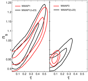
In this figure we delineate the two dimensional posterior constraints on $n_{s}$-$\tau$ contours for Power Law $\Lambda$CDM Model with WMAP1 and WMAP3 and with/without $\ell\leq 23$ CMB contributions, which correspond to the specific subspace of the likelihood surface in Table 1. The solid lines stand for 1- and 2 $\sigma$ respectively. We can see more clearly that for WMAP1 the presence of low $\ell$ CMB contributions are almost negligible but for WMAP3 the contours are significantly different, which can be easily understood from the more precise observations of WMAP3 and the $n_{s}-\tau$ degeneracy.

Figure 3: One dimensional posterior constraints on the relevant cosmological parameters for Power Law $\Lambda$CDM Model with WMAP3 data, with (red) / without (black) $\ell\leq 23$ CMB contributions. The red lines stand for WMAP3 constraints and the black for constraints with $\ell\geq 24$ WMAP. NO priors have been adopted.

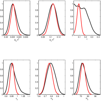
Correspondingly, in Fig. 3 we show the one dimensional posterior constraints on the relevant cosmological parameters for the PLCDM model with WMAP3 data, with/without $\ell\leq 23$ CMB contributions. The red lines stand for WMAP3 constraints and the black for constraints with $\ell\geq 24$ WMAP3. For the sake of clarity we have not depicted the WMAP1 cases. One can easily find the difference brought forth by the low $\ell$ WMAP3 temperature and polarization contributions, especially for the constraints on $\tau$, $n_{s}$ and $\sigma_{8}$.

TABLE 2. Median values and 1$\sigma$ constrains on Power Law $\Lambda$CDM Model with 2dF, SDSS, SNIa (Riess/SNLS sample) and WMAP3 (with/without $\ell\leq 23$ CMB contributions), shown together with the minimum $\chi_{L}^{2}$ values. “Normal” stands for the cases where the full range of the WMAP3 observational data has been adopted. NO priors have been adopted.

	WMAP3+LSS+SNIa(Riess)		WMAP3+LSS+SNIa(SNLS)
No Prior	Normal	$\ell\leq 23$ dropped	Normal	$\ell\leq 23$ dropped
$\Omega_{b}h^{2}$	$0.0222\pm 0.0007$	$0.0218\pm 0.0007$	$0.0223\pm 0.0007$	$0.0219\pm 0.0007$
$\Omega_{c}h^{2}$	$0.113\pm 0.005$	$0.113\pm 0.005$	$0.111\pm 0.004$	$0.111\pm 0.004$
$\tau$	$<0.122(95\%)$	$<0.167(95\%)$	$<0.128(95\%)$	$<0.191(95\%)$
$n_{s}$	$0.951\pm 0.015$	$0.937^{+0.017}_{-0.018}$	$0.953\pm 0.016$	$0.942\pm 0.019$
$\sigma_{8}$	$0.794\pm 0.035$	$0.788^{+0.047}_{-0.046}$	$0.786\pm 0.035$	$0.786^{+0.054}_{-0.052}$
$H_{0}$	$69.8\pm 1.8$	$68.9\pm 1.8$	$71.0\pm 1.8$	$70.1\pm 1.8$
$\chi_{L}^{2}$	11495.2	5476.8	11428.4	5410.8

III.2 WMAP3 data combined with LSS and SNIa

We now turn to the case LSS and SNIa are combined with CMB. Here we incorporate both 2dF Cole:2005sx and SDSS Tegmark:2003uf as for LSS data, while for SNIa due to the forementioned reason we combine in one case with the Riess “gold” sample Riess:2004nr only and in the other case with the first year SNLS snls only. First we study the PLCDM model. In Table 2 we show the median values and 1$\sigma$ constrains on the PLCDM model with 2dF, SDSS, SNIa (Riess/SNLS sample) and WMAP3 (with/without $\ell\leq 23$ CMB contributions), shown together with the minimum $\chi_{L}^{2}$ values. We can easily find that with the increased observational input, low $\ell$ CMB components lose weight for the less relevant parameters like $\Omega_{b}h^{2}$, $\Omega_{c}h^{2}$ and $H_{0}$. On the other hand the parameters like $\tau$, $n_{s}$ and $\sigma_{8}$ are nontrivially affected depending on the presence of $\ell\leq 23$ CMB contributions, because low multipole components are much affected by $\tau$, while the sensitivities of $n_{s}$ and especially $\sigma_{8}$ on the low-$\ell$ components are merely due to the fact that we are trying to fit the global shape of the power spectrum with less degrees of freedom. Compared with WMAP3 only case in Table 1 the error bars are much smaller in cases of “$\ell\leq 23$ dropped” in Table 2. Very intriguingly this leads to the fact that now the results are again inconsistent with the Harrison-Zel’dovich-Peebles scale-invariant spectrum, and in cases one drops the $\ell\leq 23$ CMB contributions $n_{s}$ is even redder (smaller than 1) than the “Normal” case. Also for the case of WMAP3+LSS+SNIa(Riess), a smaller mean central value of $\sigma_{8}$ is present without $\ell\leq 23$ CMB contributions, which is in the opposite direction compared with WMAP only case. In the left and right columns of Table 2 the determinations on the cosmological parameters are somewhat different for the case with WMAP3+LSS+SNIa(Riess) and that with WMAP3+LSS+SNIa(SNLS), but strikingly consistent at 1$\sigma$. We will address this issue in more details in the later part of the current paper.

Figure 4: Two dimensional posterior constraints on $n_{s}$-$\tau$ contours for Power Law $\Lambda$CDM Model with 2dF, SDSS, SNIa (Riess/SNLS sample) and WMAP3 (with/without $\ell\leq 23$ CMB contributions). The solid lines stand for 1- and 2 $\sigma$ respectively. NO priors have been adopted.

Figure 5: Two dimensional posterior constraints on $\sigma_{8}$-$\Omega_{m}$ contours for Power Law $\Lambda$CDM Model with 2dF, SDSS, SNIa (Riess/SNLS sample) and WMAP3 (with/without $\ell\leq 23$ CMB contributions). The solid lines stand for 1- and 2 $\sigma$ respectively. NO priors have been adopted.

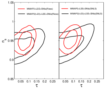
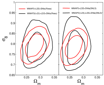
In Fig. 4 and Fig. 5 we delineate the corresponding two dimensional posterior constraints on $n_{s}$-$\tau$ contours and $\sigma_{8}$-$\Omega_{m}$ contours. The solid lines stand for 1- and 2 $\sigma$ respectively. The left panels stand for cases with WMAP3+LSS+SNIa(Riess) with/without $\ell\leq 23$ CMB contributions. The right panels show the corresponding cases with WMAP3+LSS+SNIa(SNLS). We can find that the contours in left panels are consistent but somewhat different from the right panels, and that a deviation from scale invariance is preferred. The constraints on $\sigma_{8}$ are less stringent and more consistent, however not as significant as the WMAP3 only case as shown in Table 1.

TABLE 3. Median values and 1$\sigma$ constrains on Running Spectral Index $\Lambda$CDM Model with 2dF, SDSS, SNIa (Riess/SNLS sample) and WMAP3 (with/without $\ell\leq 23$ CMB contributions), shown together with the minimum $\chi_{L}^{2}$ values. “Normal” stands for the cases where the full range of the WMAP3 observational data has been adopted. NO priors have been adopted.

	WMAP3+LSS+SNIa(Riess)		WMAP3+LSS+SNIa(SNLS)
No Prior	Normal	$\ell\leq 23$ dropped	Normal	$\ell\leq 23$ dropped
$\Omega_{b}h^{2}$	$0.0210\pm 0.0009$	$0.0208\pm 0.0010$	$0.0213\pm 0.0009$	$0.0213\pm 0.0010$
$\Omega_{c}h^{2}$	$0.116\pm 0.005$	$0.118\pm 0.005$	$0.113^{+0.005}_{-0.004}$	$0.114\pm 0.005$
$\tau$	$<0.148(95\%)$	$<0.248(95\%)$	$<0.150(95\%)$	$<0.263(95\%)$
$n_{s}$	$0.880^{+0.038}_{-0.037}$	$0.862\pm 0.049$	$0.896\pm 0.038$	$0.896\pm 0.049$
$\alpha_{s}$	$-0.0512^{+0.0251}_{-0.0254}$	$-0.0717^{+0.0425}_{-0.0419}$	$-0.0422^{+0.0257}_{-0.0258}$	$-0.0484\pm 0.0441$
$\sigma_{8}$	$0.788^{+0.036}_{-0.035}$	$0.805^{+0.068}_{-0.067}$	$0.782\pm 0.035$	$0.807^{+0.070}_{-0.068}$
$H_{0}$	$67.2\pm 2.1$	$66.5\pm 2.3$	$68.9^{+2.1}_{-2.0}$	$68.8\pm 2.3$
$\chi_{L}^{2}$	11491.4	5475.2	11425.8	5410.2

For the cosmological implications of WMAP3+LSS+SNIa now we turn to the RLCDM model. In Table 3 we delineate the median values and 1$\sigma$ constrains on Running Spectral Index $\Lambda$CDM Model with 2dF, SDSS, SNIa (Riess/SNLS sample) and WMAP3 (with/without $\ell\leq 23$ CMB contributions), shown together with the minimum $\chi_{L}^{2}$ values. Compared with Table 2 we can find that almost all of the parameters are less stringently constrained with the inclusion of $\alpha_{s}$, especially on the relevant ones like $\tau$, $n_{s}$, and $\sigma_{8}$. Due to the inclusion of $\alpha_{s}$ now all of the behaviors on the cosmological implications are again in the same direction as the WMAP3 only case in Table 1, that is, almost all of the error bars are smaller without the presence of $\ell\leq 23$ WMAP3 contributions, and a larger mean center value of $\sigma_{8}$ is present when dropping small $\ell$ CMB contributions. On the constraint on $\alpha_{s}$ itself we can find from Table 3 the case of “Normal” WMAP3+LSS+SNIa(Riess) favors a negative running of $\alpha_{s}$ to nearly $2\sigma$. For the other three cases listed a running is less favored, but still present and in some sense the preference of the negative running is fairly independent of low $\ell$ WMAP3 contributions, which will be explored in more details in the remaining part of this paper.

Figure 6: Two dimensional posterior constraints on $n_{s}$-$\alpha$ contours for Running Spectral Index $\Lambda$CDM Model with 2dF, SDSS, SNIa (Riess/SNLS sample) and WMAP3 (with/without $\ell\leq 23$ CMB contributions). The solid lines stand for 1- and 2 $\sigma$ respectively. NO priors have been adopted.

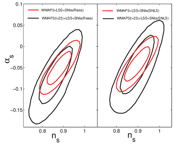
In Fig. 6 we show the corresponding two dimensional posterior constraints on $n_{s}$-$\alpha$ contours for Running Spectral Index $\Lambda$CDM Model with 2dF, SDSS, SNIa (Riess/SNLS sample) and WMAP3 (with/without $\ell\leq 23$ CMB contributions). The solid lines stand for 1- and 2 $\sigma$ respectively. We can find that in the case of dropping small $\ell$ CMB contributions the discrepancy between the left and the right panels are nontrivial and this needs to be reconsidered in more details with the accumulations of the currently ongoing SNIa projects. Also the Harrison-Zel’dovich-Peebles scale-invariant spectrum lies within the 2$\sigma$ range for the case of WMAP3+LSS+SNIa(SNLS) without small $\ell$ CMB contributions, which is different from the other three cases. It is also intriguing that in the case of “All” combination of WMAP team a negative running is preferred to more than 2$\sigma$, namely, $\alpha_{s}=-0.061\pm 0.023$ WMAP3IE . Their case of “All” differs from our analysis here regarding the following aspects: they have included small scale CMB observations and combined the SNIa data of Riess and SNLS samples simultaneously, made some detailed analysis on SDSS and 2dF bias factors and they have considered the secondary effects of SZ on WMAP3. And it is interesting to imagine the consequences without small $\ell$ CMB contributions for their case of “All”.

TABLE 4. Median values and 1$\sigma$ constrains on Power Law $\Lambda$CDM Model with WMAP3 (with/without $\ell\leq 23$ CMB contributions) combined with LUQAS+CROFT sample of Lyman $\alpha$ as analyzed in Ref. Viel:2004bf (dubbed V-Ly$\alpha$) or the SDSS Lyman $\alpha$ sample from Ref. McDonald:2004xn (dubbed S-Ly$\alpha$), shown together with the minimum $\chi_{L}^{2}$ values. “Normal” stands for the cases where the full range of the WMAP3 observational data has been adopted. NO priors have been adopted.

	WMAP3 + V-Ly$\alpha$		WMAP3 + S-Ly$\alpha$
No Prior	Normal	$\ell\leq 23$ dropped	Normal	$\ell\leq 23$ dropped
$\Omega_{b}h^{2}$	$0.0223\pm 0.0007$	$0.0223^{+0.0009}_{-0.0010}$	$0.0228\pm 0.0007$	$0.0230\pm 0.0010$
$\Omega_{c}h^{2}$	$0.110\pm 0.008$	$0.109\pm 0.009$	$0.120\pm 0.006$	$0.112\pm 0.010$
$\tau$	$<0.139(95\%)$	$<0.283(95\%)$	$<0.149(95\%)$	$<0.313(95\%)$
$n_{s}$	$0.955\pm 0.017$	$0.958\pm 0.029$	$0.964\pm 0.016$	$0.977^{+0.032}_{-0.031}$
$\sigma_{8}$	$0.787\pm 0.047$	$0.826^{+0.060}_{-0.059}$	$0.857\pm 0.024$	$0.891\pm 0.035$
$H_{0}$	$71.6^{+3.0}_{-2.9}$	$71.8\pm 4.4$	$68.8\pm 2.5$	$71.9^{+5.0}_{-4.9}$
$\chi_{L}^{2}$	11280.4	5263.2	11444.6	5425.2

Although one often takes the risks of uncontrolled systematics Lesgourgues:2006nd , Ly$\alpha$ can probe scales as small as $k\sim 1h$ Mpc ^-1 to yield the amplitude of density fluctuations $\sigma_{8}$ directly unlike the other data sets. Hence it is urged to probe the possible discrepancy between WMAP3 and Ly$\alpha$ in the determination of the cosmological parameters, especially on the value of $\sigma_{8}$. In Table 4 we delineate the median values and 1$\sigma$ constrains on Power Law $\Lambda$CDM Model with WMAP3 (with/without $\ell\leq 23$ CMB contributions) combined with V-Ly$\alpha$/ S-Ly$\alpha$, shown together with the minimum $\chi_{L}^{2}$ values. One can find again that compared with the “Normal” cases of WMAP3+Ly$\alpha$ combinations where a deviation from scale-invariance is still significant and the discrepancies on the determination of $\sigma_{8}$ are rather large among WMAP3 alone, WMAP3+V-Ly$\alpha$ and WMAP3+S-Ly$\alpha$ combinations. In cases of dropping small $\ell$ WMAP3 contributions, $n_{s}$ is nontrivially consistent with scale-invariance.

Figure 7: Two dimensional posterior constraints on $n_{s}$-$\sigma_{8}$ contours for Power Law $\Lambda$CDM Model with WMAP3 only (with/without $\ell\leq 23$ CMB contributions) or WMAP3 combined with LUQAS+CROFT sample of Lyman $\alpha$ as analyzed in Ref. Viel:2004bf (dubbed V-Ly$\alpha$) or with the SDSS Lyman $\alpha$ sample from Ref. McDonald:2004xn (dubbed S-Ly$\alpha$). The solid lines stand for 1- and 2 $\sigma$ respectively. No priors have been adopted.

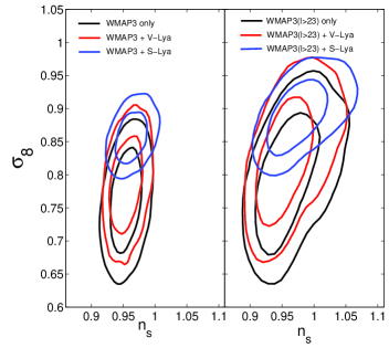
In Fig.  7 we show the corresponding two dimensional posterior constraints on $n_{s}$-$\sigma_{8}$ contours for the PLCDM model with WMAP3 (with/without $\ell\leq 23$ CMB contributions) combined with V-Ly$\alpha$/ S-Ly$\alpha$. The solid lines stand for 1- and 2 $\sigma$ respectively. In the left panel we delineate the “Normal” cases and in the right panel we show the corresponding cases where the CMB data are not used for $\ell\leq 23$. Our left panel is almost exactly the same as depicted previously in Ref. Viel:2006yh , where the discrepancies on $\sigma_{8}$ are noteworthy for the listed three kinds of different data combinations. On the other hand as shown in our right panel, in cases we neglect the low $\ell$ WMAP3 contributions, all of the contours get enlarged and these three cases are consistent with each other in a wider range of parameters.

IV Probing the scale dependence of the primordial spectrum

TABLE 5. Median values and 1$\sigma$ constrains on Running Spectral Index $\Lambda$CDM Model with WMAP1 and WMAP3 and with/without $\ell\leq 23$ CMB contributions, shown together with the minimum $\chi_{L}^{2}$ values. “Normal” stands for the cases where the full range of the WMAP observational data has been adopted. HST, BBN and age priors have been adopted.

	WMAP1		WMAP3
	Normal	$\ell\leq 23$ dropped	Normal	$\ell\leq 23$ dropped
$\Omega_{b}h^{2}$	$0.0248^{+0.0028}_{-0.0027}$	$0.0244^{+0.0029}_{-0.0031}$	$0.0209\pm 0.0010$	$0.0198^{+0.0014}_{-0.0015}$
$\Omega_{c}h^{2}$	$0.0986^{+0.0235}_{-0.0218}$	$0.106\pm 0.025$	$0.115^{+0.010}_{-0.011}$	$0.132\pm 0.019$
$\tau$	$<0.564(95\%)$	$<0.529(95\%)$	$<0.155(95\%)$	$<0.274(95\%)$
$n_{s}$	$0.985^{+0.081}_{-0.084}$	$0.996^{+0.121}_{-0.127}$	$0.876^{+0.046}_{-0.048}$	$0.789^{+0.088}_{-0.090}$
$\alpha_{s}$	$-0.0885^{+0.0474}_{-0.0466}$	$-0.0432^{+0.0891}_{-0.0886}$	$-0.0550^{+0.0307}_{-0.0317}$	$-0.135\pm 0.071$
$\sigma_{8}$	$0.936^{+0.171}_{-0.131}$	$0.939^{+0.168}_{-0.134}$	$0.782^{+0.048}_{-0.049}$	$0.831\pm 0.063$
$H_{0}$	$82.9^{+12.4}_{-13.7}$	$78.6^{+13.7}_{-13.7}$	$67.7^{+4.5}_{-4.3}$	$61.4\pm 7.0$
$\chi_{L}^{2}$	1425.4	1386.2	11249.6	5232.0

In the above investigations on the discrepancies between the implications of the current observations with and without low $\ell$ WMAP3 contributions we have adopted no priors on $H_{0}$, $\Omega_{b}h^{2}$ and cosmic age. In the following study we mainly focus on the cosmological implications on the scale dependence of the primordial spectrum, where we prefer to include the physical priors from HST, BBN and cosmic age. A running of the primordial spectrum will be studied extensively for our remaining studies.

IV.1 WMAP data alone

We also start from the WMAP only case. In Table 5 we list the median values and 1$\sigma$ constrains on Running Spectral Index $\Lambda$CDM Model with WMAP1 and WMAP3 and with/without $\ell\leq 23$ CMB contributions, shown together with the minimum $\chi_{L}^{2}$ values. As shown explicitly for WMAP1 while a negative running of $\alpha_{s}$ is close to 2$\sigma$ for the “Normal” case, no running is in full consistency with the case “$\ell\leq 23$ dropped”. Our result is consistent with the analysis by Bridle et al.  Bridle:2003sa . On the other hand, given the problematic likelihood of WMAP1 on low $\ell$ components, our analysis with “$\ell\leq 23$ dropped” should be more conservative but also more robust compared with the analysis in Ref. Bridle:2003sa . With the accumulation of the observations and better understanding on the systematics, the more precise WMAP3 shows a very different behavior on the shape of the primordial spectrum, that is, a negative running is preferred to nearly 2$\sigma$ for both of the cases with/without small $\ell$ CMB contributions. Also the parameter space for $\sigma_{8}$ is more consistent with the previously well-accepted values for the analysis of the cosmic structure formations.

Figure 8: Two dimensional posterior constraints on $n_{s}$-$\alpha_{s}$ contours for Running Spectral Index $\Lambda$CDM Model with WMAP1 and WMAP3 and with/without $\ell\leq 23$ CMB contributions. The solid lines stand for 1- and 2 $\sigma$ respectively. HST, BBN and age priors have been adopted.

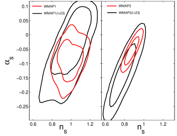
Correspondingly in Fig. 8 we show the resulting two dimensional posterior constraints on $n_{s}$-$\alpha_{s}$ contours for the RLCDM model with WMAP1 and WMAP3 and with/without $\ell\leq 23$ CMB contributions. The solid lines stand for 1- and 2 $\sigma$ respectively. While for WMAP1 even a large positive running is consistent when neglecting the small $\ell$ CMB contributions, for WMAP3 we can easily find the significantly different likelihood space where a large negative running takes the main parameter space. And also for “Normal” WMAP3 a negative running is nontrivially preferred with a higher precision compared with WMAP1, where the actual preference should be diminished if the correct likelihood functions is adopted Slosar:2004fr .

TABLE 6. Median values and 1$\sigma$ constrains on Running Spectral Index $\Lambda$CDM Model with 2dF, SDSS and WMAP3 (with/without $\ell\leq 23$ CMB contributions), shown together with the minimum $\chi_{L}^{2}$ values. “Normal” stands for the cases where the full range of the WMAP3 observational data has been adopted. HST, BBN and age priors have been adopted.

	WMAP3 + SDSS		WMAP3 + 2dF		WMAP3 + SDSS + 2dF
	Normal	$\ell\leq 23$ dropped	Normal	$\ell\leq 23$ dropped	Normal	$\ell\leq 23$ dropped
$\Omega_{b}h^{2}$	$0.0207^{+0.0010}_{-0.0009}$	$0.0194^{+0.0012}_{-0.0011}$	$0.0213\pm 0.0009$	$0.0214\pm 0.0010$	$0.0210\pm 0.0010$	$0.0205\pm 0.0012$
$\Omega_{c}h^{2}$	$0.123\pm 0.008$	$0.137\pm 0.012$	$0.111\pm 0.006$	$0.112\pm 0.007$	$0.116\pm 0.006$	$0.121\pm 0.009$
$\tau$	$<0.147(95\%)$	$<0.226(95\%)$	$<0.153(95\%)$	$<0.286(95\%)$	$<0.149(95\%)$	$<0.254(95\%)$
$n_{s}$	$0.860^{+0.043}_{-0.042}$	$0.767^{+0.067}_{-0.068}$	$0.899\pm 0.038$	$0.892^{+0.050}_{-0.052}$	$0.882^{+0.041}_{-0.042}$	$0.845^{+0.058}_{-0.069}$
$\alpha_{s}$	$-0.0655^{+0.0280}_{-0.0279}$	$-0.148^{+0.056}_{-0.059}$	$-0.0410^{+0.0256}_{-0.0258}$	$-0.0570^{+0.0467}_{-0.0477}$	$-0.0505^{+0.0274}_{-0.0271}$	$-0.0855^{+0.0550}_{-0.0551}$
$\sigma_{8}$	$0.812\pm 0.040$	$0.833^{+0.061}_{-0.060}$	$0.772^{+0.038}_{-0.036}$	$0.812\pm 0.073$	$0.788\pm 0.036$	$0.808^{+0.070}_{-0.065}$
$H_{0}$	$64.4\pm 3.2$	$59.1^{+4.2}_{-4.3}$	$69.8\pm 2.5$	$69.6\pm 3.0$	$67.5^{+2.8}_{-2.7}$	$65.4^{+3.9}_{-4.0}$
$\chi_{L}^{2}$	11267.0	5247.6	11288.8	5273.8	11307.8	5291.8

IV.2 Combination with other datasets

For a next step we consider the implications of WMAP3 in combination with LSS in great details. In Table 6 we show the median values and 1$\sigma$ constrains on the RLCDM model with 2dF, SDSS and WMAP3 (with/without $\ell\leq 23$ CMB contributions), shown together with the minimum $\chi_{L}^{2}$ values. The separate combinations of WMAP with SDSS and 2dF have also been included for the detailed investigations. The discrepancy between SDSS and 2dF is most significantly depicted in the measurement of the matter density $\Omega_{c}h^{2}$, where the tension is even more eminent in cases without low $\ell$ WMAP3 contributions. Our analysis here is consistent with the results by the WMAP group WMAP3IE . While WMAP3’s better measurements of the TT third peak help a lot on the determination of the matter density, in the concordance cosmology the measurements of $\Omega_{c}h^{2}$ from LSS are also nontrivial. The next release of SDSS power spectrum is expected to appear soon with much higher precision, the discrepancy on the matter density is hopefully to be verified or eliminated. Given the current LSS data we find that for the combination of WMAP3+SDSS the preference of running is larger than 2$\sigma$ regardless of the presence of low $\ell$ CMB. While for the WMAP3+2dF combination or that with WMAP3+2dF+SDSS, preference of a negative running is less prominent, which nevertheless does exist.

Figure 9: Two dimensional posterior constraints on $n_{s}$-$\alpha$ contours for Running Spectral Index $\Lambda$CDM Model with 2dF, SDSS and WMAP3 (with/without $\ell\leq 23$ CMB contributions). The solid lines stand for 1- and 2 $\sigma$ respectively. HST, BBN and age priors have been adopted.

Figure 10: Two dimensional posterior constraints on $\Omega_{m}$-$\sigma_{8}$ contours for Running Spectral Index $\Lambda$CDM Model with 2dF, SDSS and WMAP3 (with/without $\ell\leq 23$ CMB contributions). The solid lines stand for 1- and 2 $\sigma$ respectively. HST, BBN and age priors have been adopted.

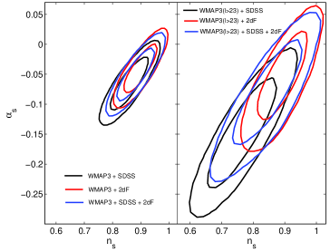
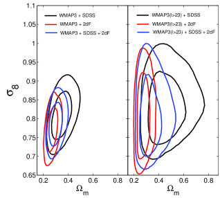
In Fig. 9 and Fig. 10 we depict the corresponding two dimensional posterior constraints on the $n_{s}$-$\alpha$ contours and on the $\Omega_{m}$-$\sigma_{8}$ contours, respectively. The solid lines stand for 1- and 2 $\sigma$ respectively. The left panels show the “Normal” constraints and the right ones show the cases where low $\ell$ WMAP3 are not used for the global fittings.

TABLE 7. Median values and 1$\sigma$ constrains on Power Law, Running Spectral Index $\Lambda$CDM Model and Running Spectral Index $\Lambda$CDM Model with step-like $n_{s}$ truncated at $k=0.1$ Mpc^-1(SRLCDM), as measured by WMAP3 in combination with LUQAS+CROFT sample of Lyman $\alpha$ as analyzed in Ref. Viel:2004bf (dubbed V-Ly$\alpha$) or the SDSS Lyman $\alpha$ sample from Ref. McDonald:2004xn (dubbed S-Ly$\alpha$), shown together with the minimum $\chi_{L}^{2}$ values. HST, BBN and age priors have been adopted.

	PLCDM			RLCDM		SRLCDM
	WMAP3 only	V-Ly$\alpha$	S-Ly$\alpha$	V-Ly$\alpha$	S-Ly$\alpha$	WMAP3 only	V-Ly$\alpha$	S-Ly$\alpha$
$10^{2}\Omega_{b}h^{2}$	$2.22\pm 0.07$	$2.24\pm 0.07$	$2.27\pm 0.06$	$2.19\pm 0.07$	$2.25\pm 0.06$	$2.12\pm 0.09$	$2.12\pm 0.09$	$2.12\pm 0.09$
$\Omega_{c}h^{2}$	$0.106^{+0.007}_{-0.008}$	$0.110\pm 0.007$	$0.120\pm 0.005$	$0.115\pm 0.008$	$0.122\pm 0.006$	$0.112\pm 0.009$	$0.118\pm 0.009$	$0.125\pm 0.006$
$\tau$	$<0.136(95\%)$	$<0.138(95\%)$	$<0.147(95\%)$	$<0.152(95\%)$	$<0.157(95\%)$	$<0.157(95\%)$	$<0.162(95\%)$	$<0.170(95\%)$
$n_{s}$	$0.953\pm 0.016$	$0.956\pm 0.015$	$0.964\pm 0.015$	$0.923^{+0.026}_{-0.027}$	$0.946\pm 0.020$	$0.887\pm 0.042$	$0.882^{+0.039}_{-0.040}$	$0.875^{+0.039}_{-0.038}$
$n_{s}^{\prime}$	$-$	$-$	$-$	$-$	$-$	$No~{}constraint$	$0.929\pm 0.090$	$0.958\pm 0.063$
$\alpha_{s}$	$-$	$-$	$-$	$-0.0268^{+0.0171}_{-0.0176}$	$-0.0154^{+0.0121}_{-0.0116}$	$-0.0487^{+0.0284}_{-0.0282}$	$-0.0552^{+0.0269}_{-0.0272}$	$-0.0635^{+0.0260}_{-0.0257}$
$\sigma_{8}$	$0.760^{+0.046}_{-0.047}$	$0.779\pm 0.045$	$0.856\pm 0.025$	$0.804^{+0.045}_{-0.047}$	$0.862\pm 0.025$	$<2.36(95\%)$	$0.818\pm 0.045$	$0.863^{+0.028}_{-0.027}$
$H_{0}$	$72.8\pm 3.0$	$71.6\pm 2.8$	$68.9\pm 2.3$	$69.4^{+3.2}_{-3.1}$	$68.0\pm 2.5$	$69.1\pm 3.7$	$67.3\pm 3.5$	$65.0\pm 2.8$
$\chi_{L}^{2}$	11252.8	11280.0	11444.6	11277.4	11443.4	11249.8	11276.6	11439.6

To measure directly the quantity of $\sigma_{8}$ one needs to include the Ly$\alpha$ observations. Now we probe the scale dependence of the primordial spectrum in the light of WMAP3 and WMAP3 in combinations with the LUQAS+CROFT sample of Lyman $\alpha$ as analyzed in Ref. Viel:2004bf (V-Ly$\alpha$) or the SDSS Lyman $\alpha$ sample from Ref. McDonald:2004xn (S-Ly$\alpha$). We investigate the three cases: PLCDM, RLCDM and SRLCDM cosmology where for SRLCDM we mean the Running Spectral Index $\Lambda$CDM Model with step-like $n_{s}$ truncated at $k=0.1$ Mpc^-1, with $n^{\prime}_{s}$ being the additionally introduced parameter which represents the spectral index on scales $k\geq 0.1$ Mpc^-1. Note in this case we have assumed a constant $n^{\prime}_{s}$. In Table 7 we list the median values and 1$\sigma$ constrains on the determinations of the relevant cosmological parameters for the three cases. For the PLCDM case a deviation from scale-invariance is present for all of the three cases in the left column of Table 7. For the RLCDM case as we are assuming a constant running on all scales, a vanishing running is consistent in either combination of WMAP3 with V-Ly$\alpha$ or S-Ly$\alpha$. For the case of SRLCDM we find many interesting implications. Because WMAP3 cannot probe scales with $k\geq 0.1$ Mpc^-1, we cannot get any constraint on the parameter $n^{\prime}_{s}$ from WMAP3 alone. And for this case we get $\sigma_{8}<2.36$ at 95% confidence level, which we will explain later in more detail. Comparing Table 7 with Table 5, we can find that the SRLCDM case of WMAP3 only is similar to that in Table 5 for the RLCDM case only, and a running is favored at less than 2$\sigma$. Interestingly for the cases of WMAP3 in combinations with V-Ly$\alpha$ or S-Ly$\alpha$, a negative running is preferred at $>2\sigma$ on scales $k\leq 0.1$ Mpc^-1 for both of the cases and the implications on $\sigma_{8}$ turn out to be more consistent. This should be relevant to the fact that the introduction of Ly$\alpha$ data changes the preference of $\Omega_{m}$ compared with WMAP3 only case, where $\Omega_{m}$ is much relevant to the TT third peak. A more intriguing aspect comes from the determination on $n^{\prime}_{s}$ for the cases in combinations with V-Ly$\alpha$ or S-Ly$\alpha$: for both cases the Harrison-Zel’dovich-Peebles scale-invariant spectrum fits well the observations on scales $k\geq 0.1$ Mpc^-1. On the other hand compared with a constant running RLCDM case, a constant negative running for $k\leq 0.1$ Mpc^-1 and nearly scale invariant spectrum for scales $k\geq 0.1$ Mpc^-1 is preferred at close to $2\sigma$ for the WMAP3+S-Ly$\alpha$ combination and similar behavior also exhibits for the WMAP3+V-Ly$\alpha$ combination, which is relatively weaker than the former case.

Figure 11: Two dimensional posterior constraints on $\Omega_{m}$-$\sigma_{8}$ contours for Power Law, Running Spectral Index $\Lambda$CDM Model and Running Spectral Index $\Lambda$CDM Model with step-like $n_{s}$ truncated at $k=0.1$ Mpc^-1 (PLCDM/RLCDM/SRLCDM), as measured by WMAP3 alone and WMAP3 in combination with the LUQAS+CROFT sample of Lyman $\alpha$ as analyzed in Ref. Viel:2004bf (dubbed V-Ly$\alpha$) or the SDSS Lyman $\alpha$ sample from Ref. McDonald:2004xn (dubbed S-Ly$\alpha$). HST, BBN and age priors have been adopted. See the text for more details.

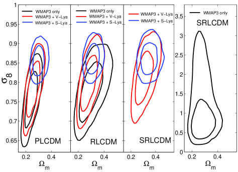
In Fig. 11 we depict the two dimensional posterior constraints on $\Omega_{m}$-$\sigma_{8}$ contours for Power Law, Running Spectral Index $\Lambda$CDM Model and Running Spectral Index $\Lambda$CDM Model with step-like $n_{s}$ truncated at $k=0.1$ Mpc^-1, as measured by WMAP3 alone and WMAP3 in combination with the LUQAS+CROFT sample of Lyman $\alpha$ as analyzed in Ref. Viel:2004bf (dubbed V-Ly$\alpha$) or the SDSS Lyman $\alpha$ sample from Ref. McDonald:2004xn (dubbed S-Ly$\alpha$). We can easily find that the discrepancy is the largest in PLCDM and as we introduce the additional parameters like a constant running and also then work in the SRLCDM framework, they gradually become consistent with each other. And for the case of SRLCDM, as $n^{\prime}_{s}$ is not constrained, the resulting constraint on $\sigma_{8}$ would definitely be extremely weak and we put the WMAP3 constraint alone on the right panel.

Figure 12: One dimensional posterior constraints on the relevant cosmological parameters for Power Law $\Lambda$CDM Model(PLCDM), Running Spectral Index $\Lambda$CDM Model(RLCDM) and Running Spectral Index $\Lambda$CDM Model with step-like $n_{s}$ truncated at $k=0.1$ Mpc^-1(SRLCDM), as measured by WMAP3 alone. The black lines stand for PLCDM, red lines for RLCDM and and the blue for SRLCDM model. HST, BBN and age priors have been adopted.

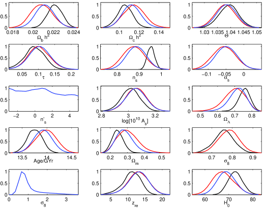
For a better study on the cosmological constraint by WMAP3 alone, in Fig. 12 we show the one dimensional posterior constraints on the relevant cosmological parameters for the PLCDM model, the RLCDM model and the SRLCDM model respectively, as measured by WMAP3 alone. The black lines stand for PLCDM, red lines for RLCDM and the blue for SRLCDM model. We should point out that although our chains have converged, our results on the SRLCDM model is much dependent on the prior adopted on the parameter $n^{\prime}_{s}$, which is easily understood given the fact that $n^{\prime}_{s}$ is unconstrained for WMAP3 alone. And a weaker prior on $n^{\prime}_{s}$ would lead to a weaker constraint on $\sigma_{8}$.

Figure 13: Resulting 2$\sigma$ posterior constraints on $n_{s}(k)$ for Running Spectral Index $\Lambda$CDM Model and Running Spectral Index $\Lambda$CDM Model with step-like $n_{s}$ truncated at $k=0.1$ Mpc^-1, as measured by WMAP3 in combination with LUQAS+CROFT sample of Lyman $\alpha$ as analyzed in Ref. Viel:2004bf and the SDSS Lyman $\alpha$ sample from Ref. McDonald:2004xn . The solid lines depict the median intervals and the dashed lines are the 2$\sigma$ limits. HST, BBN and age priors have been adopted.

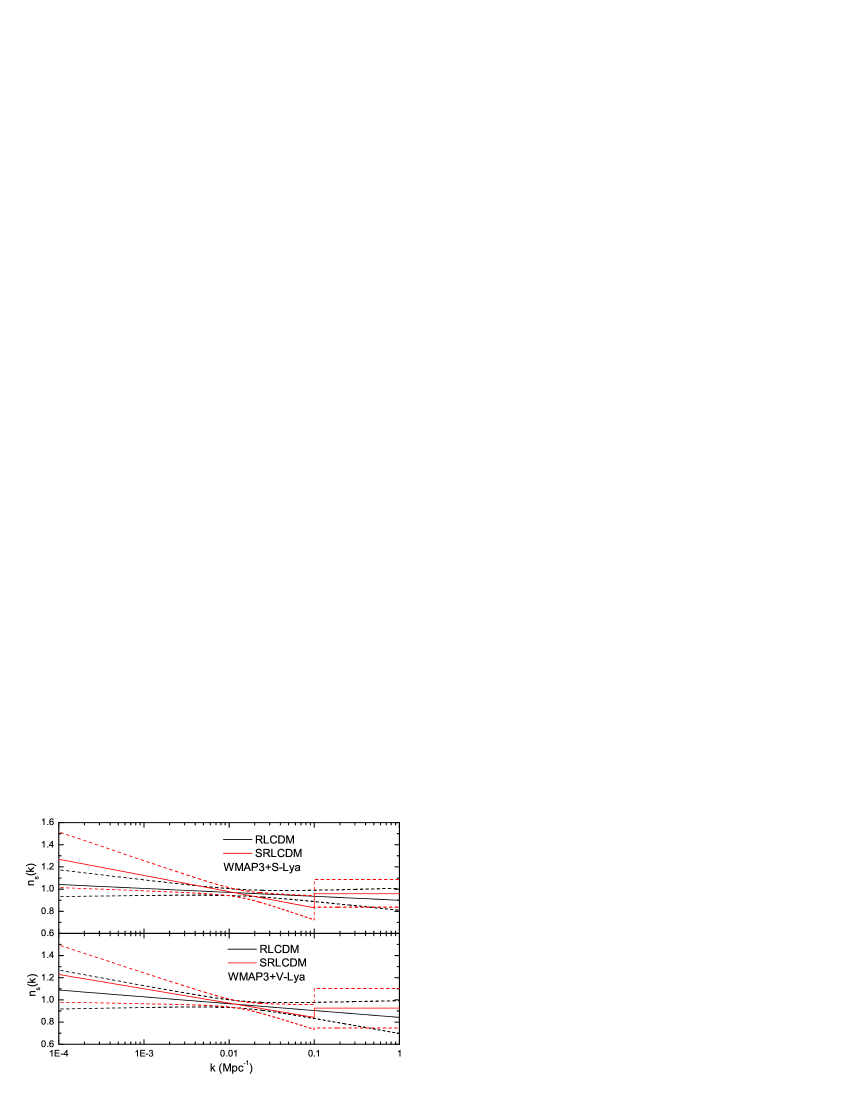
In Fig. 13 we delineate the resulting 2$\sigma$ posterior constraints on $n_{s}(k)$ for Running Spectral Index $\Lambda$CDM Model and Running Spectral Index $\Lambda$CDM Model with step-like $n_{s}$ truncated at $k=0.1$ Mpc^-1, measured by WMAP3 in combination with LUQAS+CROFT sample of Lyman $\alpha$ as analyzed in Ref. Viel:2004bf and the SDSS Lyman $\alpha$ sample from Ref. McDonald:2004xn . One can easily find the scale dependence on either of the upper or the bottom figures for the case of SRLCDM model.

V discussion and conclusion

Through our detailed investigations we have found that values of cosmological parameters obtained by MCMC change considerably depending on whether we use low multipole components of CMB or not. Currently, the WMAP team use a very large number of pixels (666+1172 pixels for low multipole temperature and polarization spectra Spergel:2006hy ; Page:2006hz ; Hinshaw:2006 ; WMAP3IE ), which may take too large a weight for the determination of the likelihood and hence cosmological parameters. This may be somewhat problematic because these low multipoles suffer from relatively large cosmic variance. On the other hand, if we incorporate low $\ell$ polarization components, the optical depth $\tau$ can be determined with a smaller ambiguity because the degeneracy between $n_{s}$ and $\tau$ is partially removed, which in turn result in a better determination of the spectral index. Hence it is difficult to conclude which approach gives more precise results.

We obtain different values of cosmological parameters with different datasets. For example, we find a very low $H_{0}$ in the combination of WMAP3 (without $\ell\leq 23$) and SDSS is rather interesting, even though we have adopted the HST prior in Table 6. Nonetheless these discrepancies are typically within 2$\sigma$ and do not imply the datasets we have used are incompatible with each other, including the differences between the Riess “gold” sample and the first year SNLS, SDSS and 2dF, or LUQAS+CROFT sample of Lyman $\alpha$ as analyzed in Ref. Viel:2004bf and the SDSS Lyman $\alpha$ sample from Ref. McDonald:2004xn

While our results as a whole support the concordance cosmology, they also indicate we are still far from being able to determine all of the six cosmological parameters with two digits’ accuracy in the context of this simple power-law $\Lambda$CDM model. Hence we should be open-minded to new physics which may be hidden in the error bars of the current observational data and continue blind analysis without any theoretical prejudices. A good example is the possible running of the spectral index, which is preferred to more than 2$\sigma$ in a number of combinations of datasets.

Acknowledgments: We acknowledge the use of the Legacy Archive for Microwave Background Data Analysis (LAMBDA). Support for LAMBDA is provided by the NASA Office of Space Science. We have performed our numerical analysis on the Shanghai Supercomputer Center (SSC). We used a modified version of CAMB Lewis:1999bs ; IEcamb which is based on CMBFAST cmbfast ; IEcmbfast . We thank Patrick Mcdonald and Anze Slosar for kind discussions regarding their online codes for SDSS Lyman alpha fittings IESlya1 ; IESlya2 . We are grateful to Kohji Yoshikawa and Ting Zhang for computational assistance. We thank Kevork Abazajian, Long-long Feng, Julien Lesgourgues, Antony Lewis, Hiranya Peiris, David Spergel, Yasushi Suto, Masahiro Takada, Max Tegmark, Matteo Viel, Yongzhong Xu, Pengjie Zhang, Xinmin Zhang and Gongbo-Zhao for helpful discussions. The work of J.Y. is supported partially by the JSPS Grant-in-Aid for Scientific Research No. 16340076 and B.F. is by the JSPS fellowship program. This work is supported in part by National Natural Science Foundation of China under Grant Nos. 90303004, 10533010 and 19925523 and by Ministry of Science and Technology of China under Grant No. NKBRSF G19990754.

Note Added: During the finalizing of our manuscript, Refs. Eriksen:2006xr ; Huffenberger:2006xx ; Bridges:2006zm ; Finelli:2006fi appeared on the arXivs which are somewhat relevant to our study.

References

- (1) K. Sato, “First Order Phase Transition Of A Vacuum And Expansion Of The Universe,” Mon. Not. Roy. Astron. Soc. 195, 467 (1981).
- (2) A. H. Guth, “The Inflationary Universe: A Possible Solution To The Horizon And Flatness Problems,” Phys. Rev. D 23, 347 (1981).
- (3) For a review of inflation, see e.g. A. D. Linde, “Particle Physics and Inflationary Cosmology,” Contemp. Concepts Phys. 5, 1 (2005) [arXiv:hep-th/0503203].
- (4) C. L. Bennett et al., “First Year Wilkinson Microwave Anisotropy Probe (WMAP) Observations: Preliminary Maps and Basic Results,” Astrophys. J. Suppl. 148, 1 (2003) [arXiv:astro-ph/0302207].
- (5) A. Kogut et al., “Wilkinson Microwave Anisotropy Probe (WMAP) First Year Observations: TE Polarization,” Astrophys. J. Suppl. 148, 161 (2003) [arXiv:astro-ph/0302213].
- (6) H. V. Peiris et al., “First year Wilkinson Microwave Anisotropy Probe (WMAP) observations: Implications for inflation,” Astrophys. J. Suppl. 148, 213 (2003) [arXiv:astro-ph/0302225].
- (7) D. N. Spergel et al. [WMAP Collaboration], “First Year Wilkinson Microwave Anisotropy Probe (WMAP) Observations: Determination of Cosmological Parameters,” Astrophys. J. Suppl. 148, 175 (2003) [arXiv:astro-ph/0302209].
- (8) G. Hinshaw et al., “First Year Wilkinson Microwave Anisotropy Probe (WMAP) Observations: Angular Power Spectrum,” Astrophys. J. Suppl. 148, 135 (2003) [arXiv:astro-ph/0302217].
- (9) L. Verde et al., “First Year Wilkinson Microwave Anisotropy Probe (WMAP) Observations: Parameter Estimation Methodology,” Astrophys. J. Suppl. 148, 195 (2003) [arXiv:astro-ph/0302218].
- (10) D. N. Spergel et al., “Wilkinson Microwave Anisotropy Probe (WMAP) Three Year Results: Implications for Cosmology,” arXiv:astro-ph/0603449.
- (11) L. Page et al., “Three Year Wilkinson Microwave Anisotropy Probe (WMAP) Observations: Polarization Analysis,” arXiv:astro-ph/0603450.
- (12) G. Hinshaw et al., “Three-Year Wilkinson Microwave Anisotropy Probe (WMAP) Observations: Temperature Analysis,” arXiv:astro-ph/0603451.
- (13) N. Jarosik et al., “Three-Year Wilkinson Microwave Anisotropy Probe (WMAP) Observations: Beam Profiles, Data Processing, Radiometer Characterization and Systematic Error Limits,” arXiv:astro-ph/0603452.
- (14) Available at http://lambda.gsfc.nasa.gov/product/map/ .
- (15) T. E. Montroy et al., “A Measurement of the CMB Spectrum from the 2003 Flight of BOOMERANG,” arXiv:astro-ph/0507514.
- (16) C. L. Kuo et al. [ACBAR collaboration], “High Resolution Observations of the CMB Power Spectrum with ACBAR,” Astrophys. J. 600, 32 (2004) [arXiv:astro-ph/0212289].
- (17) A. C. S. Readhead et al., “Extended Mosaic Observations with the Cosmic Background Imager,” Astrophys. J. 609, 498 (2004) [arXiv:astro-ph/0402359].
- (18) C. Dickinson et al., “High sensitivity measurements of the CMB power spectrum with the extended Very Small Array,” Mon. Not. Roy. Astron. Soc. 353, 732 (2004) [arXiv:astro-ph/0402498].
- (19) S. Cole et al. [The 2dFGRS Collaboration], “The 2dF Galaxy Redshift Survey: Power-spectrum analysis of the final dataset and cosmological implications,” Mon. Not. Roy. Astron. Soc. 362 (2005) 505 [arXiv:astro-ph/0501174].
- (20) M. Tegmark et al. [SDSS Collaboration], “The 3D power spectrum of galaxies from the SDSS,” Astrophys. J. 606, 702 (2004) [arXiv:astro-ph/0310725].
- (21) A. G. Riess et al. [Supernova Search Team Collaboration], “Type Ia Supernova Discoveries at From the Hubble Space Telescope: Evidence for Past Deceleration and Constraints on Dark Energy Evolution,” Astrophys. J. 607, 665 (2004) [arXiv:astro-ph/0402512].
- (22) P. Astier et al., “The Supernova Legacy Survey: Measurement of , and w from the First Year Data Set,” Astron. Astrophys. 447, 31 (2006) [arXiv:astro-ph/0510447].
- (23) X. Wang, B. Feng, M. Li, X. L. Chen and X. Zhang, “Natural inflation, Planck scale physics and oscillating primordial spectrum,” Int. J. Mod. Phys. D 14, 1347 (2005) [arXiv:astro-ph/0209242].
- (24) B. Feng, X. Gong and X. Wang, “Assessing the Effects of the Uncertainty in Reheating Energy Scale on Primordial Spectrum and CMB,” Mod. Phys. Lett. A 19, 2377 (2004) [arXiv:astro-ph/0301111].
- (25) A. Lewis and S. Bridle, “Cosmological parameters from CMB and other data: a Monte-Carlo approach,” Phys. Rev. D 66, 103511 (2002) [arXiv:astro-ph/0205436].
- (26) J. M. Cline, P. Crotty and J. Lesgourgues, “Does the small CMB quadrupole moment suggest new physics?,” JCAP 0309, 010 (2003) [arXiv:astro-ph/0304558].
- (27) See e.g. G. Efstathiou, Mon. Not. Roy. Astron. Soc. 348, 885 (2004) [arXiv:astro-ph/0310207].
- (28) See also A. Slosar, U. Seljak and A. Makarov, “Exact likelihood evaluations and foreground marginalization in low resolution WMAP data,” Phys. Rev. D 69, 123003 (2004) [arXiv:astro-ph/0403073].
- (29) B. Feng, M. z. Li, R. J. Zhang and X. m. Zhang, “An inflation model with large variations in spectral index,” Phys. Rev. D 68, 103511 (2003) [arXiv:astro-ph/0302479].
- (30) M. Kawasaki, M. Yamaguchi, and J. Yokoyama, “Inflation with a running spectral index in supergravity,” Phys. Rev. D 68, 023508 (2003) [arXiv:hep-ph/0304161].
- (31) Q. G. Huang and M. Li, “CMB power spectrum from noncommutative spacetime,” JHEP 0306, 014 (2003) [arXiv:hep-th/0304203].
- (32) M. Yamaguchi and J. Yokoyama, “Chaotic hybrid new inflation in supergravity with a running spectral index,” Phys. Rev. D 68, 123520 (2003) [arXiv:hep-ph/0307373].
- (33) M. Yamaguchi and J. Yokoyama, “Smooth hybrid inflation in supergravity with a running spectral index and early star formation,” Phys. Rev. D 70, 023513 (2004) [arXiv:hep-ph/0402282].
- (34) C.-Y. Chen, B. Feng, X.-L. Wang, and Z.-Y. Yang, “Reconstructing large running-index inflaton potentials”, Class. Quant. Grav. 21, 3223 (2004) arXiv:[astro-ph/0404419].
- (35) J. Yokoyama, “Chaotic new inflation and primordial spectrum of adiabatic fluctuations,” Phys. Rev. D 59, 107303 (1999).
- (36) J. Yokoyama, “Chaotic new inflation and formation of primordial black holes,” Phys. Rev. D 58, 083510 (1998) [arXiv:astro-ph/9802357].
- (37) R. Easther and H. Peiris, “Implications of a running spectral index for slow roll inflation,” arXiv:astro-ph/0604214.
- (38) B. Feng, J. Q. Xia, J. Yokoyama, X. Zhang and G. B. Zhao, “Weighing neutrinos in the presence of a running primordial spectral index,” arXiv:astro-ph/0605742.
- (39) B. Feng et al., to appear.
- (40) T. S. Kim, M. Viel, M. G. Haehnelt, R. F. Carswell and S. Cristiani, “The power spectrum of the flux distribution in the Lyman-alpha forest of a Large sample of UVES QSO Absorption Spectra (LUQAS),” Mon. Not. Roy. Astron. Soc. 347, 355 (2004) [arXiv:astro-ph/0308103]; R. A. C. Croft et al., “Towards a Precise Measurement of Matter Clustering: Lyman-alpha Forest Data at Redshifts 2-4,” Astrophys. J. 581, 20 (2002) [arXiv:astro-ph/0012324]; M. Viel, M. G. Haehnelt and V. Springel, “Inferring the dark matter power spectrum from the Lyman-alpha forest in high-resolution QSO absorption spectra,” Mon. Not. Roy. Astron. Soc. 354, 684 (2004) [arXiv:astro-ph/0404600].
- (41) P. McDonald et al., “The Lyman-alpha Forest Power Spectrum from the Sloan Digital Sky Survey,” Astrophys. J. Suppl. 163, 80 (2006) [arXiv:astro-ph/0405013]; P. McDonald et al., “The Linear Theory Power Spectrum from the Lyman-alpha Forest in the Sloan Digital Sky Survey,” Astrophys. J. 635, 761 (2005) [arXiv:astro-ph/0407377].
- (42) Available at http://cosmologist.info .
- (43) W. L. Freedman et al., “Final Results from the Hubble Space Telescope Key Project to Measure the Hubble Constant,” Astrophys. J. 553, 47 (2001) [arXiv:astro-ph/0012376].
- (44) S. Burles, K. M. Nollett and M. S. Turner, “Big-Bang Nucleosynthesis Predictions for Precision Cosmology,” Astrophys. J. 552, L1 (2001) [arXiv:astro-ph/0010171].
- (45) M. Tegmark et al. [SDSS Collaboration], “Cosmological parameters from SDSS and WMAP,” Phys. Rev. D 69, 103501 (2004) [arXiv:astro-ph/0310723].
- (46) For details see e.g. E. Di Pietro and J. F. Claeskens, “Quintessence models faced with future supernovae data,” Mon. Not. Roy. Astron. Soc. 341, 1299 (2003), [arXiv:astro-ph/0207332].
- (47) J. L. Prieto, A. Rest and N. B. Suntzeff, “A New Method to Calibrate the Magnitudes of Type Ia Supernovae at Maximum Light,” arXiv:astro-ph/0603407.
- (48) S. Jha, “Exploding stars, near and far,” PhD thesis, Harvard University.
- (49) J. Guy, P. Astier, S. Nobili, N. Regnault and R. Pain, “SALT: a Spectral Adaptive Light curve Template for Type Ia Supernovae,” arXiv:astro-ph/0506583.
- (50) X. F. Wang, L. F. Wang, X. Zhou, Y. Q. Lou and Z. W. Li, “A Novel Color Parameter As A Luminosity Calibrator for Type Ia Supernovae,” Astrophys. J. 620, L87 (2005) [arXiv:astro-ph/0501565].
- (51) X. F. Wang, L. F. Wang, R. Pain, X. Zhou and Z. W. Li, “Determination of the Hubble constant, the intrinsic scatter of luminosities of Type Ia SNe, and evidence for non-standard dust in other galaxies,” arXiv:astro-ph/0603392.
- (52) Available at http://sn2006.pmo.ac.cn/; X. F. Wang et al., to appear.
- (53) M. Viel, M. G. Haehnelt and A. Lewis, “The Lyman-alpha forest and WMAP year three,” arXiv:astro-ph/0604310.
- (54) U. Seljak, A. Slosar and P. McDonald, “Cosmological parameters from combining the Lyman-alpha forest with CMB, galaxy clustering and SN constraints,” arXiv:astro-ph/0604335.
- (55) See e.g. J. Lesgourgues and S. Pastor, “Massive neutrinos and cosmology,” arXiv:astro-ph/0603494.
- (56) Available at http://www.cita.utoronto.ca/pmcdonal/LyaF/ .
- (57) Available at http://www.slosar.com/aslosar/lya.html .
- (58) C. R. Contaldi, M. Peloso, L. Kofman and A. Linde, “Suppressing the lower Multipoles in the CMB Anisotropies,” JCAP 0307, 002 (2003) [arXiv:astro-ph/0303636].
- (59) O. Dore, G. P. Holder and A. Loeb, “The CMB Quadrupole in a Polarized Light,” Astrophys. J. 612 (2004) 81 [arXiv:astro-ph/0309281].
- (60) S. L. Bridle, A. M. Lewis, J. Weller and G. Efstathiou, “Reconstructing the primordial power spectrum,” Mon. Not. Roy. Astron. Soc. 342, L72 (2003) [arXiv:astro-ph/0302306].
- (61) J. R. Bond and G. Efstathiou, “The Statistics Of Cosmic Background Radiation Fluctuations,” Mon. Not. Roy. Astron. Soc. 226, 655 (1987).
- (62) H. M. Hodges, G. R. Blumenthal, L. A. Kofman and J. R. Primack, “Nonstandard Primordial Fluctuations From A Polynomial Inflaton Potential,” Nucl. Phys. B 335, 197 (1990).
- (63) M. Matsumiya, M. Sasaki and J. Yokoyama, “Cosmic inversion: Reconstructing primordial spectrum from CMB anisotropy,” Phys. Rev. D 65, 083007 (2002) [arXiv:astro-ph/0111549].
- (64) M. Matsumiya, M. Sasaki and J. Yokoyama, “Cosmic Inversion II –An iterative method for reproducing the primordial spectrum from the CMB data–,” JCAP 0302, 003 (2003) [arXiv:astro-ph/0210365].
- (65) N. Kogo, M. Matsumiya, M. Sasaki and J. Yokoyama, “Reconstructing the primordial spectrum from WMAP data by the cosmic inversion method,” Astrophys. J. 607, 32 (2004) [arXiv:astro-ph/0309662].
- (66) N. Kogo, M. Sasaki and J. Yokoyama, “Reconstructing the Primordial Spectrum with CMB Temperature and Polarization,” Phys. Rev. D 70, 103001 (2004) [arXiv:astro-ph/0409052].
- (67) N. Kogo, M. Sasaki and J. Yokoyama, “Constraining cosmological parameters by the cosmic inversion method,” Prog. Theor. Phys. 114, 555 (2005) [arXiv:astro-ph/0504471].
- (68) A. Lewis, “Observational constraints and cosmological parameters,” arXiv:astro-ph/0603753.
- (69) A. Gelman and D. Rubin, “ Inference from iterative simulation using multiple sequences,” Statistical Science 7, 457 (1992).
- (70) A. Lewis, A. Challinor and A. Lasenby, “Efficient Computation of CMB anisotropies in closed FRW models,” Astrophys. J. 538, 473 (2000) [arXiv:astro-ph/9911177].
- (71) Available at http://camb.info .
- (72) U. Seljak and M. Zaldarriaga, “A Line of Sight Approach to Cosmic Microwave Background Anisotropies,” Astrophys. J. 469, 437 (1996) [arXiv:astro-ph/9603033].
- (73) Available at http://cmbfast.org/ .
- (74) H. K. Eriksen et al., “A re-analysis of the three-year WMAP temperature power spectrum and arXiv:astro-ph/0606088.
- (75) K. M. Huffenberger, H. K. Eriksen and F. K. Hansen, “Point source power in three-year Wilkinson Microwave Anisotropy Probe data,” arXiv:astro-ph/0606538.
- (76) M. Bridges, A. N. Lasenby and M. P. Hobson, “WMAP 3-year primordial power spectrum,” arXiv:astro-ph/0607404.
- (77) F. Finelli, M. Rianna and N. Mandolesi, “WMAP Three Year Constraints on the Inflationary Expansion,” arXiv:astro-ph/0608277.