Mysteries on Universe’s Largest Observable Scales

Abstract

We review recent findings that the universe on its largest scales shows hints of the violation of statistical isotropy, in particular alignment with the geometry and direction of motion of the solar system, and missing power at scales greater than 60 degrees. We present the evidence, attempts to explain it using astrophysical, cosmological or instrumental mechanisms, and prospects for future understanding.

1 Introduction

The cosmological principle states that the universe is homogeneous and isotropic on its largest scales. The principle, introduced at the beginning of any cosmology course, is a crucial ingredient in obtaining most important results in quantitative cosmology. For example, assuming the cosmological principle, cosmic microwave background (CMB) temperature fluctuations in different directions on the sky can be averaged out, leading to accurate constraints on cosmological parameters that we have today. However, there is no fundamental reason why statistical isotropy must be obeyed by our universe. Therefore, testing the cosmological principle is one of the crucial goals of modern cosmology.

Statistical isotropy has only begun to be precision tested recently, with the advent of first large-scale maps of the cosmic microwave background anisotropy and galaxy surveys. Extraordinary full-sky maps produced by the Wilkinson Microwave Anisotropy Probe (WMAP) experiment, in particular, are revolutionizing our ability to test the isotropy of the universe on its largest scales Bennett_2003 ; Spergel_2003 ; Hinshaw_2003 ; Spergel_2006 . Stakes are set even higher with the recent discovery of dark energy that makes the universe undergo accelerated expansion. It is known that dark energy can affect the largest scales of the universe — for example, the clustering scale of dark energy may be about the horizon size today. Similarly, inflationary models can induce observable effects on the largest scales via either explicit or spontaneous violations of statistical isotropy.

2 Multipole vectors

Multipole vectors are a new basis that describes the CMB anisotropy (or more generally, any scalar function on the sky) and are particularly useful in performing tests of isotropy and alignments. CMB temperature is traditionally expressed in harmonic basis, using the spherical harmonics $Y_{\ell m}$. Copi, Huterer & Starkman (2003; CHS ) have introduced an alternative representation in terms of unit vectors

$$T_{\ell}\equiv\sum_{m}a_{\ell m}Y_{\ell m}(\theta,\phi)\approx A^{(\ell)}\prod_{i=1}^{\ell}({\hat{v}}^{(\ell,i)}\cdot{\hat{e}})\,,$$ (1)

where ${\hat{v}}^{(\ell,i)}$ is the $i^{\rm th}$ multipole vector of the $\ell^{\rm th}$ multipole. (In fact the right hand side contains terms with “angular momentum” $\ell-2$, $\ell-4$ etc.; these are subtracted by taking the appropriate traceless symmetric combination as described in CHS and CHSS .) In more technical language, Eq. (1) states the equivalence between a symmetric, traceless tensor of rank $\ell$ (middle term) and the outer product of $\ell$ unit vectors (last term). Note that the signs of all vectors can be absorbed into the sign of $A^{(\ell)}$. This representation is unique, and the right-hand side contains the familiar $2\ell+1$ degrees of freedom – two dof for each vector, plus one for $A^{(\ell)}$.

An efficient algorithm to compute the multipole vectors has been presented in CHS and is publicly available MV_code ; other algorithms have been proposed as well Katz2004 ; Weeks04 ; Helling . Interestingly, after the publication of the CHS paper CHS , Weeks Weeks04 pointed out that multipole vectors have actually first been invented by Maxwell Maxwell more than 100 years ago!

The relation between multipole vectors and the usual harmonic basis is very much the same as that between cartesian and spherical coordinates of standard geometry: both are complete bases, but specific problems are much more easily solved in one basis than the other. In particular, we and others have found that multipole vectors are particularly well suited for tests of planarity of the CMB anisotropy pattern. Moreover, a number of interesting theoretical results have been found; for example, Dennis Dennis2005 analytically computed the two-point correlation function of multipole vectors for a gaussian random, isotropic underlying field, while in Copi et al. CHSS we have studied the relation of multipole vectors to maximum angular momentum dispersion axes, maxima/minima directions, and other related quantities that have been proposed to study the CMB.

3 Alignments with the Solar System

Armed with this new representation of the CMB anisotropy, we have set out to study the morphology of CMB anisotropies on large angular scales. Prior to our work, Tegmark et al. TOH found that the octopole is planar and that the quadrupole and octopole planes are aligned. In Schwarz et al. SSHC , we have investigated the quadrupole-octopole shape and orientation using the multipole vectors. Quadrupole defines two vectors and therefore one “oriented area” vector $\hat{w}^{(\ell;i,j)}\equiv v^{(\ell,i)}\times v^{(\ell,j)}$. Octopole defines three multipole vectors and therefore three normals. Hence there are a total of four planes determined by the quadrupole and octopole.

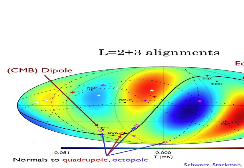
Figure 1: Quadrupole and octopole ($\ell=2$ and $3$) of the WMAP sky map in galactic coordinates, shown with the ecliptic plane, the supergalactic plane (SGP), the equinoxes and the cosmological dipole. We also show the four normals to the planes defined by vectors that describe the quadrupole and octopole temperature anisotropy; one normal is defined by the quadrupole and three by the octopole. Note that three out of four normals lie very close to both the equinoxes and the dipole direction. The probability of these alignments being accidental is about one part in a thousand. Moreover, the ecliptic plane traces out a locus of zero of the combined quadrupole and octopole over a broad swath of the sky —- neatly separating a hot spot in the northern sky from a cold spot in the south. These apparent correlations with the solar system geometry are puzzling and currently unexplained.

In Schwarz et al. we found that

• the normals to these four planes are aligned with the direction of the cosmological dipole and with the equinoxes at a level inconsistent with Gaussian random, statistically isotropic skies at $99.95$% C.L.;

• the quadrupole and octopole planes are orthogonal to the ecliptic at the $98.5$% C.L.;

• the ecliptic threads between a hot and a cold spot of the combined quadrupole and octopole map, following a node line across about $1/3$ of the sky and separating the three strong extrema from the three weak extrema of the map; this is unlikely at about the $95$% C.L.;

• the four area vectors of the quadrupole and octopole are mutually close (i.e. the quadrupole and octopole planes are aligned) at the $99.9$% C.L.

(These numbers refer to the TOH map; other maps give similar results as Table 3 of Ref. CHSS shows.) While not all of these alignments are statistically independent, they are clearly surprising, highly statistically significant (at $>99.9$% C.L.), and unexpected in the standard inflationary theory and the accepted cosmological model.

Particularly puzzling are the alignments with the solar system features. CMB anisotropy should clearly not be correlated with our local habitat. While the observed correlations seem to hint that there is contamination by a foreground or perhaps scanning strategy of the telescope, closer inspection (see the next two Sections) reveals that there is no one obvious way to explain the observed correlations.

Our studies (see CHSS ) indicate that the observed alignments are equinoctic/ecliptic ones (and/or correlated with the dipole direction), and not alignments with the Galactic plane: the alignments of the quadrupole and octopole planes with the equinox/ecliptic/dipole directions are more significant than those for the Galactic plane. This conclusion is supported by the foreground analysis (see the next Section). Moreover, it is remarkably curious that it is precisely the ecliptic alignment that has been found on somewhat smaller scales using the power spectrum analyses of statistical isotropy NS_asymmetry ; Bernui .

Finally, it is important to make sure that the results are unbiased due to unfairly chosen statistics. We have studied this issue extensively in CHSS . Two natural choices of statistics which define ordering relations on the three dot-products between the quadrupole and octopole area vectors $A_{i}$, each lying in the interval $[0,1]$, are:

$$S \equiv {1\over 3}\left(A_{1}+A_{2}+A_{3}\right),\,\,\,\,{\rm and}$$

$$T \equiv 1-{1\over 3}\left[(1-A_{1})^{2}+(1-A_{2})^{2}+(1-A_{3})^{2}\right].$$ (2)

Both $S$ and $T$ can be viewed as the suitably defined “distance” to the vertex $(A_{1},A_{2},A_{3})=(0,0,0)$. A third obvious choice, $(A_{1}^{2}+A_{2}^{2}+A_{3}^{2})/3$, is just $2S-T$. To test alignment of the quadrupole and octopole planes (or associated area vectors) we quoted the $S$ statistic numbers; $T$ gives similar results.

To test alignments of multipole planes, we define the plane as the one whose normal, $\hat{n}$, has the largest dot product with the sum of the area vectors CHSS . Since $\vec{w}_{i}\cdot\hat{n}$ is defined only up to a sign — $\vec{w}_{i}$ is headless — we take the absolute value of each dot product. Therefore, we find $\hat{n}$ that maximizes

$$\mathcal{S}\equiv\frac{1}{N_{\ell}}\sum_{i=1}^{N_{\ell}}\left|\vec{w}_{i}\cdot\hat{n}\right|,$$ (3)

where $N_{\ell}$ is the total number of area vectors considered. Alternatively, generalizing the definition in TOH , one can find the direction that maximizes the angular momentum and compare the maximal angular momentum (for the quadrupole plus octopole) with that from simulated isotropic skies CHSS

$$\hat{L}^{2}_{\ell}\equiv{\sum_{m=-\ell}^{\ell}m^{2}|a_{\ell m}|^{2}\over\ell^{2}\sum_{m=-\ell}^{\ell}\left|a_{\ell m}\right|^{2}},$$ (4)

which gives similar results as the $\mathcal{S}$ statistic for the alignment of $\ell=2$ and $\ell=3$.

4 Foregrounds

While the statistical significance of the observed vs. the Galactic alignments of the quadrupole and octopole, by itself, may not not sufficient to rule out the Galactic contamination, we have explored several lines of reasoning which suggest that Galactic foregrounds are not the cause of the alignments (see also studies by SS ; Bielewicz05 ; Abramo ).

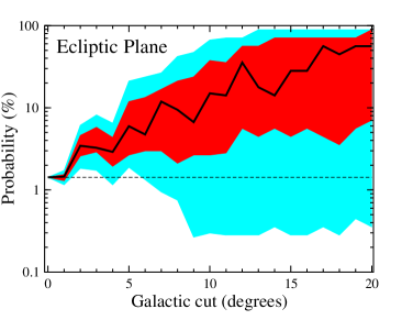
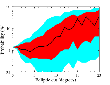
Figure 2: Quadrupole-octopole probabilities for the TOH map for an increasingly larger isolatitude cut of $\pm$(degrees shown), performed symmetrically around the Galactic plane (left panel) or the ecliptic plane (right panel). We consider the $S$ statistic probabilities applied to the ecliptic plane alignment — the solid line is the mean value, while the dark and light regions represent 68% C.L. and 95% C.L. regions, respectively, from 1000 realizations of reconstructed $a_{\ell m}$ coefficients. The dashed line denotes the probability obtained from the full-sky map, corresponding to the case of zero cut. Adopted from CHSS .

First, we have tried adding (or subtracting) known, measured Galactic contamination to WMAP maps and observing how the multipole vectors move CHSS . In the large-foreground limit, the quadrupole vectors move near the $z$-axis and the normal into the Galactic plane, while for the octopole all three normals become close to the Galactic disk at $90^{\circ}$ from the Galactic center. Therefore, as expected Galactic foregrounds lead to Galactic, and not ecliptic, correlations of the quadrupole and octopole.

Second, in CHSS , we have shown that the known Galactic foregrounds possess a multipole vector structure very different from that of the observed quadrupole and octopole. The quadrupole is nearly pure $Y_{22}$ in the frame where the $z$-axis is parallel to the dipole (or $\hat{w}^{(2,1,2)}$ or any nearly equivalent direction), while the octopole is dominantly $Y_{33}$ in the same frame. Mechanisms which produce an alteration of the microwave signal from a relatively small patch of sky — and all of the recent proposals fall into this class — are most likely to produce aligned $Y_{20}$ and $Y_{30}$ (essentially because the multipole vectors of the affected multipoles will all be parallel to each other, leading to a $Y_{\ell 0}$ in this frame).

Most of the results discussed so far have been obtained using reconstructed full-sky maps of the WMAP observations Bennett_2003 ; TOH ; LILC . Results with the reconstructed full-sky map in the presence of the sky cut is shown in Fig. (2): even with a cut of a few degrees (iso-latitude, for simplicity), the errors in the reconstructed anisotropy pattern, and the directions of multipole vectors, are too large to allow drawing quantitative conclusions about the observed alignments. Figure 2 does show, however, that the cut-sky alignment probabilities, while very uncertain, are consistent with the full-sky values. Ultimately, one will want to check for the low-$\ell$ alignments on Markov chain Monte Carlo maps, where realizations of the reconstructed the anisotropy pattern over the whole sky are based on the observations outside of the Galactic cut. While in principle straightforward (see e.g. ODwyer ), the key issue in this approach that requires considerable care is modeling of the foregrounds.

5 Quest for an explanation

Understanding the origin of CMB anomalies is clearly important, as the observed alignments of power at large scales are inconsistent with predictions of standard cosmological theory. A number of authors have attempted to explain the observed quadrupole-octopole correlations in terms of a new foreground — for example the Rees-Sciama effect Rakic06 , interstellar dust Frisch05 , local voids Inoue06 ,Ghosh . Most if not all of these proposals have a difficult time explaining the anomalies without severe fine tuning. For example, Vale Vale05 cleverly suggested that the moving lens effect, with the Great Attractor as a source, might be responsible for the extra anisotropy; however Cooray & Seto Cooray05 have argued that the lensing effect is far too small and requires too large a mass of the Attractor.

In Gordon et al. Gordon we have explored the alignment mechanisms in detail, and studied additive models where the temperature is added to the intrinsic temperature

$$T_{\rm observed}(\hat{\bf n})=T_{\rm intrinsic}(\hat{\bf n})+T_{\rm add}(\hat{\bf n})$$ (5)

where $T_{\rm add}(\hat{\bf n})$ is the additive term – perhaps contamination by a foreground, perhaps an additive instrumental or cosmological effect. We have shown that additive modulations of the CMB sky that ameliorate the alignment problems tend to worsen the overall likelihood at large scales (they still may pick up positive likelihood contribution from higher multipoles). The intuitive reason for this is that there are two penalties incurred by the additive modulation. First, since the temperature at large scales is lower than expected, one typically needs to arrange for an accidental cancellation between $T_{\rm intrinsic}$ and $T_{\rm add}$. Second, certain $a_{\ell m}$ in the dipole frame are observed to be suppressed relative to the expectation (see Table I in Ref. Gordon ) – but zero is actually the most likely value of any given $a_{\ell m}$, so likelihood with $T_{\rm intrinsic}$ is again penalized.

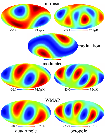
Figure 3: A realization of the multiplicative model where the quadrupole (left column) and octopole (right column) exhibit an alignment similar to WMAP. First row: intrinsic (unmodulated) sky from a Gaussian random isotropic realization. Second row (single column): the quadrupolar modulation $\propto-[1-7Y_{20}(\hat{\bf n})]$ in the dipole direction. Third row: the modulated sky of the observed CMB. Fourth row: WMAP full-sky quadrupole and octopole.

Instead, the multiplicative mechanisms, where the intrinsic temperature is multiplied by a spatially varying modulation, are more promising. As a proof of principle, we suggested a toy-model modulation

$$T_{\rm observed}(\hat{\bf n})=f\left[1+w_{2}Y_{20}(\hat{\bf n})\right]\,T_{\rm intrinsic}(\hat{\bf n}),$$ (6)

(where the modulation is a pure $Y_{20}$ along the dipole axis), we have shown that the likelihood of the WMAP data can be increased by a factor of $\exp{(16/2)}$ and, at the same time, the probability of obtaining a sky with more alignment (e.g. higher angular momentum statistic) is increased 200 times, to 45%. (Spergel et al. 2006 Spergel_2006 thereafter did a similar study, generalizing the multiplicative modulation to eight free parameters corresponding to all components of the dipole and quadrupole and finding the highest likelihood fit; see their Fig. (26)).

Finally we have considered a possibility of an imperfect instrument, where the instrumental response to the signal $T(\hat{\bf n})$ is nonlinear

$$T_{\rm observed}(\hat{\bf n})=T(\hat{\bf n})+\alpha_{2}\,T(\hat{\bf n})^{2}+\alpha_{3}\,T(\hat{\bf n})^{3}+\ldots$$ (7)

Since the biggest signal on the sky is the dipole (of order mK), leakage of about 1% (i.e. $\alpha_{1}\approx\alpha_{2}\approx 0.01$), if judiciously chosen, can produce the quadrupole and octopole that are as observed and are aligned with the dipole. Unfortunately (or fortunately!), WMAP detectors are known to be linear to much better than 1%, so this particular realization of the instrumental explanation does not work. As an aside, note that this type of explanation needs to assure that the higher multipoles are not aligned with the dipole/ecliptic, and moreover, requires essentially no intrinsic power at large scales (that is, even less than what is observed).

6 Missing angular power at large scales

Spergel et al. Spergel_2003 have found that the two point correlation function, $C(\hat{\bf n}\cdot\hat{\bf n}^{\prime})\equiv\langle T(\hat{\bf n})T(\hat{\bf n}^{\prime})\rangle$, nearly vanishes on scales greater than about 60 degrees, contrary to what the standard $\Lambda$CDM theory predicts, and in agreement with the same finding obtained from COBE data about a decade earlier DMR4 . Using the statistic

$$S_{1/2}\equiv\int_{-1}^{1/2}\left[C(\theta)\right]^{2}d(\cos\theta).$$ (8)

Spergel et al. found that only $0.15\%$ of the elements in their Markov chain of $\Lambda$CDM model CMB skies had lower values of $S_{1/2}$ than the observed sky.

We have revisited the angular two point function in the 3-yr WMAP data in Ref. Ctheta_us . We found that the two-point function computed from the various cut-sky maps shows an even stronger lack of power, now significant at the $0.03$%-$0.15$% level depending on the map used; see Fig. (4). However, we also found that, while $C(\theta)$ computed in pixel space over the unmasked sky agrees with the harmonic space calculation that uses the pseudo-$C_{\ell}$ estimator, it disagrees with the $C_{\ell}$ obtained using the maximum likelihood estimator (advocated in the 3rd year WMAP release Spergel_2006 ). The MLE-based $C_{\ell}$ lead to $C(\theta)$ that is low (according to the $S_{1/2}$ statistic) only at the 8% level. This is illustrated in the right panel of Fig. (4). We are concerned that the full-sky maximum-likelihood map making algorithm is inserting significant extra large angle power into precisely those portions of the sky where we have the least reliable information. Clearly, the definitive judgment of the large-angle power has not yet been made.

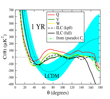
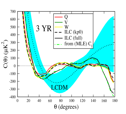
Figure 4: Two point angular correlation function, ${\mathcal{C}}(\theta)\equiv{\overline{T({\hat{e}}_{1})T({\hat{e}}_{2})}}_{\theta}$ computed in pixel space, for three different bands masked with the kp0 mask. Also shown is the correlation function for the ILC map with and without the mask, and the value expected for a statistically isotropic sky with best-fit $\Lambda$CDM cosmology together with 68% error bars. Left panel: year 1 results. Right panel: year 123 results. Even by eye, it is apparent that masked year 123 maps have $C(\theta)$ that is consistent with zero at $\theta\gtrsim 60$ deg, even more so than in year 1 maps (at the $0.03$%-$0.15$% level depending on the map used). We also show the $C(\theta)$ computed from the “official” published $C_{\ell}$, which (at $\ell<10$) are the pseudo-$C_{\ell}$ in year 1, the and MLE $C_{\ell}$ in year 123. Clearly, the maximum likelihood estimator (MLE)-based $C_{\ell}$, as well as ${\mathcal{C}}(\theta)$ computed from the full-sky ILC maps, are in significant disagreement with the angular correlation function computed from cut-sky maps.

Finally, here we note that the vanishing of power is much more apparent in real space (as in $C(\theta)$) than in multipole space (as in $C_{\ell}$). The harmonic-space quadrupole and octopole are only moderately low (e.g. ODwyer ), and it is really a range of low multipoles that conspire to make up the vanishing $C(\theta)$. Therefore, theoretical efforts to explain “low power on large scales” should focus to explain the low $C(\theta)$ at $\theta\gtrsim 60$ deg.

7 Discussion and Future Prospects

If indeed the observed $\ell=2$ and $3$ CMB fluctuations are not cosmological, one must reconsider all CMB results that rely on low $\ell$s, such as the normalization, $A$, of the primordial fluctuations and any constraint on the running $dn_{s}/d\log{k}$ of the spectral index of scalar perturbations. Moreover, the CMB-galaxy cross-correlation, which has been used to provide evidence for the Integrated Sachs-Wolfe effect and hence the existence of dark energy, also gets contributions from the lowest multipoles (though the main contribution comes from slightly smaller scales, $\ell\sim 10$). Finally, it is quite possible that the underlying physical mechanism does not cut off abruptly at the octopole, but rather affects the higher multipoles. Indeed, several pieces of evidence have been presented for anomalies at $l>3$ LandMagueijoAoE ; NS_asymmetry ; see also relevant work in Refs. Dore03 ; Chiang ; Vielva ; Freeman ; McEwen ; LandMagueijo_other ; Hajian .

So far no convincing explanation has been offered. In fact, a no-go argument has been given by Gordon et al. Gordon , reasoning that additive mechanisms for adjusting the intrinsic CMB anisotropy lead to a lower likelihood at low $\ell$ than the observed sky. Therefore, it appears that a multiplicative mechanism is at work, whether it is astrophysical, instrumental or cosmological.

While the further WMAP data (4-year, 8-year etc) is not expected to change any of the observed results, our understanding and analysis techniques are likely to improve. Much work remains to study the large-scale correlations using improved foreground treatment, accounting even for the subtle systematics, and in particular studying the time-ordered data from the spacecraft. The Planck experiment will be of great importance, as it will provide maps of the largest scales obtained using a very different experimental approach than WMAP — measuring the absolute temperature rather than temperature differences. Polarization maps, when and if available at high enough signal-to-noise at large scales (which may not be soon), will be a fantastic independent test of the alignments, and in particular each explanation for the alignments, in principle, also predicts the statistics of the polarization pattern on the sky.

The quest for an answer has whetted the appetite of cosmologists to understand the structure of the universe on its largest scales.

Acknowledgments: Topics discussed in these proceedings are a product of collaborative projects with Craig Copi, Dominik Schwarz, Glenn Starkman, Chris Gordon, Wayne Hu and Tom Crawford. The author has been supported by the NSF Astronomy and Astrophysics Postdoctoral Fellowship under Grant No. 0401066.

References

- (1) C. L. Bennett et. al., Astrophys. J. 148, S1 (2003), astro-ph/0302207.
- (2) D. N. Spergel et al. Astrophys. J. 148, S175 (2003), astro-ph/0302209.
- (3) G. Hinshaw et al. Astrophys. J. 148, S135 (2003), astro-ph/0302217.
- (4) D. N. Spergel et al. astro-ph/0603449.
- (5) C. J. Copi, D. Huterer, and G. D. Starkman, Phys. Rev. D70, 043515 (2004), astro-ph/0310511.
- (6) C. J. Copi, D. Huterer, D. J. Schwarz, and G. D. Starkman, Mon. Not. Roy. Astron. Soc. 367, 79 (2006), astro-ph/0508047.
- (7) http://www.phys.cwru.edu/projects/mpvectors/
- (8) G. Katz G. and J. Weeks, Phys. Rev. D70, 063527 (2004), astro-ph/0405631.
- (9) J.R. Weeks, astro-ph/0412231.
- (10) R.C. Helling, P. Schupp and T. Tesileanu, astro-ph/0603594.
- (11) J.C. Maxwell, “A Treatise on Electricity and Magnetism”, Clarendon Press, London, 1891
- (12) M. R. Dennis, J. Phys. A: Math. Gen. 38, 1653 (2005).
- (13) M. Tegmark, A. de Oliveira-Costa and A. J. S. Hamilton, Phys. Rev. D 68, 123523 (2003), astro-ph/0302496.
- (14) D. J. Schwarz, G. D. Starkman, D. Huterer, and C. J. Copi, Phys. Rev. Lett. 93, 221301 (2004), astro-ph/0403353.
- (15) H. K. Eriksen, F. K. Hansen, A. J. Banday, K. M. Gorski, and P. B. Lilje, Astrophys. J. 605, 14 (2004); 609, 1198 (2004) [Erratum], astro-ph/0307507; F.K. Hansen, A.J. Banday and K.M. Gorski, Mon. Not. Roy. Astron. Soc. 354, 641 (2004).
- (16) A. Bernui, B. Mota, M.J. Reboucas, and R. Tavakol, astro-ph/0511666; A. Bernui et al., astro-ph/0601593
- (17) A. Slosar and U. Seljak, Phys. Rev. D70, 083002 (2004), astro-ph/0404567.
- (18) P. Bielewicz, H.K. Eriksen, A.J. Banday, K.M. Górski and P.B. Lilje, Astrophys. J. 635, 750 (2005), astro-ph/0507186
- (19) L.R. Abramo et al., astro-ph/0604346; L.R. Abramo, S. Sodre and A. Wuensche, astro-ph/0605269.
- (20) H. K. Eriksen, A. J. Banday, K. M. Gorski, and P. B. Lilje, Astrophys. J. 612, 633 (2004), astro-ph/0403098.
- (21) I.J. O’Dwyer et al., Astrophys. J. 617, L99 (2004), astro-ph/0407027.
- (22) K. Land and J. Magueijo, Mon. Not. Roy. Astron. Soc. 362, L16 (2005), astro-ph/0407081; Phys. Rev. Lett. 95, 071301 (2005), astro-ph/0502237;
- (23) A. Rakić, S. Räsänen and D. J. Schwarz, Mon. Not. Roy. Astron. Soc. 369, L27 (2006), astro-ph/0601445.
- (24) P. C. Frisch, Astrophys. J. 632, L143 (2005), astro-ph/0506293.
- (25) K. T. Inoue and J. Silk, astro-ph/0602478.
- (26) T. Ghosh, A. Hajian and T. Souradeep, astro-ph/0604279.
- (27) C. Vale, astro-ph/0509039.
- (28) A. Cooray and N. Seto, JCAP 0512, 004 (2005), astro-ph/0510137.
- (29) C. Gordon, W. Hu, D. Huterer and T. Crawford, Phys. Rev. D 72, 103002 (2005), astro-ph/0509301.
- (30) G. Hinshaw et. al., Astrophys. J. 464, L25 (1996), astro-ph/9601061.
- (31) C. J. Copi, D. Huterer, D. J. Schwarz, and G. D. Starkman, Phys. Rev. D, submitted, astro-ph/0605135.
- (32) O. Dore, G. P. Holder, and A. Loeb, Astrophys. J. 612, 81 (2004), astro-ph/0309281.
- (33) L. Y. Chiang, P. D. Naselsky, O. V. Verkhodanov and M. J. Way, Astrophys. J. 590, L65 (2003), astro-ph/0303643; P. Naselsky, L. Y. Chiang, P. Olesen and I. Novikov, Phys. Rev. D 72, 063512 (2005), astro-ph/0505011.
- (34) P. Vielva, E. Martinez-Gonzalez, R. B. Barreiro, J. L. Sanz, and L. Cayon, Astrophys. J. 609, 22 (2004), astro-ph/0310273; M. Cruz, E. Martinez-Gonzalez, P. Vielva and L. Cayon, Mon. Not. Roy. Astron. Soc. 356, 29 (2005), astro-ph/0405341; Y. Wiaux, P. Vielva, E. Martinez-Gonzalez and P. Vandergheynst, Phys. Rev. Lett. 96, 151303 (2006), astro-ph/0603367.
- (35) P. E. Freeman, C. R. Genovese, C. J. Miller, R. C. Nichol, and L. Wasserman, Astrophys. J. 638, 1 (2006), astro-ph/0510406.
- (36) J.D. McEwen, M.P. Hobson, A.N. Lasenby and D.J. Mortlock, Mon. Not. Roy. Astron. Soc. 359, 1583 (2005), astro-ph/0406604.
- (37) K. Land and J. Magueijo, Mon. Not. Roy. Astron. Soc. 362, 838 (2005), astro-ph/0502574; K. Land and J. Magueijo, Phys. Rev. D 72, 101302 (2005), astro-ph/0507289.
- (38) A. Hajian, T. Souradeep and N. Cornish, Astrophys. J. 618, L63 (2004); A. Hajian and T. Souradeep, astro-ph/0501001; S. Basak, A. Hajian and T. Souradeep, Phys. Rev. D 74, 021301 (2006); A. Hajian and T. Souradeep, astro-ph/0607153.