The Influence of Magnetic Field on Oscillations in the Solar Chromosphere

Abstract

Two sequences of solar images obtained by the Transition Region and Coronal Explorer in three UV passbands are studied using wavelet and Fourier analysis and compared to the photospheric magnetic flux measured by the Michelson Doppler Interferometer on the Solar Heliospheric Observatory to study wave behaviour in differing magnetic environments. Wavelet periods show deviations from the theoretical cutoff value and are interpreted in terms of inclined fields. The variation of wave speeds indicates that a transition from dominant fast–magnetoacoustic waves to slow modes is observed when moving from network into plage and umbrae. This implies preferential transmission of slow modes into the upper atmosphere, where they may lead to heating or be detected in coronal loops and plumes.

1. INTRODUCTION

It has been believed for over forty years that oscillatory motions play an important role in the outer solar atmosphere (Leighton et al., 1962). This is particularly true of the wide variety of perturbations that are possible within the chromosphere, as this is the atmospheric layer which spans the transition from the domination of gas pressure to that of the magnetic field. These oscillations may be the signature of wave energy carried outward from the photosphere and deposited in the chromosphere, hence resulting in heating of the outer atmosphere. As such, spatial variations in oscillatory behaviour could yield information on the local topology of the magnetic environment (e.g., Finsterle et al., 2004). Fossum & Carlsson (2005a) showed that hydrodynamic, high–frequency waves in the range $5-50$ mHz do not contribute sufficient energy to heat the atmosphere in a region of weak magnetic field. Also, Socas–Navarro (2005) found that electric currents in the chromosphere above a sunspot do not show a substantial spatial correlation with regions of either high temperature or large temperature gradient. Hence, it appears entirely plausible that differing forms of magnetoacoustic waves could supply some portion of the excess energy input through their existence in both extremes of the chromospheric environment.

Previous work on chromospheric oscillatory behaviour has reported on differences between spatial regions such as “cell boundary” and “cell interior” (e.g., Damé et al., 1984; Deubner & Fleck, 1990), or the (equally as ambiguously defined) magnetic “network” and non–magnetic “internetwork” (e.g., Lites et al., 1993; McAteer et al., 2004). Although the findings of these authors are generally discussed in relation to the magnetic environment, spatial distinctions were often not based upon any magnetic field measurements, but instead on the magnitude of time–averaged emission within some spectral line or passband. This arbitrary form of classification may give the false impression that some sharp transition occurs when moving from the weak–field regime to that of higher field strengths. In reality, the observed distribution of solar magnetism shows a continuous variation of field strengths (Domínguez Cerdeña et al., 2006), suggesting that forms of oscillatory behaviour which are (in any manner) magnetically related should vary continuously as well (Lawrence et al., 2003).

The comparison of chromospheric oscillations to surfaces of constant plasma–$\beta$, as determined by potential–field extrapolations from photospheric longitudinal magnetic fields (McIntosh et al., 2003; McIntosh & Smilie, 2004; Finsterle et al., 2004) has shown the spatial distribution of oscillatory power and propagation characteristics. We note that $\beta$, the ratio of gas to magnetic pressure, is given by $(2/\gamma)(c_{S}/v_{A})^{2}$, where $c_{S}$ is the sound speed (=$\gamma P/\rho$), $\gamma$ is the ratio of specific heats (=$5/3$), $P$ is the gas pressure, $\rho$ is the mass density, $v_{A}$ is the Alfvén speed (=$B/\sqrt{4\pi\rho}$), and $B$ is the magnetic field strength. However, the above studies mainly report upon the co–spatiality of oscillation behaviour with a chosen plasma–$\beta$ level (usually the unity surface; $c_{S}\approx v_{A}$) without yielding qualitative diagnostic feedback on the local atmospheric environment. In addition, the complicated two–dimensional characteristics of chromospheric wave propagation, both hydrodynamic (Rosenthal et al., 2002) and magnetoacoustic (Bogdan et al., 2003) in nature, are only now beginning to be successfully explored through careful modeling. The results of such work are decidedly sobering, indicating a veritable plethora of interacting wave modes propagating at different speeds, sometimes in differing directions. Another consideration apparent from the simulations is the importance of knowing the plasma environment (i.e., gas or magnetic domination) in which the waves exist.

Table 1TRACE UV and mdi Data Set Summaries

Data Set	Date	TRACE				mdi
		Start Time	Frames	Cadence	Initial Pointing	Start Time	Frames	Cadence	Initial Pointing
		(UT)		(s)		(UT)		(s)
1	2004 Jul 03	15:50	128	16.0	($6^{\prime\prime}$, $-16^{\prime\prime}$)	15:37	1	$\cdots$	($-10^{\prime\prime}$, $-122^{\prime\prime}$)
2	2000 Sep 22	08:00	312	22.7	($-174^{\prime\prime}$, $124^{\prime\prime}$)	08:01	118	60.0	($-88^{\prime\prime}$, $44^{\prime\prime}$)

Our paper seeks to address the variable distribution of chromospheric UV intensity oscillations by studying their occurrence as a function of both detection height and the underlying photospheric magnetic flux. Observational data and their sources are discussed in § 2 with descriptions of the reduction and alignment processes, while § 3 outlines the wavelet and Fourier analysis. The time–localized nature of the wavelet transform is used to record the available distributions of wavepacket periods and durations. These parameters are of interest as oscillation periods can indicate which form of wave may exist (i.e., acoustic or magnetic) while the duration in terms of oscillatory cycles indicates the degree of energy carried if an oscillation is indeed the signature of a propagating wave. A Fourier phase difference technique is then used to directly study wave propagation characteristics. The results are presented and discussed in § 4 in terms of wave behaviours and the plasma environment, while in § 5 the implications of our work are summarized.

2. DATA REDUCTION

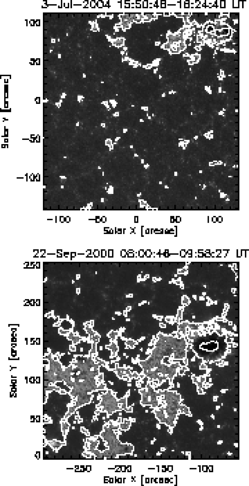
The chromospheric data studied were obtained by the Transition Region and Coronal Explorer (TRACE; Handy et al., 1999). Two $256\times 256$ arcsec² regions were recorded in the TRACE UV passbands with a sampling of 0.5 arcsec pixel^-1 on 2004 July 3 and 2000 September 22, with no compensation for solar rotation. Details of both data sets are given in Table 1 while Figure 1 depicts the time–averaged 1700 Å emissions. In set 1, images were obtained in the order 1600 Å, 1700 Å, and 1550 Å with a strict 4 s timing offset because of the TRACE filterwheel set up, resulting in an overall stable cadence of 16 s for each individual passband, while set 2 comprised of successive 1550 Å, 1600 Å, 1700 Å, and white–light images with an average cadence of 22.7 s.

Figure 1.— Time–averaged TRACE 1700 Å images for set 1 (upper) and set 2 (lower). Overlaid thin (thick) contours mark the mdi $|50|$ G ($|500|$ G) level.

Initially, data from each UV passband were dark subtracted and flat fielded. Portions of any images with corrupted data were replaced by the temporal mean of the preceding and following images, and JPEG compression effects were removed. Following DeForest (2004), data were derippled in both space and time by thresholding and removing spikes in the spatio–temporal Fourier domain. A final sweep of despiking was applied to remove cosmic ray hits and persistent “hot pixels” were removed from the data. After this processing, each UV passband datacube was co–aligned by spatially cross correlating every image to the mid–image of the respective time sequence. Although difficult to attribute heights of formation (HOF) to the broadband UV emissions (due to the large range of temperature coverage involved in their production, and the large HOF overlap between the 1700 Å and 1600 Å passbands), we assumed that the HOF increased from the 1700 Å passband to 1600 Å and then to 1550 Å (McAteer et al., 2004; Fossum & Carlsson, 2005b). Mid–images of the 1600 Å and 1550 Å data were separately co–aligned to the mid–image of the 1700 Å datacube for each data set, to achieve alignment between passbands. The 1700 Å data were taken as the reference for the alignment process because this passband has the response function with the lowest formation height in the solar atmosphere out of the TRACE passbands (formed around the temperature minimum; Judge et al., 2001), thus allowing for a better reference comparison for the alignment to the underlying magnetic field data.

Photospheric line–of–sight (LOS) magnetic field data were obtained by the Michelson Doppler Interferometer (mdi; Scherrer et al., 1995) on board the Solar Heliospheric Observatory (SoHO; Fleck et al., 1995). These data consist of longitudinal magnetic field measurements recorded with a spatial sampling of 0.6 arcsec pixel^-1, as mdi was operating in high–resolution mode. The mdi magnetograms were processed to Level–1.8 by the standard data pipeline and compensated for the roll angle of the SoHO spacecraft as well as the difference in image scales due to the differing observing positions of the satellites. In the case of set 2, magnetograms were co–aligned in the same manner as the UV datacubes before taking the temporal mean. Finally, mdi pixels corresponding to the time–rotated TRACE field–of–view (FOV) were re–sampled to the TRACE pixel size. The correlation of the co–spatial portions of the two data sets is shown by the contours in Figure 1. This form of mdi–to–TRACE alignment was verified by spatially cross correlating the magnetic field magnitude to the intensity of the TRACE 1700 Å mid–image, achieving sub–pixel accuracy.

Figure 2.— Upper: Frequency distribution of the total number of pixels (ordinate) in the selected mdi absolute field strength intervals (abscissa) for set 1. Lower: Percentages of the total number of pixels which show detections in each of the three TRACE UV passbands. The distributions for detections in the 1700 Å, 1600 Å, and 1550 Å data are shown in dotted, dashed, and dotted–dashed lines, respectively.

It is important that the field strengths presented here are, as for any magnetogram instrument, interpreted as the integration of net flux over a pixel area. Berger & Lites (2003) have shown, through direct comparison to the more reliable spectropolarimetry of the Advanced Stokes Polarimeter (asp), that mdi systematically underestimates the true longitudinal flux when operated in full–disk mode. However, we choose to report raw mdi values because our work makes use of mdi data obtained in high–resolution mode and the Berger & Lites correction factors may not be accurate — the difference in pixel sampling, and thus spatial flux averaging, should affect the slope of the mdi–asp flux–flux relation.

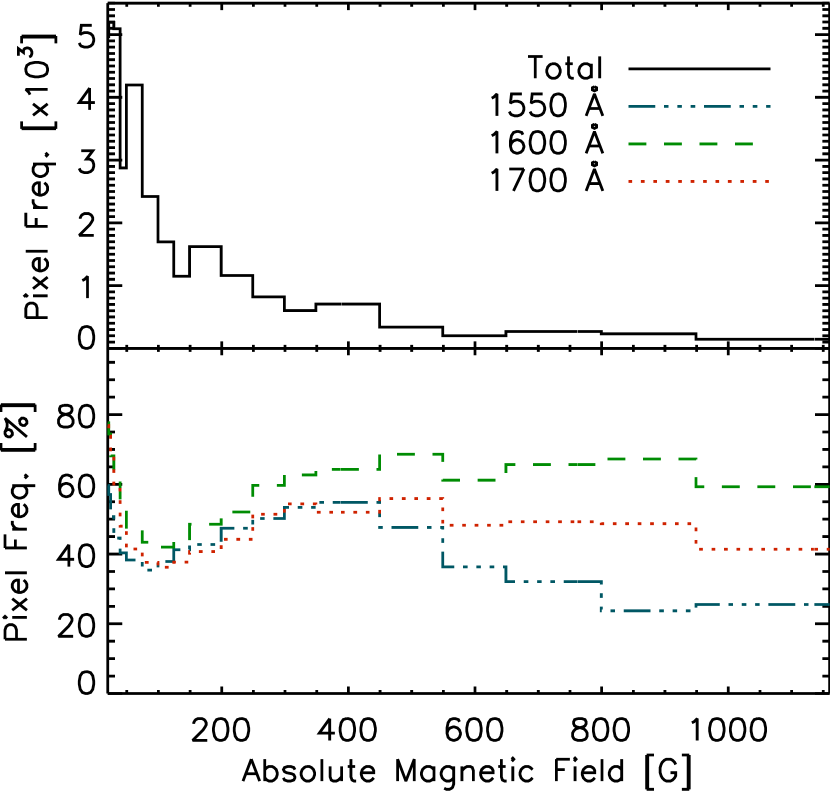
A magnetic field binning scheme was used in order to study oscillatory parameters in the TRACE UV data as a function of the absolute mdi magnetic field. Initially intervals of equal size were used, but the number of pixels decreases rapidly with increasing field strength. To counteract this, pixels with field strength values above $|20|$ G were instead separated into bins of systematically increasing size (listed in the first column of Table 2). The lower limit to the mdi magnetic field strength intervals is directly based on the instrumental noise level being reported as $\sim$$|20|$ G (Scherrer et al., 1995). The probability distribution function (PDF) of pixels used in our work is illustrated for the case of set 1 in the upper panel of Figure 2, while the lower panel depicts the percentage of pixels that contain wavelet oscillation detections.

3. ANALYSIS METHODS

3.1. Wavelet Power Transform

One of the most prevalent tools that has been recently used in observational studies of oscillatory behaviour is the technique of wavelet analysis (see the excellent introduction provided by Torrence & Compo 1998 and its application to solar data in, e.g., De Moortel et al. 2000, McAteer et al. 2004, and McIntosh & Smilie 2004). This multiscale analysis is better suited than Fourier analysis to both the spatial and temporal non–stationarity exhibited by oscillations in the solar atmosphere. For our study of oscillatory signals we chose the standard Morlet wavelet, a Gaussian–modulated sine wave which has an associated Fourier period, $P$, corresponding to $1.03s$, where $s$ is the wavelet scale. The wavelet transform is a convolution of the time series with the analyzing wavelet function whereby the complete wavelet transform is achieved by varying the wavelet scale, which controls both the period and temporal extent of the function, and scanning this through the time series. Regions exist at the beginning and end of the wavelet transform where spurious power may arise as a result of the finite extent of the time series. These regions are referred to as the cone of influence (COI), having a temporal extent equal to the $e$–folding time of the wavelet function. For the case of the Morlet wavelet it has the form, $t_{d}=\sqrt{2}s=\sqrt{2}P/1.03$. This time scale is effectively the response of the wavelet function to noise spikes and is used in our detection criteria by requiring that oscillations have a duration greater than $t_{d}$ outside the COI. This imposes a maximum period above which we can not accept detections, since we are dealing with finite time series of duration $D_{tot}$. At this maximum period it follows that $P_{max}=1.03D_{tot}/3\sqrt{2}$ — for set 1 $D_{tot}$ is 2032 s and $P_{max}$ is 493 s, while $D_{tot}$ is 7060 s and $P_{max}$ is 1714 s for set 2.

The form of automated wavelet analysis carried out on these data has previously been presented in McAteer et al. (2004), although some revisions have been carried out for our work. Firstly, no filtering was applied to data set 1 because the duration of observation presented here (34 min) is small compared to that of the TRACE spacecraft orbital period ($\sim$$90$ min). Therefore, long–period variations due to changes in Earth upper–atmospheric transmission are of small amplitude when compared to shorter periods of solar origin. Secondly, the more stringent statistical criterion of oscillations being at least 99% confident is employed rather than previous values of 95%. Finally, all power in the transform is retained, even that in the COI. Any detection having power above the 99% level for at least $t_{d}$ outside the COI has the entire duration recorded, including any portion which falls in the COI. This modification helps somewhat to circumvent previous limits on durations of detections. Not only does the upper limit to the possible number of cycles decrease with increasing oscillatory period (since analyzing finite duration time series), but removing the COI decreases this upper limit more drastically as the COI both increases with period and occurs at the start and end of the wavelet transform. After a complete analysis, carried out on the time series of each spatial pixel in all three TRACE passbands, the output comprises the duration in oscillatory cycles and the period of every detection.

3.2. Fourier Phase Differences

A Fourier phase difference analysis was used to further study possible propagation characteristics of waves between the co–spatial 1700 Å and 1600 Å time series. These passbands were chosen based on the proximity of their peak formation heights (Fossum & Carlsson, 2005b). This form of Fourier analysis is a technique which allows investigation of the difference in waveforms between two time series. Using the phase information contained within the complex Fourier transform, via the equations discussed in detail by Krijger et al. (2001), the difference in cyclic phase, $\Delta\phi$, can be determined for each Fourier frequency component, $\nu$, with the quality of the values represented by the phase coherence. The pairs of 1700 Å and 1600 Å time series in this study are extracted from the same ($x$, $y$) pixel location, but the signals remain separated in the direction normal to the solar surface. In this scenario, phase differences can be interpreted as delays caused by the finite propagation speed of waves traveling between the formation heights. The 1700 Å data were linearly interpolated to the 1600 Å (equally–separated) times to compensate for timing offsets that result from the TRACE UV data acquisition (§ 2). These offsets require removal as they produce drifts in phase difference spectra with frequency (Krijger et al., 2001).

Figure 3.— Fourier phase differences (ordinate) between 2420 pairs of TRACE 1700 Å and 1600 Å time series as a function of oscillatory frequency (abscissa). Larger symbols and darker shading depicts increased weighting significance (i.e., increased Fourier cross–power and coherence). The phase difference gradient ($M_{\Delta\phi}$; solid line) was calculated by weighted least–squares fitting of a first–order polynomial to all points in the range $2.0-5.4$ mHz, indicated by vertical dotted lines.

At those frequencies over which a wave has a real solution to its dispersion relation, and may thus propagate, phase difference spectra between emission signals formed at two separate heights are expected to have the form,

$$\Delta\phi\left(\nu\right)\approx\frac{\Delta h}{v_{ph}}\nu\ ,$$ (1)

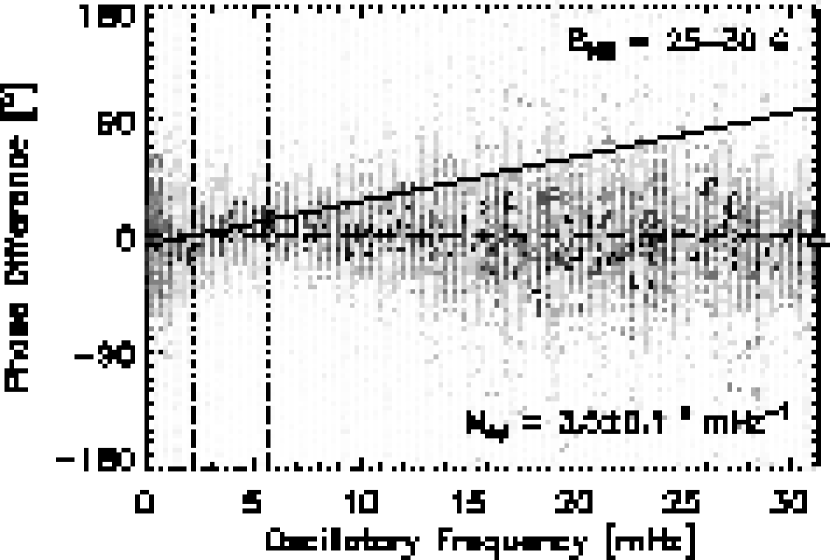
where $\Delta h$ is the separation distance of the emitting regions, $v_{ph}$ is the phase speed of the wave, and $\nu$ is the oscillation frequency. In a method similar to McIntosh et al. (2003), phase difference gradients ($M_{\Delta\phi}\approx\Delta h/v_{ph}$) were extracted over the frequency range $2.0-5.4$ mHz (periods $185-500$ s). This range was chosen because it encompasses the majority of our oscillation detections (§ 4.1). As shown in Figure 3, phase difference gradients were achieved by applying a weighted least–squares fit of a first–order polynomial to the phase difference spectra obtained from all time series originating from pixels in a particular range of field strengths. The contribution of each phase difference point to the fit was weighted by both the Fourier cross–power and coherence values.

4. RESULTS & DISCUSSION

Wavelet results are presented only for set 1 to avoid repetition, since set 2 displays similar behaviour with longer–period detections due to the increased duration of observation and more short–period detections from flare surges in the time series. However, Fourier results from both data sets are provided and discussed.

4.1. Wavelet Period Distributions

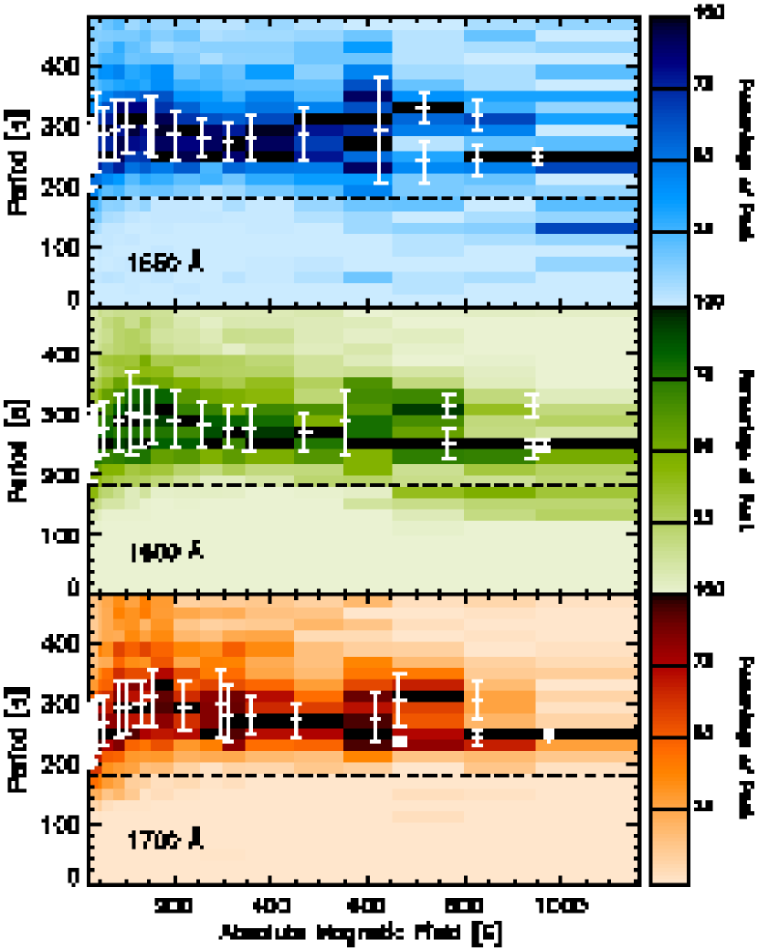
Detections in each mdi field strength interval were sampled in terms of their period with uniform $20$ s binning. The resulting 1700 Å, 1600 Å, and 1550 Å PDFs are shown in Figure 4, where the individual distributions are self–normalized to their peak number of detections to highlight changes between PDFs by compensating for the decreased number statistics at increased field strengths (Figure 2). Fitting profiles which consisted of a single Gaussian and a linearly increasing first–order polynomial (as most distributions showed a tail of detections at high periods) were applied to each PDF. Although the distributions are not ideally Gaussian, the variation of fitted centroid period ($P_{c}$; displayed as central bar marks in Figure 4 and detailed in Table 2) with mdi field strength and UV passband formation height should at least qualitatively describe these data. Bars extend over the $\pm$1$\sigma$ width of the Gaussian fit in Figure 4, representing PDF spread and not error in the fit. For each UV passband the symbols are plotted at the mean absolute field strength of the pixels which show oscillations in that passband. For a particular range of mdi field strengths the mean value will vary between each of the three UV passbands, a direct result of the differing pixel numbers which contribute to the different UV passband oscillation distributions (lower panel of Figure 2).

Figure 4.— Frequency distributions of TRACE 1700 Å (lower), 1600 Å (middle), and 1550 Å (upper) wavelet periods (ordinate) as a function of the mdi photospheric magnetic flux magnitude (abscissa). Distributions are normalized to their peak number of detections. Symbols mark centroid positions of Gaussian fits to each period distribution, with bars extending over the $\pm$1$\sigma$ width (detailed in Table 2). Points are overlaid at the mean mdi value of pixels showing detections in that field strength range. The dashed line marks the non–magnetic value of $P_{\mathrm{ac}}$ for $\theta=0$ at the temperature minimum.

Period PDFs in the range $|25-100|$ G shift to higher values of $P_{c}$ when moving to larger mdi field strengths. This progression of periods in the low chromosphere from 4– to 5– min agrees with the findings of Lawrence et al. (2003) who analyzed 3 Å–wide passband observations of Ca II K line intensity in the quiet–Sun (inter)network. Although the K₂ portion of the Ca II K line profile is formed at least somewhat above the temperature minimum (i.e., above these TRACE data), close agreement may still be expected with this work because the K₁ wing emission also contained in their broad passband is formed around the temperature minimum (Vernazza et al., 1981). Lawrence et al. attribute the period change to their passband being formed below the $\beta=1$ level at low field strengths and above it for higher fields, without offering a physical reason for the change. We draw attention to the fact that the periods detected are incompatible with standard MHD theory, where waves can only propagate at periods below the acoustic cutoff ($P_{\mathrm{ac}}\propto\sqrt{T}$; $T$ is temperature). As such, waves up to $\sim$5 min period can propagate into the photosphere (e.g., $p$ modes) but the temperature decrease with height in the low chromosphere acts to decrease the cutoff period and previously propagating long–period waves become evanescent.

We extend the hypothesis of Lawrence et al. (2003) by proposing that wave propagation may be permitted and the period behaviour explained using both the direct dependence that $P_{\mathrm{ac}}$ has on the magnetic field strength (Bel & Mein, 1971) and the inclination, $\theta$, which arises through the effective gravity, $g$ ($P_{\mathrm{ac}}\propto 1/g=1/g_{0}\cos\theta$, where $g_{0}=274$ m s^-1; De Pontieu et al., 2004). As shown by Lawrence et al. (2003), regions of increased magnetic field experience the $\beta=1$ level at lower altitudes. This intuitively suggests that the “magnetic canopy”, where the field spreads nearly horizontally, will be formed lower. If for low field strengths a HOF lies significantly below the “canopy” level it will experience near–vertical field lines. However, as the photospheric flux increases, the $\beta=1$ and “canopy” levels will be pulled down toward the HOF such that it samples increasingly inclined fields. The larger inclination acts to reduce the effective gravity, which in turn increases the cutoff period allowing for “tunneling” of evanescent wave modes (De Pontieu et al., 2004). Over the range $|22-75|$ G, increasing values of $P_{c}$ are recorded when moving upward through the UV passband HOFs, agreeing with this picture of sampling field lines of increasing inclination with height.

Table 2Magnetic Field Strength Intervals and Fit Parameters to Wavelet Period Distributions of 2004 July 03 (Set 1)

mdi Field	1700 Å Period		1600 Å Period		1550 Å Period
(G)	(s)		(s)		(s)
	$P_{c}$	1$\sigma$	$P_{c}$	1$\sigma$	$P_{c}$	1$\sigma$
$|20-22|$	238.3	$\pm 47.1$	236.6	$\pm 49.6$	242.7	$\pm 52.6$
$|22-25|$	238.6	$\pm 46.4$	239.0	$\pm 48.8$	244.0	$\pm 49.1$
$|25-30|$	243.9	$\pm 48.8$	245.2	$\pm 53.3$	250.2	$\pm 50.0$
$|30-40|$	253.8	$\pm 47.8$	257.6	$\pm 48.4$	266.7	$\pm 45.9$
$|40-50|$	261.2	$\pm 46.0$	268.3	$\pm 44.7$	288.6	$\pm 66.6$
$|50-75|$	270.0	$\pm 41.2$	276.6	$\pm 45.8$	284.8	$\pm 43.6$
$|75-100|$	289.9	$\pm 48.8$	288.5	$\pm 47.8$	293.6	$\pm 49.6$
$|100-125|$	293.6	$\pm 42.5$	302.7	$\pm 66.8$	300.4	$\pm 44.8$
$|125-150|$	298.3	$\pm 39.6$	296.7	$\pm 49.8$	300.9	$\pm 48.5$
$|150-200|$	310.0	$\pm 47.1$	298.4	$\pm 48.8$	297.6	$\pm 50.3$
$|200-250|$	294.0	$\pm 40.3$	290.1	$\pm 47.2$	283.5	$\pm 38.7$
$|250-300|$	298.5	$\pm 58.7$	282.1	$\pm 38.3$	279.3	$\pm 31.6$
$|300-350|$	282.9	$\pm 44.5$	278.7	$\pm 36.4$	275.3	$\pm 32.8$
$|350-450|$	279.9	$\pm 31.2$	278.1	$\pm 36.0$	279.8	$\pm 35.5$
$|450-550|$	270.7	$\pm 25.8$	270.3	$\pm 32.0$	286.2	$\pm 41.4$
$|550-650|$	273.9	$\pm 40.9$	287.1	$\pm 54.4$	293.0	$\pm 87.1$
$|650-800|$	236.4	$\pm 8.2$	252.0	$\pm 23.7$	239.6	$\pm 33.9$
$\cdots$	307.0	$\pm 43.9$	314.0	$\pm 18.3$	329.5	$\pm 25.0$
$|800-950|$	243.3	$\pm 12.8$	243.7	$\pm 16.0$	242.4	$\pm 25.9$
$\cdots$	305.4	$\pm 33.5$	311.9	$\pm 18.7$	316.1	$\pm 25.6$
$|950-1200|$	245.7	$\pm 6.1$	247.9	$\pm 9.9$	248.3	$\pm 13.2$
$>|1200|$	$\cdots$	$\cdots$	$\cdots$	$\cdots$	$\cdots$	$\cdots$

All three UV passbands subsequently show decreasing centroid periods when moving into regions of increased magnetic field ($|125-550|$ G). This differs from the results of Lawrence et al. (2003) where the peak wavelet power was observed at a fairly constant 5–min period for field strengths in the range $|200-500|$ G, although a marginal downturn in period may exist at their highest fields. However, it should be noted that the solar environment studied by Lawrence et al. (2003) contained neither plage nor sunspot regions which contribute to those field strengths in this work. A more appropriate comparison can be made with data set 2 previously presented in McIntosh & Smilie (2004) which is our set 2. Although not discussed, comparing the detected wavelet frequency in their Fig. 5 with the magnetic field shows the same variation: short period oscillations in the internetwork, increasing periods in areas of network and outer plage, and a decrease in period in those plage regions corresponding to the strongest plage magnetic fields.

The mdi intervals containing all but the largest field strengths ($|650-950|$ G) exhibit double–peaked PDFs. This makes qualitative sense as a sunspot lies in the FOV. As such, the lower–period components contain the $\sim$3–min umbral oscillations (Giovanelli, 1972, more distinct in data set 2 for fields $>|1200|$ G where periods peak at $160-180$ s), while components at higher periods contain the $\sim$5–min penumbral oscillations (Beckers & Schultz, 1972; Moore & Tang, 1975). It should be noted that period PDFs for all passbands do not appear double peaked at the highest fields ($>|950|$ G), despite showing decreased number statistics. The disappearance of a higher–period component at these largest field strengths supports their interpretation as penumbral oscillations since these fields should sample only umbral regions.

4.2. Wavelet Duration Distributions

An alternate way by which to characterize oscillations is their duration of observation, since this quantity can be interpreted as a measure of the energy associated with a wave. As such, detections were sampled in terms of their duration with uniform half–cycle binning. The resulting PDFs are shown separately in Figure 5 for the 1700 Å, 1600 Å, and 1550 Å data, where every PDF is again normalized to its peak number of detections. In these plots the most frequently detected duration is marked by a ‘$+$’ symbol, and differing dependencies on the magnetic field are clearly seen. The 1700 Å data have oscillations of duration $2.5-3$ cycles most frequently observed across the majority of magnetic fields, while the 1600 Å data also peak at $2.5-3$ cycles over most field strengths. The large degree of similarity between the behaviours of these two sets of distributions strongly implies that both UV passbands are formed in essentially the same physical environment. However, the 1550 Å durations peak at $1.5-2$ cycles over low field strengths ($|25-100|$ G) before changing to $2.5-3$ cycles for moderate magnetic fields ($|100-450|$ G). The oscillation durations then shorten to $2-2.5$ cycles for nearly all higher field strengths.

Figure 5.— As Fig. 4, but for TRACE 1700 Å (lower), 1600 Å (middle), and 1550 Å (upper) durations of wavelet detection (ordinate). Symbols mark the most frequently detected duration, plotted at the mean field strength of pixels showing oscillations in that field strength range.

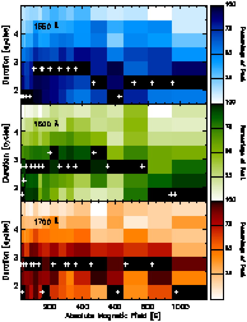
It appears that, if these oscillations are indeed waves, below $|100|$ G some portion of the wave energy budget has been lost between the formation heights of 1600 Å and 1550 Å, since the 1550 Å data exhibit durations shorter than both the 1700 Å and 1600 Å data. By contrast, the wavelet detection durations are conserved in the stronger–field range $|100-450|$ G which, in turn, indicates that the effective “boundary” previously lying between the 1600 Å and 1550 Å HOFs has been lowered in altitude to below the 1700 Å HOF. Incorporating a potential–field extrapolation, Lawrence et al. (2003) interpret their change from 4– to 5– min periods at field strengths of $\sim$$|150|$ G as resulting from the lowering of the $\beta$–unity surface below the formation height of their Ca II K line emission. This is very close to our wavelet duration transition field strength of $|100|$ G, while the disparity may be explained by the difference in passband formation heights and/or the assumption of the static, spatially–averaged VAL C model atmosphere (Vernazza et al., 1981) in the extrapolation.

4.3. Fourier Phase Speeds

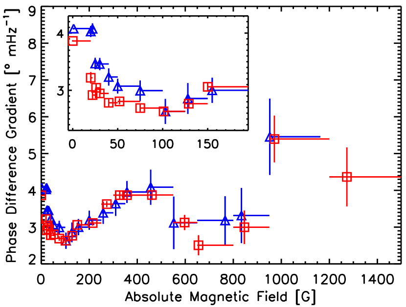
Although highly versatile and a powerful tool for studying oscillatory behaviour, the wavelet analysis performed up to now has not been able to distinguish whether the detected oscillations are the signatures of propagating waves in the solar atmosphere. It is for this reason that Fourier phase difference analysis was applied to the same data. The results of the analysis, outlined in § 3.2, are presented in Figure 6 for both data sets as the weighted–fit values of phase difference gradient between the 1700 Å and 1600 Å time series pairings.

Figure 6.— Fourier phase difference gradients ($M_{\Delta\phi}$; ordinate) between the 1700 Å and 1600 Å intensity time series as a function of mdi magnetic flux magnitude (abscissa) — triangles correspond to set 1 and squares to set 2. Symbols are plotted at the mean absolute field strength value, where horizontal bars denote the extent of the field strength range and vertical bars mark the $\pm$1$\sigma$ uncertainty to the weighted least–squares linear fits. The values obtained over low–field values are displayed within the inset to highlight fine detail.

If a spatially–invariant atmosphere is assumed, the vertical separation of UV HOFs will not vary when moving into regions of increased magnetic field. As a result, $\Delta h$ is constant and Equation 1 informs us that a change in Fourier phase difference gradient denotes the inverse of the change that has occurred in the wave phase speed. In the past, such forms of atmosphere have been used to implement potential–field extrapolations (e.g., McIntosh et al., 2003; Lawrence et al., 2003). Unfortunately, these act to oversimplify the complexity of the magnetic atmosphere and the application of 1–D models that take account of the differences between regions of differing magnetic field will yield more appropriate results.

From consideration of Equation 1, it is possible that the initial decrease of gradient values in Figure 6 could result from waves having the same phase speed but the HOF separations are reduced with increasing magnetic field. This suggests that $M_{\Delta\phi}$ should continue decreasing for even stronger fields, but we detect a switch in behaviour to increasing $M_{\Delta\phi}$ in the range $|125-550|$ G which requires increasing separations between the HOFs. This change in separation behaviour does not make qualitative sense, so we proceed by assuming a spatially–invariant atmosphere that yields increasing wave phase speeds up to $|100-125|$ G and a subsequent decrease in speeds up to $|550|$ G. A decrease in TRACE UV phase difference gradient with increasing magnetic field has been previously observed by McIntosh et al. (2003) with no turnaround reported. The deviation of our results can be explained by their quiet–Sun (inter)network data having fields $\leq$$|50|$ G so the $\beta=1$ level was not lowered below the UV HOFs, while wavelet durations imply that this occurs for fields $\geq$$|100|$ G in this study.

The observed wave speed behaviour over low– to moderate– magnetic fields may be interpreted as resulting from a change in physical environment within our pixel sampling rather than merely a variation of magnetic field. In regions spatially removed from the large flux concentrations of sunspots and plage, photospheric magnetic fields are believed to be unresolved kilo–Gauss elements, covering a small fraction of the pixel area (Lites, 2002; Domínguez Cerdeña & Kneer, 2003). In such cases the magnetic filling factor, $f$, is much less than unity and pixels will contain a contribution from both the ambient high–$\beta$ plasma and low–$\beta$ flux concentrations. In the high–$\beta$ material, magnetoacoustic slow modes have negligible density variations and are unobservable to our broad UV passbands, while the compressible fast modes will propagate between $c_{S}$ and $\sqrt{c_{S}^{2}+v_{A}^{2}}$ ($\approx c_{S}$ since $\beta\gg 1$). In the flux concentrations, slow–magnetoacoustic waves will propagate at $c_{S}$ (since $\beta<1$) while fast modes propagate between $v_{A}$ and $\sqrt{c_{S}^{2}+v_{A}^{2}}$. If these flux concentrations satisfy certain requirements they may be thought of as “thin flux tubes” (Roberts, 1985), in which slow modes propagate at the tube speed. Values of $0.2-0.5$ are typically used for plasma–$\beta$ in the modeling of flux tubes (e.g., Hasan et al., 2003, 2005), yielding tube speeds of $\sim$$0.9c_{S}$ and fast–mode speeds between $\sim$$(1.5-2.4)c_{S}$ and $\sim$$(1.8-2.6)c_{S}$. In this picture, the lowest field strengths arise from small values of $f$ so the measured speed is dominated by the “flux–external” sound speed, while for higher field strengths the filling factor increases and the contribution from the “flux–associated” speeds becomes more important.

Eventually, a filling factor of unity is reached and the passbands are formed in an homogeneously distributed magnetic environment for greater field strengths. The change from inhomogeneous to homogeneous environments ends the “flux tube” supported wave scenario. When $f=1$, the magnetic field has expanded to fill the entire pixel area, creating a “magnetic canopy” over the previously “flux–external” plasma. This marks the transition from mixed high– and low– $\beta$ to entirely low–$\beta$ environment (i.e., the $\beta=1$ level) and is signaled by the change in trend of phase difference gradient at fields of $|100-125|$ G. Although kilo–Gauss magnetic elements have been mentioned and field strengths of $|100-125|$ G are reported for filling factors of unity, field values are measured at the photosphere while $f$ corresponds to the region of the chromosphere where waves are detected and field lines have expanded into a greater spatial area.

Inside the subsequent homogeneous low–$\beta$ atmosphere, the fast–mode propagates at $v_{A}>c_{S}$, tending to $\gg$$c_{S}$ when $\beta\ll 1$. The initial fast–mode speed in the homogeneous situation (i.e., when $\beta=1$) is expected to be at most $\sim$$\sqrt{2}c_{S}$, yielding a phase difference gradient which differs from the field–free case by a factor of $\sim$$0.7$ (within the error bars of the ratio between our values recorded at $|100-125|$ G and $|0-20|$ G). The slow mode is again quasi–longitudinal and propagates at $c_{S}$. We note that the sound speed should not change between field strengths since it depends only on temperature ($\propto$$\sqrt{T}$) and the wave behaviours reported here occur between the same two UV passbands, which are formed over the same range of temperatures irrespective of magnetic field. The gradual decrease of wave speeds in the range $|125-550|$ G is taken as a signature of both modes existing within our signal, with the measured value of $M_{\Delta\phi}$ resulting from averaging between the two speeds. The increase of phase difference gradient with increasing magnetic field towards a similar value as detected over field strengths in the small filling factor range of $|0-20|$ G implies that the wave speeds are tending toward the sound speed, and slow–mode waves become dominant in our stronger field regions of plage and umbrae. An implication of slow–mode dominance in regions of stronger field is that slow modes propagate higher into the atmosphere than fast modes (Osterbrock, 1961) — the “magnetic canopy” occurs at lower altitudes when moving to higher field strengths, the UV passbands are formed progressively further above the $\beta$–unity level, and we detect only the speeds of modes which propagate higher into the atmosphere. The disclosure of these waves as slow modes provides a direct, and necessary, link to coronal studies (De Moortel et al., 2002), where propagating intensity variations at 3– and 5– min periods are interpreted as slow–magnetoacoustic waves in loops anchored in umbrae and plage, respectively. We note a disparity between the abundance of wave signatures in the low chromosphere and the sparse detection of slow–mode associated phenomena in the transition region (De Pontieu et al., 2004) and corona (De Moortel et al., 2002). Some mechanism is clearly required to quench most of these lower atmospheric waves with one possibility being slow–mode driven Pedersen current dissipation (Goodman, 2000), theorised to be highly efficient in the chromosphere. The non–uniformity observed in the upper atmosphere may highlight other selection effects at work on wave transmission, possibly based on $p$–mode interference with complex field orientations. Field inclinations affected by $p$–modes may also help explain the temporal intermittency of waves by only providing suitable propagation conditions over short, repeating timescales.

It should be noted that some penumbral pixels may be misinterpreted as weaker field regions from of the LOS nature of mdi and the existence of highly–inclined, outer–penumbral magnetic fields, e.g., field strengths of $|800-1000|$ G inclined 80° to the vertical (Solanki et al., 1992) will be recorded as $|140-175|$ G. However, pixels misclassified as such will not greatly modify the phase difference gradients, as the true weak–to–moderate field pixels ($|25-550|$ G) dominate the number statistics. Instead they contribute to greater error–bar magnitudes at higher field strengths, alongside the decrease in pixel numbers. Larger errors associated with gradient values above $|550|$ G may arise from averaging between the sunspot $\sim$3– and 5– min distributions, if propagating at different speeds. Decreased gradient values over $|550-950|$ G from those at fields both above and below complements this interpretation, as period PDFs exhibit widening toward and the detection of 5–min penumbral oscillations over this range. Hence, by causing decreased phase difference gradients, penumbral waves appear to either travel faster than those in umbrae and plage or experience a reduction in the HOF separations, distinctly possible for a penumbral atmosphere stratified along field lines at inclinations of $40-70$° (Mathew et al., 2003).

5. CONCLUSIONS

Chromospheric intensity variations have been studied using both time–localized wavelet and Fourier analysis. Investigation of the oscillation behaviours has identified three regimes with distinctly differing properties.

The increase of wavelet period with mdi field over $|25-100|$ G marks the modification of the magnetoacoustic cutoff period by field inclination effects. This arises from the “magnetic canopy” being pulled progressively closer to the sampled HOFs so that they experience more inclined fields. Wavelet durations show a decrease in the 1550 Å data over those in the 1600 Å and 1700 Å data, indicating a loss of wave energy. This can be explained by waves undergoing mode conversion or reflection at the $\beta$–unity surface (Bogdan et al., 2003). Fourier analysis indicates that wave phase speeds increase with magnetic field between the 1700 Å and 1600 Å formation heights. It is proposed here that this is due to an increase in magnetic filling factor within the pixel sampling, yielding a greater contribution to the observed wave speed from the low–$\beta$ “flux–associated” fast–mode speed over the slower sound speed of the surrounding high–$\beta$ plasma.

The similarity of wavelet periods and durations over field strengths in the range $|100-450|$ G implies that waves in this regime do not experience a drastic change in their environmental topology as evidenced by the weaker–field case. The $\beta$–unity surface is believed to lie below the formation height of 1700 Å emission, no transitional interface exists between the passbands, and wave energy (i.e., wavelet duration) is conserved with altitude. In contrast to the weak–field regime wave speeds decrease, which may be a signature of a change from dominant fast–mode magnetoacoustic waves to slow–mode waves when moving from network into plage.

Wavelet period distributions broaden and display a doubly–distributed nature over $|550-950|$ G, marking the sampling of sunspot regions. Interpretation of the 5–min component as being of penumbral origin is given strong support by the virtual disappearance of these higher–period components when sampling field strengths $\geq$$|950|$ G (i.e., umbrae). The decrease of phase difference gradient values over the mixed penumbral/umbral field strength range ($|550-950|$ G) suggests that either penumbral waves travel at greater speeds than those in plage and umbral regions or the formation heights of the 1700 Å and 1600 Å passbands are closer in altitude (e.g., because of inclined fields) in the penumbra.

In the future, we will be able to better determine the intricate relationship between magnetic topology and propagating waves using high–resolution, vector magnetic field information. Such data will soon be obtained by the full–Stokes spectropolarimeter in the instrument suite of the Solar Optical Telescope (sot) Focal Plane Package (fpp) on board Solar–B. Coordinated observations between this instrument, TRACE, and the multi–wavelength tunable filters also contained in the sot/fpp will yield diffraction–limited, high–cadence imaging at multiple heights through the outer Solar atmosphere unparalleled by previous observations. The combination of these forms of data with a range of atmospheric models taking into account the differences in atmospheric stratification for differing magnetic fields will yield a powerful diagnostic suite for studies of solar wave phenomena.

References

- Beckers & Schultz (1972) Beckers, J.M., & Schultz, R.B. 1972, Sol. Phys., 27, 61
- Bel & Mein (1971) Bel, N., & Mein, P. 1971, A&A, 11, 234
- Berger & Lites (2003) Berger, T.E., & Lites, B.W. 2003, Sol. Phys., 213, 229
- Bogdan et al. (2003) Bogdan, T.J., et al. 2003, ApJ, 599, 626
- Damé et al. (1984) Damé, L., Gouttebroze, P., & Malherbe, J.–M. 1984, A&A, 130, 331
- DeForest (2004) DeForest, C.E. 2004, ApJ, 617, L89
- De Moortel et al. (2000) De Moortel, I., Ireland, J., & Walsh, R.W. 2000, A&A, 355, L23
- De Moortel et al. (2002) De Moortel, I., Ireland, J., Hood, A.W., & Walsh, R.W. 2002, A&A, 387, L13
- De Pontieu et al. (2004) De Pontieu, B., Erdélyi, R., & James, S.P. 2004, Nature, 430, 536
- Deubner & Fleck (1990) Deubner, F.–L., & Fleck, B. 1990, A&A, 228, 506
- Domínguez Cerdeña & Kneer (2003) Domínguez Cerdeña, I., & Kneer, F. 2003, ApJ, 582, L55
- Domínguez Cerdeña et al. (2006) Domínguez Cerdeña, I., Sánchez Almeida, J., Kneer, F. 2006, ApJ, 636, 496
- Finsterle et al. (2004) Finsterle, W., Jefferies, S.M., Cacciani, A., Rapex, P., & McIntosh, S.W. 2004, ApJ, 613, L185
- Fleck et al. (1995) Fleck, B., Domingo, V., & Poland, A.I. eds. 1995, The SoHO Mission (Dordrecht: Kluwer)
- Fossum & Carlsson (2005a) Fossum, A., & Carlsson, M. 2005a, Nature, 435, 919
- Fossum & Carlsson (2005b) Fossum, A., & Carlsson, M. 2005b, ApJ, 625, 556
- Giovanelli (1972) Giovanelli, R.G. 1972, Sol. Phys., 27, 71
- Goodman (2000) Goodman, M.L. 2000, ApJ, 533, 501
- Handy et al. (1999) Handy, B.N., et al. 1999, Sol. Phys., 187, 229
- Hasan et al. (2003) Hasan, S.S., Kalkofen, W., van Ballegooijen, A.A., & Ulmschneider, P. 2003, ApJ, 585, 1138
- Hasan et al. (2005) Hasan, S.S., van Ballegooijen, A.A., Kalkofen, W., & Steiner, O. 2005, ApJ, 631, 1270
- Judge et al. (2001) Judge, P.G., Tarbell, T.D., & Wilhelm, K. 2001, ApJ, 554, 424
- Krijger et al. (2001) Krijger, J.M., Rutten, R.J., Lites, B.W., Straus, Th., Shine, R.A., & Tarbell, T.D. 2001, A&A, 379, 1052
- Lawrence et al. (2003) Lawrence, J.K., Cadavid, A.C., Miccolis, D., Berger, T.E., & Ruzmaikin, A. 2003, ApJ, 597, 1178
- Leighton et al. (1962) Leighton, R.B., Noyes, R.W., & Simon, G.W. 1962, ApJ, 135, 474
- Lites (2002) Lites, B.W. 2002, ApJ, 573, 444
- Lites et al. (1993) Lites, B.W., Rutten, R.J., & Kalkofen, W. 1993, ApJ, 414, 345
- Mathew et al. (2003) Mathew, S.K., et al. 2003, A&A, 410, 695
- McAteer et al. (2004) McAteer, R.T.J., Gallagher, P.T., Bloomfield, D.S., Williams, D.R., Mathioudakis, M., & Keenan, F.P. 2004, ApJ, 602, 436
- McIntosh et al. (2003) McIntosh, S.W., Fleck, B., & Judge, P.G. 2003, A&A, 405, 769
- McIntosh & Smilie (2004) McIntosh, S.W., & Smilie, D.G. 2004, ApJ, 604, 924
- Moore & Tang (1975) Moore, R.L., & Tang, F. 1975, Sol. Phys., 41, 81
- Osterbrock (1961) Osterbrock, D.E. 1961, ApJ, 134, 347
- Roberts (1985) Roberts, B. 1985, in Solar System Magnetic Fields, ed. Priest, E.R. (Dordrecht: Reidel), 37
- Rosenthal et al. (2002) Rosenthal, C.S., et al. 2002, ApJ, 564, 508
- Scherrer et al. (1995) Scherrer, P.H., et al. 1995, Sol. Phys., 162, 129
- Socas–Navarro (2005) Socas–Navarro, H. 2005, ApJ, 633, L57
- Solanki et al. (1992) Solanki, S.K., Rueedi, I., Livingston, W. 1992, A&A, 263, 339
- Torrence & Compo (1998) Torrence, C., & Compo, G.P. 1998, Bull. Am. Meteor. Soc., 79, 61
- Vernazza et al. (1981) Vernazza, J.E., Avrett, E.H., & Loeser, R. 1981, ApJS, 45, 635