THE MARENOSTRUM UNIVERSE

The MareNostrum Universe is one of the biggest SPH cosmological simulations done so far. It contains more than 2 billion particles ($2\times 1024^{3}$) in a 500 h^-1 Mpc cubic volume. This simulation has been performed on the MareNostrum supercomputer at the Barcelona Supercomputer Center. We have obtained more than 0.5 million halos with masses greater than a typical Milky Way galaxy halo. We report results about the halo mass function, the shapes of dark matter and gas distributions in halos, the baryonic fraction in galaxy clusters and groups, baryon oscillations in the dark matter and the halo power spectra as well as the distribution and evolution of the gas fraction at large scales.

1 Numerical Simulation and Data Analysis

In our numerical simulation we have assumed the spatially flat concordance cosmological model with the parameters $\Omega_{m}=0.3$, $\Omega_{bar}=0.045$, $\Omega_{\Lambda}=0.7$, the normalization $\sigma_{8}=0.9$ and the slope $n=1$ of the power spectrum. Within a box of $500{{h^{-1}{\rm Mpc}}}$ size the linear power spectrum at redshift $z=40$ has been represented by $1024^{3}$ DM particles of mass $m_{\rm DM}=8.3\times 10^{9}h^{-1}{{{\rm{M_{\odot}}}}}$ and $1024^{3}$ gas particles of mass $m_{\rm gas}=1.5\times 10^{9}h^{-1}{{{\rm{M_{\odot}}}}}$. The nonlinear evolution of structures has been followed by the GADGET II code of V. Springel $\!{}^{{\bf?}}$. For the gravitational evolution we have used the TREEPM algorithm on a homogeneous Eulerian grid to compute large scale forces by the Particle-Mesh algorithm. In this simulation we employed $1024^{3}$ mesh points to compute the density field from particle positions and FFT to derive gravitational forces. Since the baryonic component is also discretized by the gas particles all hydrodynamical quantities have to be determined using interpolation from the gas particles. Within GADGET the equations of gas dynamics are solved by means of the Smoothed Particle Hydrodynamics method in its entropy conservation scheme. To follow structure formation until redshift $z=0$ we have restricted ourselves to the gas-dynamics without including dissipative or radiative processes or star formation. The spatial force resolution was set to an equivalent Plummer gravitational softening of $15\;h^{-1}$ comoving kpc. The SPH smoothing length was set to the distance to the 40^th nearest neighbor of each SPH particle. In any case, we do not allow smoothing scales to be smaller than the gravitational softening of the gas particles. Using for three weeks 512 processors of the MareNostrum supercomputer at BSC Barcelona (this time corresponds to 29 CPU years) we have finished the simulation and created the MareNostrum Universe.

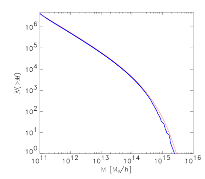
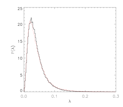
Figure 1: Left: Mass function of objects in the MareNostrum Universe, dotted line for Sheth-Tormen approximation. Right: Probability distribution of spin parameter of halos with more than 500 particles for virial overdensity (solid) and 8 times viral overdensity (dotted).

With 2 billion particles (DM and gas) the code produces 64 Gb of data per time step. To follow the evolution of structures we have stored 135 time steps equally separated by $10^{8}$ years. It is a challenge to find structures and substructures in the distribution of DM and gas particles. We have used a parallel hierarchical friends-of-friends algorithm which is based on the calculation of the minimum spanning tree of the given particle distribution. The minimum spanning tree of any point distribution is a unique, well defined quantity which describes the clustering properties of the point process completely. Based on the minimum spanning tree we sort the particles in such a way that we get a particle-cluster ordered sequence. Any object defined at any linking length is a segment of this sequence. Thus we can easily extract all objects and their substructures. The minimum spanning tree and the FOF-analysis have been done on JUMP Jülich.

In the left panel of Fig. 1 we show the total number of objects identified in the simulation with masses ($>M$). The MareNostrum Universe contains 4060 clusters of galaxies with masses larger than $10^{14}{{h^{-1}{\rm{M_{\odot}}}}}$, more than 58000 groups and clusters with masses larger than $10^{13}{{h^{-1}{\rm{M_{\odot}}}}}$. It contains about 0.5 million objects with masses between $10^{12}{{h^{-1}{\rm{M_{\odot}}}}}$ and $10^{13}{{h^{-1}{\rm{M_{\odot}}}}}$. In total we have identified at redshift $z=0$ more than 2 million objects with more than 20 DM particles. The spin parameter probability function is shown in Fig. 1 (right) for halos defined at different overdensities. The most likely value is $\lambda_{0}=0.023$, in good agreement with other numerical studies. There is no significant difference between the probability distribution of the spin parameters at virial and 8 times virial overdensity.

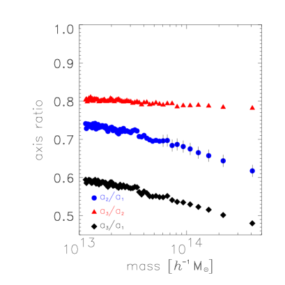
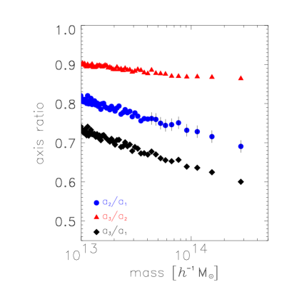
Figure 2: Left: The ratio between the main axes of the DM halos of clusters and groups depending on their mass. Right: The same for the gas distribution.

The shape of the objects can be described by three-axial ellipsoids with main axes $a_{1}\geq a_{2}\geq a_{3}$. In Fig. 2 we show the shape of group and cluster sized objects depending on mass. Filled circles denote the mean ratio of $a_{2}/a_{1}$ of 1000 objects in each bin. (The bars on the 10 most massive objects denote the corresponding Poisson errors; per definition they are identical in all bins.) On the left hand side we show the shape of the DM component and on the right hand side the shape of the gas component. The mass denotes always the total mass (DM + gas) of the object. Filled triangles denote the mean ratio of $a_{3}/a_{2}$ and filled diamonds $a_{3}/a_{1}$, the latter is roughly the product of the two previous. One can clearly see that the gas distribution is much more spherical than the DM distribution. In both cases more massive objects are more ellipsoidal. These objects have been formed later. With time they will become more spherical too.

Figure 3: Baryon fraction in clusters of galaxies.

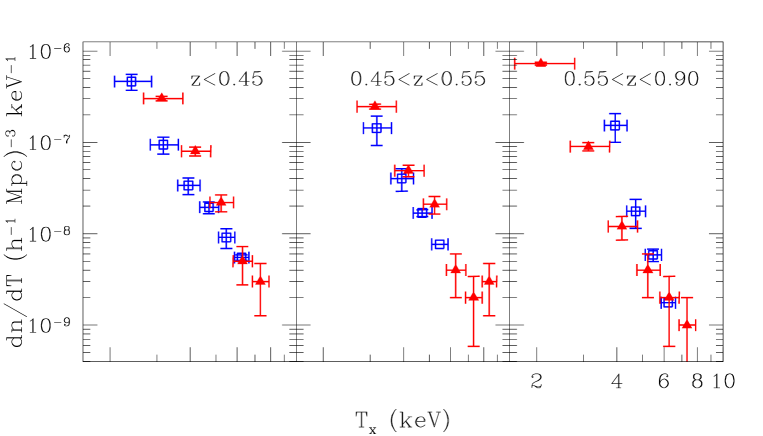
Figure 4: X-ray temperature function for simulated (filled triangles) and observed (open squares) CHANDRA clusters (Vikhlinin 2006) at different redshifts

2 Clusters of Galaxies

One of the aims of the simulation was to compare the large scale distribution of gas and DM. Since the shape of the gas distribution and the dark matter distribution in galaxy clusters is quite different we have determined the gas fraction in clusters within spheres centered at the highest density peak of the cluster. The highest density peak has been determined within the hierarchical friends-of-friends algorithm using a linking length which corresponds to 512 times the virial overdensity. The center of mass of this central object has been assumed to be the center of the cluster.

In Fig. 3 we show the baryon fraction in 4000 clusters with virial masses larger than $10^{14}{{h^{-1}{\rm{M_{\odot}}}}}$. The solid line denotes the cosmological baryon fraction of 0.15. One can clearly see that the baryon fraction in almost all of the clusters is below the cosmological one, the mean is about 0.14.

We have estimated the X-ray properties of the clusters found in this simulation. We used Sutherland & Dopita $\!{}^{{\bf?}}$ cooling curves for primordial composition to derive X-ray emission from gas particles. In Fig. 4 we compare the cluster abundance as a function of X-ray emission weighted temperature from the MareNostrum Universe with the most recent estimates from a sample of CHANDRA clusters $\!{}^{{\bf?}}$ up to $z\sim 1$. The agreement is remarkable at lower $z$, while we find a smaller number of clusters at high $z$ possibly due to resolution effects. Evolution of scaling relations have also been studied for our cluster sample. No significant evolution with redshift for the slope (range from 1.8 -2.1) of the $L_{x}-T_{x}$ is found.

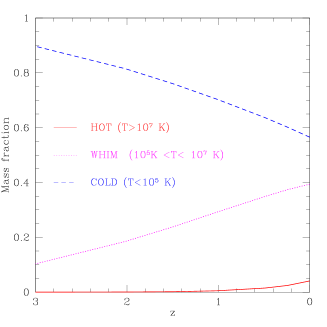
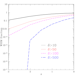
Figure 5: Left: Redshift evolution of the different baryon phases. Right: Evolution of WHIM at different overdensities.

3 Evolution of the Baryon Distribution at Large Scales

The large number of gas particles of this simulation allows us to compute accurately the redshift evolution of the baryonic phase space $(T-\rho_{gas})$. In Fig 5 we show the evolution of the relative fractions of the different baryon components: HOT, COLD and WARM-HOT gas. At present, the amount of gas in the form of WHIM is of the order of 40%. In the right panel of the same figure, we plot the evolution of the WHIM component above different comoving overdensities. The relative fraction increases rapidly at early redshift and becomes stable when the universe is dominated by exponential expansion ($z<0.5$ ). This is in good agreement with the assumption that baryons follow a lognormal density probability function $\!{}^{{\bf?}}$. At $\delta>50$ the WHIM are within virialized objects. We see that this amounts to 60% of the total WHIM at present. Therefore, we deduce that almost 40 % of baryons live in the WHIM phase in regions below viral overdensites, i.e. filaments and voids.

4 Baryonic Oscillations

The acoustic oscillations of the primordial plasma before recombination are not only reflected in the prominent peak structure of the CMB power spectrum but also imprinted in the power spectrum of the dark matter distribution, though the effect is much smaller ($\sim 5\%$) than for the CMB photons. The physical scale of these tiny wiggles is determined by the matter and baryon densities, which will be measured with high accuracy by the upcoming Planck mission. Knowing the physical size the baryonic wiggles then provide a standard ruler. If one is able to measure accurately enough the observed size of this standard ruler transverse and parallel to the line of sight at different redshifts, one is able to determine the angular diameter distance $D_{A}(z)$ and the Hubble parameter $H(z)$ for different redshifts and by this can constrain the equation of state parameter $w$ of the dark energy. For details see e.g. Seo & Eisenstein $\!{}^{{\bf?}}$.

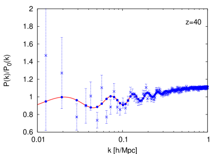
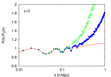
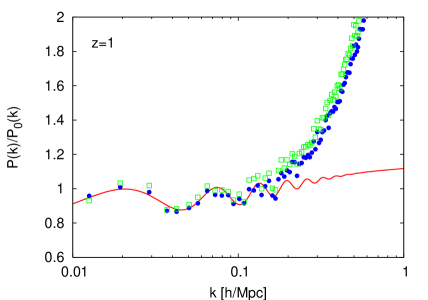
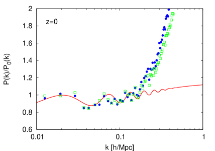
Figure 6: Real-space power spectra of the dark matter (filled circles) and of the halo (open squares) distributions at different redshifts. In all plots a linearly evolved power spectrum without baryons is divided out to make the baryonic oscillations more pronounced. At the upper left the actual realization of the initial power spectrum at redshift 40 is presented (crosses with error bars). The deviations from the mean power spectrum (solid line) due to the finite number of modes are corrected in all the other plots. In addition the halo power spectra are divided by $b^{2}$, where the bias factor $b$ is $2.78$ at $z=3$, 1.28 at $z=1$ and 0.94 at $z=0$.

With this simulation we were able to study qualitatively how the non-linear evolution and the effect of galaxy bias distort the baryonic oscillations. In Fig. 6 we show the real-space power spectra of the dark matter and FOF-cluster distribution. To enhance the visibility of the oscillations all power spectra have been divided by a linearly evolved power spectrum with the same cosmological parameters except for the baryon density being zero. To this end we used the fitting formula provided by Eisenstein & Hu $\!{}^{{\bf?}}$. In the upper left panel of Fig. 6 the realization (crosses) of the initial power spectrum (solid line) used to set up the initial conditions for the simulation at redshift 40 is shown. The deviations from the desired input power spectrum are due to the few modes available for the largest scales of the simulation box. These deviations make it impossible to detect the first peaks in a survey with a volume comparable to that of this simulation. To study nevertheless the effects of non-linear evolution and galaxy bias on the baryonic oscillation we correct all power spectra by these initial deviations.

At $z=3$ the first three peaks ($k\sim 0.7$, $k\sim 1.3$ and $k\sim 2.0\,h/{\rm Mpc}$) of the baryonic oscillations are clearly visible in the dark matter power spectrum. In the cluster power spectrum only the first two remain undistorted. For lower redshifts the non-linear evolution erases more and more the oscillation features. At $z=0$ one can hardly see any oscillation feature. Even the first peak is strongly distorted although it still does not lie in the non-linear regime.

We conclude that at high redshift ($z\sim 3$) the baryonic oscillation are conserved well enough even in the galaxy distribution to measure their scale accurately enough to constrain the equation of state parameter $w$ of the dark energy. The main problem will be to observe a high number of galaxies in a very large volume to reduce both cosmic variance and shot noise. For low redshifts it will be hard to measure the sound horizon with the required accuracy unless one understands the non-linear evolution well enough to reconstruct the baryonic oscillation. One tool to learn more about this are cosmological simulations.

References

References

- [1] V. Springel, MNRAS 364, 1105 (2005).
- [2] R.S. Sutherland and M.A. Dopita, ApJS 88, 253 (1993)
- [3] A. Vikhlinin, Proceedings of the XLIst Rencontres de Moriond ”From Dark Halos to Light” ed. L. Tresse, S. Maurogordato, J. Tran Than Van (2006)
- [4] F. Atrio and J. Mücket, ApJ 643, 1 (2006)
- [5] H.-J. Seo and D.J. Eisenstein, ApJ 598, 420 (2003)
- [6] D. J. Eisenstein and W. Hu, ApJ 496, 605 (1998)