On the extrasolar multi-planet system around HD 160691

Abstract

We re-analyze the precision radial velocity (RV) observations of HD160691 ($\mu$ Ara) by the Anglo-Australian Planet Search Team. The star is supposed to host two Jovian companions (HD160691b, HD160691c) in long-period orbits ($\sim 630$ days and $\sim 2500$ days, respectively) and a hot-Neptune (HD160691d) in $\sim 9$ days orbit. We perform a global search for the best fits in the orbital parameters space with a hybrid code employing the genetic algorithm and simplex method. The stability of Keplerian fits is verified with the $N$-body model of the RV signal that takes into account the dynamical constraints (so called GAMP method). Our analysis reveals a signature of the fourth, yet unconfirmed, Jupiter-like planet HD160691e in $\sim 307$ days orbit. Overall, the global architecture of four-planet configuration recalls the Solar system. All companions of $\mu$ Ara move in quasi-circular orbits. The orbits of two inner Jovian planets are close to the 2:1 mean motion resonance. The alternative three-planet system involves two Jovian planets in eccentric orbits ($e\sim 0.3$), close to the 4:1 MMR, but it yields a significantly worse fit to the data. We also verify a hypothesis of the 1:1 MMR in the subsystem of two inner Jovian planets in the four-planet model.

1. Introduction

The star HD160691 ($\mu$ Ara) is a Sun-like main-sequence dwarf monitored by the long-term, precision radial velocity (RV) surveys. It has been observed over more than 7 years by the Anglo-Australian Telescope (AAT) Planet Search Team and by the Geneva Planet Search Team (CORALIE and HARPS spectrometers). The work of the AAT team lead to the discovery of a Jupiter like companion HD160691b in about 630 days orbit (Butler et al., 2001). One year later, Jones et al. (2002) confirmed the Jovian planet and discovered a linear trend in the RV data revealing a signature of the second, more distant body. In the next paper, McCarthy et al. (2004) published a new orbital solution with the orbital period of the long-period planet HD160691c about 3000 days and the eccentricity $e_{{\mbox{\scriptsize c}}}\sim 0.57$. The same year, Santos et al. (2004), using observations done with the ultra precise HARPS spectrometer, announced $\sim 14$ Earth-mass planet HD160691d in $\sim 9$ days orbit. That discovery is a breakthrough in the field as the long-term precision of spectrometers approaches $1$ m/s. Actually, the instrumental errors are much smaller than the RV variability (stellar jitter) induced by the Sun-like stars themselves. Recently, Butler et al. (2006) published a new updated set of 108 observations of $\mu$ Ara, spanning 2551 days (about 7.5 yr). Thanks to the updates in the UCLES instrument installed at the AAT and the software pipeline (Butler et al., 2006), the long-term precision of the measurements is amazing. It also reaches $1$ m/s at the end of the observational window and is kept at the mean level of $\sim 2.8$ m/s over its whole length.

This paper is devoted to the analysis of the RV observations of $\mu$ Ara using the so called GAMP approach (an acronym of genetic algorithm with MEGNO penalty) that makes explicit the use of Newtonian, self-consistent $N$-body model of the stars’ reflex motion, dynamical properties of the planetary system and the Copernican Principle (Goździewski et al., 2003, 2005). This algorithm makes it possible to derive meaningful bounds on the elements of the outermost planet in spite of the fact that the data cover only a part of the longest orbital period. Without the dynamical constrains, the kinematical as well as pure Newtonian best fits to the $\mu$ Ara RV tend to show large eccentricity of the outermost companion and then the system becomes catastrophically unstable.

We verify the results of the previous papers based on a much smaller number of relatively less accurate RV observations. The results of the analysis of the new RV data set greatly improved and extended over time by Butler et al. (2006) lead us to a conclusion that the $\mu$ Ara may host four planets in quasi-circular orbits, including a new, Jupiter-like object in $\sim 307$ days orbit (HD160691e). The new best fit solution describes the orbital architecture of this extrasolar system as very different from the previous ones.

Shortly after submitting the manuscript, we learned about an independent work by Pepe et al. (2006) who announced a very similar orbital solution and also the fourth planet in the $\mu$ Ara system. These authors study a different set of the RV measurements but the conclusions of the two papers are in an excellent agreement. Still, in this paper we focus our attention on the analysis of the AAT data along the lines of the originally submitted manuscript. However, the last Section 5 is devoted to a preliminary study of the full available data set, including the new measurements published by Pepe et al. (2006). In particular, we verify a hypothesis of the 1:1 MMR in the subsystem of two Jovian planets.

2. Fitting multi-planet configurations to RV data

According to the previous papers devoted to $\mu$ Ara, the time range of the updated data set published by Butler et al. (2006) should be already close to the orbital period of the outermost companion. In that case, we can try to recover a good approximation of the system parameters by modeling the RV signal with the Keplerian orbits. Although for mutually interacting systems the kinematic model often leads to unstable orbital configurations, thanks to the numerical simplicity it can be very helpful to rapidly determine putative solutions and interesting ranges of orbital parameters.

The contribution of every planet to the reflex motion of the parent star at time $t$ is the following Smart (1949):

$$V_{{\mbox{\scriptsize r}}}(t)=K[\cos(\omega+\nu(t))+e\cos\omega]+V_{0},$$ (1)

where $K$ is the semi-amplitude, $\omega$ the argument of pericenter, $\nu(t)$ the true anomaly involving implicit dependence on the orbital period $P$ and the time of periastron passage $T_{{\mbox{\scriptsize p}}}$, $e$ the eccentricity, and $V_{0}$ is the velocity offset. Some argue that it is best to interpret the derived fit parameters $(K,P,e,\omega,T_{{\mbox{\scriptsize p}}})$ in terms of Keplerian elements and minimal masses related to Jacobi coordinates (Lee & Peale, 2003; Goździewski et al., 2003). We follow their reasoning when calculating the orbital elements from the primary fit parameters.

The extensive exploration of the multi-parameter ${(\chi^{2}_{\nu})^{1/2}}$ space is efficient enough if one applies a kind of a hybrid optimization (Goździewski & Konacki, 2004; Goździewski & Migaszewski, 2006). The idea of this algorithm relies on two steps, global and local ones. In the first step, we search for potentially good (but not very accurate) solutions in a global manner. During the second step these solutions become initial conditions to a precise and fast local algorithm. The single program run starts the genetic algorithm (GAs). In particular, we apply the PIKAIA code by Charbonneau (1995). The GAs have important advantages over more popular gradient-type methods (Press et al., 1992). The power of GAs lies in their basically global nature, the requirement of knowing only the ${(\chi^{2}_{\nu})^{1/2}}$ function, and the ease of constrained optimization; GAs permit defining parameter bounds according to specific requirements, or adding a penalty term to ${(\chi^{2}_{\nu})^{1/2}}$ (Goździewski et al., 2006). However, the best fits found with GAs are (in principle) not very accurate in terms of ${(\chi^{2}_{\nu})^{1/2}}$ or rms, so we refine them with another non-gradient algorithm, the simplex method of Melder and Nead (Press et al., 1992). Usually, we run such hybrid procedure thousands of times, and then we analyse the ensemble of gathered fits. That helps us to detect local minima of ${(\chi^{2}_{\nu})^{1/2}}$ that are sometimes very distant in the parameter space and to get reliable approximation of the global topology of ${(\chi^{2}_{\nu})^{1/2}}$. We tested the code extensively (Goździewski & Migaszewski, 2006), and we found many examples confirming its robustness and reliability. Remarkably, the code works with minimal requirements for user-supplied information: basically, one should only define the model function [so called fitness function, usually equal to $1/{(\chi^{2}_{\nu})^{1/2}}$] — conveniently, it is the same for the GAs and simplex, and to determine (even very roughly) parameter bounds for the assumed number of planets. We underline that the code is FFT-free, and by its construction, it works without any a-priori determination of the orbital periods.

In some cases (like strongly resonant or interacting systems, noisy data, a small number of measurements) the kinematic fits may lead to unrealistic, rapidly disrupting configurations. Then a more elaborate $N$-body Newtonian model of the RV should be applied (Rivera & Lissauer, 2001; Laughlin & Chambers, 2001). Yet the hybrid optimization can be still used as a general approach of exploring the parameter space (only the model function is changed). Actually, even more general modeling of the RV data relies on the elimination of the unstable (strongly chaotic) solutions during the fit process. That self-consistent approach follows the Copernican Principle and the complex structure of the phase space predicted by the Kolmogorov-Arnold-Moser theorem (Arnold, 1978). The idea of the dynamical fits with stability constraints relies on modifying the ${(\chi^{2}_{\nu})^{1/2}}$ function by a penalty term employing an efficient fast indicator MEGNO (Cincotta & Simó, 2000). We describe that method (GAMP) in detail in our past works (Goździewski et al., 2005, 2006).

To obtain reliable estimates of the fitted parameter errors, the internal measurement errors should be rescaled (Butler et al., 2004) according to $\sigma^{2}=\sigma_{{\mbox{\scriptsize m}}}^{2}+\sigma_{{\mbox{\scriptsize j}}}^{2},$ where $\sigma_{{\mbox{\scriptsize m}}}$ and $\sigma_{{\mbox{\scriptsize j}}}$ is the internal error and adopted dispersion of stellar jitter, respectively, and $\sigma$ is the joint uncertainty. Typically, we choose $\sigma_{{\mbox{\scriptsize j}}}$ following the estimates for Sun-like dwarfs by Wright (2005), or we use the value adopted by the discovery teams. The jitter estimate for $\mu$ Ara by Butler et al. (2006) is 3.5 m/s and we use this value in our calculations. The analysis of the short time-scale RV variability of the parent star may be found in Bouchy et al. (2005). The physical properties of the parent star are discussed in McCarthy et al. (2004) and Santos et al. (2004).

3. Three-planet model of the RV

In (Goździewski et al., 2003, 2005) we carried out an extensive analysis of the RV measurements published by Jones et al. (2002) and McCarthy et al. (2004) assuming that there exist two Jupiter companions of $\mu$ Ara. By employing the dynamical $N$-body model and GAMP, we obtained meaningful limits on the barely constrained orbital parameters of the putative outermost planet. According to our results, $a_{{\mbox{\scriptsize c}}}$ should be roughly greater that $4$ AU and $e_{{\mbox{\scriptsize c}}}<0.4$ in the range of the smallest permissible semi-major axes. The new precision RV data published by Butler et al. (2006) give us an excellent opportunity to verify these conclusions.

Figure 1 shows the results of the hybrid search for the putative three-planet configurations, in terms of multi-planet Keplerian model, assuming that the innermost planet has $P_{{\mbox{\scriptsize d}}}\in[7,12]$ days and $e_{{\mbox{\scriptsize d}}}\in[0,0.3]$, and that two Jupiter-like planets are in orbits with $P_{{\mbox{\scriptsize b}}}\in[100,1200]$ days, $P_{{\mbox{\scriptsize c}}}\in[1200,8500]$ days, and $e_{{\mbox{\scriptsize b,c}}}\in[0.0,0.8]$, respectively. These safe assumptions are consistent with the results of a few papers devoted to $\mu$ Ara. In particular, we rely on the careful analysis by Santos et al. (2004) and Bouchy et al. (2005) that revealed the hot-Neptune HD160691d. We might expect that its signal $K_{{\mbox{\scriptsize d}}}\sim 4$ m/s is comparable to the error level of the AAT data, nevertheless we decide to add this planet to the model, not to avoid the a-priori information on the system architecture. It appears that the hot-Neptune signal improves the rms by $\sim 0.5$ m/s, so it could be important to obtain a precise solution for the whole system.

The best fits obtained in the search are illustrated by projections onto the planes of particular parameters of the RV model, Eq. 1. Here, we choose the $(P,K)$- and $(P,e)$-planes. Marking the elements within the formal $1\sigma,2\sigma,3\sigma$ confidence intervals of the best-fit solution (signed by two crossing lines), we have a convenient way of visualizing the shape of the local minima of ${(\chi^{2}_{\nu})^{1/2}}$ and obtaining realistic and reasonable estimates of the parameter errors (Bevington & Robinson, 2003). Figure 1 illustrates the parameters of $\sim 1000$ different fits within the $3\sigma$ confidence interval of the best Fit I (its parameters are given in Table 1). Remarkably, the orbital period $P_{d}\sim 9.637$ days and the semi-amplitude $K_{d}\sim 3$ m/s are very close to the independent estimates by Santos et al. (2004), on the basis of HARPS measurements. Thus in spite of the RV contribution of the hot-Neptune planet d (of the inferred $\sim 11$ Earth-masses) being on the noise level $\sim 4$ m/s, the planet is already “visible” also in the AAT measurements. The two-planet Keplerian model of the RV yields ${(\chi^{2}_{\nu})^{1/2}}\sim 1.11$ and an rms $\sim 4.45$ m/s, so the signal of HD160691d improves the fit by $\sim 0.5$ m/s. Yet in the next section, we are trying to find much better arguments supporting this claim.

In turn, the elements of the Jupiter-like companions seem constrained very well. For a reference, the synthetic curve and the data points are illustrated in Fig. 2. An rms of Fit I is $\sim 4$ m/s and its ${(\chi^{2}_{\nu})^{1/2}}\sim 1$. The best-fit three-planet solution found here is very similar to the one quoted by Butler et al. (2006), see their Table 3. The orbital period ratio close to 4:1 suggests a proximity of the Jovian planets to the 4:1 mean motion resonance (MMR). Unfortunately, the system is again catastrophically unstable due to a large eccentricity of the outer planet ($e_{{\mbox{\scriptsize c}}}\sim{0.47})$ and a proximity of both orbits to the collision zone, i.e., the area close to the planetary collision line determined by $a_{{\mbox{\scriptsize b}}}(1+e_{{\mbox{\scriptsize b}}})=a_{{\mbox{\scriptsize c}}}(1-e_{{\mbox{\scriptsize c}}})$.

However, it is well known that orbits involved in low-order MMRs may be stable even if they are crossing each other (Ji et al., 2003; Beaugé et al., 2003; Psychoyos & Hadjidemetriou, 2005). In Goździewski et al. (2006) we re-analyse the RV of HD 108874 (Vogt et al., 2005) that appears to host two Jovian planets very close to the same type of the 4:1 MMR. The dynamical map of this system reveals that the eccentricity of the outer planet could be as large as 0.7 in the stable resonance island, although already for $e_{{\mbox{\scriptsize c}}}\sim 0.4$ the osculating orbits would cross. In the same way, the exact 4:1 MMR could explain large $e_{{\mbox{\scriptsize c}}}\sim 0.5$ in the three-planet $\mu$ Ara system. To examine more carefully the stability of the best-fit configuration, we computed dynamical maps (Fig. 3) in the $(a_{{\mbox{\scriptsize c}}},e_{{\mbox{\scriptsize c}}})$-plane, in terms of the Spectral Number ($SN$) (Michtchenko & Ferraz-Mello, 2001) and the $\max e$ indicator (the maximal eccentricity attained during the integration time-span). In particular, every point in these maps represents an initial condition that was integrated over $\sim 10^{5}$ yr ($\sim 10^{4}P_{{\mbox{\scriptsize c}}}$). The dynamical maps reveal a few dominant low-order MMRs: like 4b:1c, 9b:2c and 5b:1c in the neighborhood of Fit I, marked by a crossed circle ($n_{{\mbox{\scriptsize b}}}\mbox{b}:n_{{\mbox{\scriptsize c}}}\mbox{c}$ means the $n_{{\mbox{\scriptsize b}}}:n_{{\mbox{\scriptsize c}}}$ MMR of planets “b” and “c”). Clearly, the best-fit Keplerian configuration lies in a strongly chaotic zone.

A simple change of the Keplerian best-fit $e_{{\mbox{\scriptsize c}}}$ to $\sim 0.25$, providing a stable system, leads to a significant increase of ${(\chi^{2}_{\nu})^{1/2}}$, so we tried to find an optimal stable solution with GAMP. Due to a large CPU requirement caused by the short-period orbit of the innermost low-mass HD160691d that planet has been skipped in this test. We searched for the two-planet solutions only. In the penalty function (Goździewski et al., 2003) we integrated the MEGNO over $\sim 10^{3}P_{{\mbox{\scriptsize c}}}$. It is a relatively short time but it enables us to rule out strongly chaotic (and rapidly disrupting) systems. The results of that search are illustrated in Fig. 4 were projections of the best-fit parameters onto the dynamical maps in the $(a_{{\mbox{\scriptsize c}}},e_{{\mbox{\scriptsize c}}})$-plane are shown. Only the solutions within the $1\sigma$ confidence interval of the best fit (marked by the largest circle, see also caption to Fig. 4 for its osculating elements) are shown. Let us note that this best-fit solution has been refined by GAMP integrations over $\sim 25,000P_{{\mbox{\scriptsize c}}}$ and the solution appears to be rigorously stable. An rms of these two-planet fits is $\sim 4.7$ m/s and their ${(\chi^{2}_{\nu})^{1/2}}\sim 1.17$. The scatter of the best-fit parameters is small but we cannot decide whether the system is locked in the exact 4:1 MMR. More likely it evolves close to its separatrix (outside the resonance island). Note that the fits with the largest $e_{{\mbox{\scriptsize c}}}$ (to the left of the resonance island) are in fact mildly chaotic. The presence of the Neptune-like companion does not lead to any qualitative changes in the dynamical character of the best fit configurations although it yields a lower rms $\sim 4.4$ m/s (for stable configurations).

The results of modeling the RV data by the three-planet configurations seem in an overall agreement with the conclusions of our previous work (Goździewski et al., 2005). However, we found that the data published in McCarthy et al. (2004) rather exclude the possibility of a stable 4:1 MMR between the Jovian planets. The acceptable (stable) solutions should have $a_{{\mbox{\scriptsize c}}}$ roughly not smaller than $4$ AU. The corresponding orbital period is significantly longer, by $\sim 500$ days, from the current apparently very precise estimate of $P_{{\mbox{\scriptsize c}}}\sim 2500$ days found on the basis of the new data set. Still, although the observational window already covers about one outermost period $P_{{\mbox{\scriptsize c}}}$ and the data strongly constrain ${(\chi^{2}_{\nu})^{1/2}}$, both the kinematic as well as the Newtonian model of the RV yield catastrophically unstable orbital configurations.

That lead us to look for an explanation of the strange inconsistency. The most natural one could follow from the existence of an additional planet that has been hidden up till now due to the small number of measurements and their significant errors ($\sim 4$ m/s, as quoted in the older papers by the AAT Team). The problem reminds us of the study of the HD 37124 data (Vogt et al., 2005; Goździewski et al., 2006). For this star, the two-planet fits are strongly unstable due to the extreme eccentricity of the outer companion, $\sim 0.7$. Recently, Vogt et al. (2005) has shown that the assumption of three-planets makes it possible to improve the fits and, simultaneously, the best-fit orbits become close to circular ones. The system can also be easily stabilized in such a regime (Goździewski et al., 2006) without any degradation ${(\chi^{2}_{\nu})^{1/2}}$ and the rms. Further, we follow the results of Bouchy et al. (2005) who detected the short-period planet d around $\mu$ Ara with ultra-precise HARPS observations. In particular, we are attracted by the analysis of the short-time scatter of RV during several subsequent nights (see their Table 1 and Fig. 1,2). That statistics measures the RV variability imposed by the star activity itself. The standard deviation of these variations over one night is between 1.5–2.5 m/s. It could mean that $\sigma_{{\mbox{\scriptsize j}}}$ is in fact less than 3.5 m/s that we adopted here. Instead, assuming $\sigma_{{\mbox{\scriptsize j}}}\sim 2$ m/s we got ${(\chi^{2}_{\nu})^{1/2}}\sim 1.4$ for the best-fit three-planet model and the rms $\sim 4$ m/s has $\sim 1.2$ m/s excess over $\langle\sigma\rangle\sim 2.8$ m/s (the mean of ${\sigma_{{\mbox{\scriptsize m}}}}$ is $\sim 1.9$ m/s). In such a case, the three-planet model is not fully adequate for explaining the RV variability and that the presence of an additional, yet undetected planet, is statistically justified.

4. Four-planet system and its orbital stability

To verify the hypothesis about the four-planet system, we again used the hybrid code driven by the kinematic model of the RV. This time we assumed that all orbital periods are in the range of $\sim[8,6500]$ days. The statistics of the best fits gathered in the search are illustrated in Fig. 5. We marked $\sim 1000$ different solutions yielding ${(\chi^{2}_{\nu})^{1/2}}$ within the $3\sigma$ confidence interval of the best fit with $P_{{\mbox{\scriptsize c}}}\sim 4000$ days, ${(\chi^{2}_{\nu})^{1/2}}=0.626$, and an rms of 2.276 m/s (marked by crossing lines). However, after a check by MEGNO integrations (Cincotta & Simó, 2000), we found that this fit leads to a chaotic configuration, so we selected another stable (quasi-periodic) solution with very similar ${(\chi^{2}_{\nu})^{1/2}}=0.627$, an rms of 2.276 m/s and $P_{{\mbox{\scriptsize c}}}\sim 4500$ days. Its orbital parameters are given in Table 2 and we call it Fit II from hereafter. We use that initial condition to demonstrate some orbital properties of the $\mu$ Ara system. We tried to refine this solution by the self-consistent $N$-body model of the RV but we could not improve it significantly; the osculating elements also did not change.

In general, the four-planet solutions have much smaller rms’ (by $\sim 1.7$ m/s) than the three-body configurations and they impose the new, $\sim 0.5~{}\mbox{m}_{{\mbox{\scriptsize J}}}$-mass Jovian planet, much closer to the star than the companion HD160691b in $\sim 650$ days orbit detected a few years ago. The most striking feature of the four-planet configurations is low eccentricity of all orbits. They are roughly less than 0.2 for all Jovian planets. The innermost hot-Neptune planet d has the initial $e_{{\mbox{\scriptsize d}}}\sim 0.2$, nevertheless, it is not well constrained and any value in the (assumed) range [0,0.3] is equally likely in terms of the $1\sigma$ confidence interval. Simultaneously, the orbital periods of the two inner Jupiter-like companions, $P_{{\mbox{\scriptsize b}}}\sim 646$ days and $P_{{\mbox{\scriptsize e}}}\sim 307$ d appear to be bounded very well with the accuracy range of a few days. This is not the case for the outermost planet c — the $1\sigma$ error of $P_{{\mbox{\scriptsize c}}}$ is about 1500 days. Thus the four-planet model changes completely the topology of ${(\chi^{2}_{\nu})^{1/2}}$. Yet the outermost planet would have the semi-major axis very similar to that of Jupiter. According to the conclusions of Santos et al. (2004), the orbit of planet d should be almost edge-on. Hence assuming that the entire system is coplanar, we may expect that the minimal masses determined from the Keplerian fits are likely close to the real ones.

Figure 6 illustrates in subsequent panels the synthetic curve of the best-fit system (Fit II, Table 2) and the period-phased RV signals of the planets d, e, b, and c. The resulting curve closely follows all the measurement points. The rms is only $\sim 2.3$ m/s. As we expected, its value is comparable with the joint error $\sigma$ if we assume that $\sigma_{{\mbox{\scriptsize j}}}\sim 2$ m/s. This indicates a statistically perfect solution. The next panel shows the raw Lomb-Scargle periodogram (Press et al., 1992) of the data. Besides the dominant signal of planet b, there are only visible peaks about 32 days and 225 days. Simultaneously, the periods of $\sim 9$ days and $\sim 307$ days seem to be completely absent in the periodogram. The period of $\sim 32$ days is close to the rotational period $P_{{\mbox{\scriptsize rot}}}$ of the star derived from the index $\log R^{\prime}_{{\mbox{\scriptsize HK}}}=-5.034$ by Santos et al. (2004). However, it is not consistent with another estimate of $\sim 22$ days by Bouchy et al. (2005) who analyzed the short-term variability of the RV spectrum of $\mu$ Ara. We have no good explanation for the $\sim 225$ days period as we did not find any reasonable solution consistent with its value. Most likely, it is an alias of the $\sim 32$ days period. Instead, there exist other apparently precise fits having periods uncorrelated with the periodogram, for instance, (2.332 m/s, 90.19 days, 0.30, 3.739 deg, 14391.686 days), (12.298 m/s, 517.578 days, 0.581, 157.537 deg, 13841.816 days), (39.010 m/s, 621.323 days, 0.267, 259.890 deg, 10908.948 days), and (21.580 m/s, 2459.212 days, 0.475, 183.853 days, 13542.752 days), in terms of parameter tuples of Eq. 1, yielding an rms $\sim 2.7$ m/s ($T_{{\mbox{\scriptsize p}}}$ are shifted by JD2,440,000). However, these solutions are very unstable. We analyse such alternative solutions in Section 5.1.

Another unusual coincidence of periods is the ratio $P_{{\mbox{\scriptsize e}}}/P_{{\mbox{\scriptsize d}}}\sim 32$. That may also indicate an aliasing in the data. Nevertheless, the signal of $K_{{\mbox{\scriptsize e}}}\sim 14$ m/s exceeds by a few times the errors of data and our experiments show that it cannot be fitted well by the signal of the hot-Neptune planet itself. Still, it remains possible that the periodic signal of the putative planet e is an alias of the rotational period because $P_{{\mbox{\scriptsize e}}}\sim 10P_{{\mbox{\scriptsize rot}}}$ if $P_{{\mbox{\scriptsize rot}}}\sim 32$ days and $P_{{\mbox{\scriptsize e}}}\sim 14P_{{\mbox{\scriptsize rot}}}$ if $P_{{\mbox{\scriptsize rot}}}\sim 22$ days. Then the RV variability could be attributed to a moving spot on the star surface. However, in the observations of Santos et al. (2004) there is no sign of abnormally large variations of the RV (exceeding the amplitude of the hot-Neptune signal) during about 80 days, covering already a few $P_{{\mbox{\scriptsize rot}}}$. It is a good argument justifying the planetary origin of the signal with the period of $\sim 307$ days.

Finally, we investigate whether the hot-Neptune HD160691d can be reliably detected in the AAT data alone. Because we fit a multi-period orbital model to a small number of measurements, there is always a risk of generating a periodic signal through random fluctuations. To determine the confidence level of a weak signal in the data, we apply the so called test of scrambled residuals (Butler et al., 2004), see also our paper Goździewski & Migaszewski (2006). Having the best fit (Fit II) in hand, we remove the synthetic RV contributions of the Jovian planets from the measurements. Next, we randomly scramble the residuals, keeping the exact moments of observations, and we search for the best-fit elements of the putative planetary signal. To speed up the search, we limit the period range to [2,128] days. We use again the hybrid code. Thanks to a large population size (1024) and the number of generations (256), the GAs reliably find the best fits to the single-planet model; yet the fits are then refined with the simplex. After many repetitions of such a procedure, we get a Gaussian-like histogram of ${(\chi^{2}_{\nu})^{1/2}}$ of the best fits to the synthetic sets of residuals. If the real data were uncorrelated, the value of their ${(\chi^{2}_{\nu})^{1/2}}$ should be found in the range spanned by the histogram. That histogram of $\sim 36,000$ Keplerian fits to scrambled residuals is shown in the right-bottom panel of Fig. 6. Clearly, the likelihood that the residual signal is only a white noise is negligible. For a reference, we computed the Lomb-Scargle periodogram of the original residuals (the left-bottom panel in Fig. 6). The strongest peak at $\sim 9.637$ days is consistent with the estimate of $P_{{\mbox{\scriptsize d}}}$ in the hybrid search (see Fig. 5). These results support independently the detection of the hot-Neptune HD160691d by Santos et al. (2004) and prove the excellent quality of the AAT data.

4.1. Stability analysis

To investigate the long-term stability of the best-fit configuration, we employed the MEGNO indicator computed by the symplectic algorithm (Goździewski et al., 2005). In the first test, we integrated the entire four-planet system (with the initial condition Fit II given in Table 2) over $10^{5}$ yr. It appears to be rigorously stable which according to the theory of the fast indicator is indicated by MEGNO rapidly converging to the value of 2. Because the low-mass innermost planet revolves very close to the parent star, its influence on the secular dynamics is negligible. Thus in the next experiments we considered the three-Jovian system only. The results of the integrations conducted over 50 Myr are shown in Fig. 7. Such period of time corresponds to $\sim 5\cdot 10^{6}P_{{\mbox{\scriptsize c}}}$ and is long enough to detect possible secular instability. Still the MEGNO converges perfectly to 2 and that indicates a stable quasi-periodic solution. Indeed, the eccentricities and semi-major axes are almost constant over this time.

In order to illustrate the dynamical environment of the $\mu$ Ara system, we also computed the dynamical maps in terms of the Spectral Number and $\max e$ in the ($a_{{\mbox{\scriptsize b}}},e_{{\mbox{\scriptsize b}}})$-plane (Fig. 8). These maps reveal that the nominal position of planet b is close to the island of 2:1 MMR with the planet e. Yet none of the critical angles of this resonance librate in the nominal best-fit configuration. We found only some signs of the apsidal anti-corotation (see the left-lower panel in Fig. 7). Such dynamical character of the $\mu$ Ara system is puzzling in the light of what is known about four extrasolar systems presumably locked in the exact 2:1 MMR, i.e., Gliese 876 (Rivera et al., 2005), HD 82943 (Mayor et al., 2004; Lee et al., 2006), HD 128311 (Vogt et al., 2005) and HD 73526 (Tinney et al., 2006). The $\mu$ Ara system seems only close to the border of this resonance. A possible explanation of this behavior is given in the next section.

One should be aware that $K_{{\mbox{\scriptsize c}}}$ (and the resulting minimal masses) as well as $P_{{\mbox{\scriptsize c}}}$ can be significantly varied within the $1\sigma$ confidence range of the best fit. Moreover, not all Keplerian fits shown in Fig. 5 are necessarily stable. Thus the GAMP search would be very helpful to get a more detailed self-consistent statistics of the stable solutions. In this work we skipped such a test due to its significant numerical expense caused by the extremely different orbital periods. Instead, we carried out a more direct check of the stability preserving the full accuracy of the four-planet fits. First, the $\sim 1000$ different best Keplerian fits gathered in the hybrid search were refined by the Newtonian model of the RV. Next, we performed long-term MEGNO integrations of these self-consistent solutions. At this stage, the planet d has been skipped. The integration time $t_{m}\sim 3\cdot 10^{5}P_{{\mbox{\scriptsize c}}}$ ($\sim 3$ Myr) is long enough to detect unstable solutions related to the short-term two- and three-body MMRs and also strongest secular resonances. A detection of all secular instabilities would require much longer integration times $\sim 10^{7}$–$10^{8}$ yr because the secular periods, as the apsidal period of the outermost orbit, are $\sim 10^{5}$ yr.

The results of this experiment are shown in the top row of Fig. 9. The best-fit solutions have an rms $\sim 2.27$ m/s. Globally there is only a little improvement of the Newtonian fits when compared to the Keplerian solutions. The mutual interactions are not yet clearly evident in the AAT data. The overall distribution of the Newtonian fits in the $(a_{{\mbox{\scriptsize c}}},e_{{\mbox{\scriptsize c}}})$-plane mimics the projection of the kinematic solutions onto the $(P_{{\mbox{\scriptsize c}}},e_{{\mbox{\scriptsize c}}})$-plane (see Fig. 5). There is a well defined minimum of rms [and ${(\chi^{2}_{\nu})^{1/2}}$] in the $(a_{{\mbox{\scriptsize e,b}}},e_{{\mbox{\scriptsize e,b}}})$-planes, but the semi-major axis of planet c may be varied over 2 AU within the limit of rms $<2.3$ m/s. We examined the stability of all such fits. The stable initial conditions (with $|\langle Y\rangle(t_{m})-2|<0.001$) are marked with filled yellow circles. We notice that the stable fits appear for $e_{{\mbox{\scriptsize e,b}}}<0.1$. It remains likely that by altering the orbital phases or other parameters (like masses) within the acceptable error bounds, we can find reasonably precise and stable solutions also for $e_{{\mbox{\scriptsize e,b}}}>0.1$. However, this procedure would require the self-consistent GAMP-like search.

5. Four-planet model revisited

Shortly after submitting the original manuscript, we learned about an independent work by Pepe et al. (2006). Our conclusions are in a great agreement with the results of their analysis although these authors study a completely different and independent set of the RV data: the measurements published by McCarthy et al. (2004), data gathered with CORALIE and observations collected during $\sim 2$ year campaign with the HARPS spectrometer. Having access to the new extended observations, we can discuss some of the conclusions derived on the basis of the new AAT data alone.

In a number of experiments, we considered three data sets: S1 — 108 points by the AAT (Butler et al., 2006) as analyzed already, S2 — the set S1 extended by the CORALIE measurements (with errors rescaled by $\sigma_{{\mbox{\scriptsize j}}}\sim 3.5$ m/s) and 78 measurements from HARPS (the original errors are unmodified) and S3 — the set composed of only the AAT and HARPS data. Note, that from the CORALIE and HARPS observations (Pepe et al., 2006), we substracted the mean of all RV measurements in the given set, respectively.

Using the most precise S3 set which covers the whole observational window, we carried out the hybrid search for the four-planet Keplerian fits including two independent instrumental RV offsets. As in the previous test, the orbital periods of all planets are bounded to the range of $[8,6500]$ days. The best Keplerian fit is similar to Fit II, i.e., in terms of the parameter tuples of Eq. 1, (3.118 m/s, 9.636 days, 0.164, 211.68 deg, 302.852 days), (10.849 m/s, 307.937 days, 0.127, 180.752 deg, 3323.904 days), (37.147 m/s, 649.500 days, 0.000, 231.352 deg, 2734.35 days), (24.056 m/s, 4293.506 days, 0.054, 90.829 deg, 3319.1 days), for planets d,e,b,c, respectively and velocity offsets $V_{0}=-10.932$ m/s, $V_{1}=11.209$ m/s ($T_{{\mbox{\scriptsize p}}}$ are shifted by JD2,450,000). This fit has ${(\chi^{2}_{\nu})^{1/2}}\sim 1.48$ and an rms $\sim 2.51$ m/s.

Next, we refined $\sim 2500$ different solutions gathered in the hybrid search using the Newtonian code. Similarly to the case of the AAT data only (S1), we also performed the stability check of the best-fit configurations. For the S2 set (see the middle panels in Fig. 9), the smallest rms of the best-fit solutions is $\sim 3.66$ m/s, significantly more than that one obtained for the S1 set alone (2.3 m/s); likely due to a relatively low accuracy and scatter of the CORLIE data. The best fits to the S3 data yield an rms $\sim 2.5$–$2.7$ m/s also larger by $\sim 0.3$-$0.4$ m/s from the rms obtained for the S1 set. Also their ${(\chi^{2}_{\nu})^{1/2}}\sim 1.5$ suggest that the errors of the HARPS measurements could be underestimated in the long-run. Hence finally we minimized the rms instead of ${(\chi^{2}_{\nu})^{1/2}}$. In this case (see the bottom panels of Fig. 9), the rms of the best fits is smaller than for the S1 set alone, $\sim 2.2$ m/s. For instance, a stable solution, given in terms of tuples $(m~{}[M_{{\mbox{\scriptsize J}}}],a~{}[\mbox{AU}],e,\omega~{}[\mbox{deg}],{\cal M}~{}[\mbox{deg}])$: (0.032, 0.09286, 0.135, 204.663, 272.050), (0.506, 0.9393, 0.083, 204.913, 293.54), (1.696, 1.533, 0.062, 45.56, 4.039), (1.926, 5.134, 0.053, 103.06, 156.057), for planets d, e, b, c, respectively, with velocity offsets $V_{0}=-8.466$ m/s and $V_{1}=13.695$ m/s yields an rms $\sim 2.22$ m/s.

Still, for all the analyzed sets S1, S2 and S3, the orbital parameters ($a_{{\mbox{\scriptsize c}}},e_{{\mbox{\scriptsize c}}}$) are allowed to vary in relatively wide ranges qualitatively similar to the ones we determined for the AAT data only. Yet the shapes of the minima are much more irregular than those found for the set S1. Clear limits of stable solutions in the ($a_{{\mbox{\scriptsize b,e}}},e_{{\mbox{\scriptsize b,e}}}$)-planes are evident.

Having the ensemble of stable fits, we also try to explain the apparent lack of locking of the subsystem e-b in the 2:1 MMR. Because the elements of the inner giants are well constrained, we selected three best fits to the S3 data (all yielding an rms $\sim 2.2$–$2.3$ m/s) with $a_{{\mbox{\scriptsize c}}}\sim 4.7,5,6.3$ AU, respectively; also Fit II ($a_{{\mbox{\scriptsize c}}}\sim 5.5$ AU) may be put in this short sequence. Next, we calculated the dynamical maps in the $(a_{{\mbox{\scriptsize b}}},e_{{\mbox{\scriptsize b}}})$-plane in the neighborhood of the selected solutions. These maps (Fig. 10) reveal very sharp borders of stable motions around $e_{{\mbox{\scriptsize b,e}}}\sim 0.1$, in an excellent agreement with the MEGNO tests (Fig. 9). The outermost planet strongly modifies the dynamics of the e-b pair. For a moderate distance of planet c from the e-b subsystem, there is no evident 2:1 MMR island at all. It shows up for $a_{{\mbox{\scriptsize c}}}$ larger than $5$–$5.5$ AU and for relatively large eccentricities (see also Fig. 5). However, such large eccentricities are ruled out in the model by the stability constraints.

5.1. The 1e:1b MMR hypothesis

Remarkably, the Keplerian and $N$-body fits to all the data sets (S1,S2,S3) reveal a number of low rms solutions corresponding to the 1b:1e MMR of the planets e and b. This possibility is also investigated by Pepe et al. (2006) but they did not report any stable 1:1 MMR solutions.

The 1:1 MMR configurations are quite frequent in the Solar system. There are also speculations on the existence of such extrasolar configurations (Laughlin & Chambers, 2001; Nauenberg M., 2002; Goździewski & Konacki, 2006; Ford & Gaudi, 2006). For a closer analysis we selected the fits to the S3 set. The Newtonian best-fit solutions with $a_{{\mbox{\scriptsize e}}}\sim a_{{\mbox{\scriptsize b}}}$ are illustrated in the top-left panel of Fig. 11. Their quality is comparable with the ones related to the 2e:1b MMR. Nevertheless, all these 1e:1b MMR configurations are strongly unstable leading to a quick collision between the planets. Due to extremely strong dynamical interactions, even small errors of the phases or other parameters may be critical for the system stability. Thus in a close proximity of apparently unstable solutions, stable systems consistent with the RV observations may still exist. We tried to “stabilize” such fits with GAMP, in terms of the three-Jovian planets model (that is again due to the efficiency reasons). Unfortunately, we did not find any long-term stable best-fits as precise as the ones of the 2e:1b MMR configurations. However, there exist stable 1e:1b MMR solutions with reasonably small rms $\sim 5$ m/s ($\sim 4.5$ m/s for the whole, four-planet system). A synthetic curve of an example configuration fitting well the most precise AAT and HARPS measurements, is illustrated in the top-right panel of Fig. 11 (the orbital elements are given in the caption). A striking result is illustrated in the dynamical map of that best-fit (see the right-bottom panel of Fig. 11). It reveals the island of stable motions extending over 0.2 AU in $a_{{\mbox{\scriptsize e}}}$ and covering the entire range of $e_{{\mbox{\scriptsize e}}}$! The selected solution is stable over the secular time-scale. We show the results of 1 Gyr direct integration of the system including the planets b,c and e (see the left-bottom panel in Fig. 11). The apsides of e-b subsystem are anti-aligned, librating around $180^{\circ}$ with the semi-amplitude of $\sim 70^{\circ}$ and with $e_{{\mbox{\scriptsize b,e}}}$ varying up to 0.5 and $e_{{\mbox{\scriptsize c}}}\sim 0.1$. We also found other solutions with the apsides librating about centers different from $180^{\circ}$. The 1e:1b MMR island has a very complex dynamical structure, particularly in the vicinity of the best fit. Direct integrations show that weakly chaotic solutions in that zone may lead to a sudden collision of planets after hundreds Myr of apparently stable orbital behavior. Let us note that to refine the stable fit, the MEGNO was integrated over $\sim 10^{5}~{}P_{{\mbox{\scriptsize c}}}$.

Still, there is an open question whether the fit quality should be the final argument to rule out the 1b:1e MMR configurations. We think that the problem deserves a further study. Let us recall that we searched only for coplanar solutions. The stability may be easily preserved for inclined configurations (Goździewski & Konacki, 2006). Yet the system architecture involving planets b and e in the 1:1 MMR may still permit the existence of other bodies besides the well established planet c.

6. Conclusions

The long-term radial velocity surveys of the Sun-like stars constantly reveal more and more exciting features of the planetary systems. The $\mu$ Ara system may be the second known four-planet configuration, after 55 Cnc (McArthur et al., 2004). Remarkably, in such a multi-planet system the orbits are close to circular ones, similarly to three-planet systems of HD 37124 (Vogt et al., 2005) and HD 68930 (Lovis et al., 2006) resembling the Solar system architecture. The alternative best-fit three-planet configurations may contain two Jupiter-like planets in the 4:1 MMR. In that case, the eccentric orbits ($e_{{\mbox{\scriptsize b,c}}}\sim 0.3)$ would be localized in a dynamically active region of the phase space; in fact, on the edge of dynamical stability. Besides the worse fit quality, it could be a heuristic argument against the three-planet system. Obviously, the key for the proper understanding of the orbital architecture is the improved precision of observations and their extended time span. Curiously, the new data reveal a Jovian planet that has the orbital period two times shorter than the companion already detected a few years ago. It remains an open question whether the two inner companions (the planets b and e) in the four-planet configuration are locked in the 2:1 MMR. Most likely, the presence of the massive companion c prevents the creation of the 2:1 MMRs island known in the other four extrasolar systems (Gliese 876, HD 82943, HD 128311, and HD 73526) presumably locked in this resonance. In any case, even the proximity of their orbits to such particular dynamical state can be counted as the fifth occurrence of the 2:1 MMR among $\sim 20$ multi-planet systems known up to date. It may indicate a universal dynamical mechanism governing the creation and orbital evolution of extrasolar planetary systems. We also found stable configurations related to the 1:1 MMR of the inner Jovian planets in eccentric orbits. However, such fits are significantly worse than those derived for the system with quasi-circular orbits. The results of our analysis permit us to conclude that a few years of observations are still required to constrain the outermost orbit without a doubt. Looking at the orbits of the $\mu$ Ara planets and recalling the results of Laskar (2000), we see a free space in the range of $\sim(0.2,0.8)$ AU in which new planetary objects may yet exist. Extensive numerical simulations concerning the less constrained parameters of the outermost planet would be necessary to answer this question.

Table 1 Primary parameters ($K,P,e,\omega,T_{{\mbox{\scriptsize p}}})$ of the three-planet Keplerian model (in Eq. 1) and the inferred astrocentric orbital elements of the best-fit I found in this paper for the RV of $\mu$ Ara (Butler et al., 2006). The jitter estimate $\sigma{{\mbox{\scriptsize j}}}=3.5$ m/s, the mean measurement errors $\langle\sigma\rangle=1.87$ m/s, and the mean combined data error $(\sigma{{\mbox{\scriptsize j}}}^{2}+{\langle\sigma\rangle}^{2})^{1/2}=4.02$ m/s. Numbers in parentheses are for the $1\sigma$ errors estimated on the basis of the best fit statistics gathered in the hybrid search (see the text and Fig. 3). By definition, $T_{{\mbox{\scriptsize p}}}$ and $\omega$ are not well constrained when $e$ is small. Instead, the error of the orbital phase, or the mean longitude, $\lambda(t_{0})\equiv{\cal M}(t_{0})+\omega$, where ${\cal M}(t_{0})$ is the mean anomaly, is given. The epoch of the first observation $t_{0}\equiv$ JD 2,451,118.89. The reference epoch $T_{0}$ is JD 2,440,000. Mass of the parent star $M_{\star}=1.15$ $M_{\sun}$ (Butler et al., 2006).

Best Fit I	HD160691b	HD160691c	HD160691d
$P$ [days]	632.013 (6)	2544.47 (60)	9.6369 (0.005)
$K$ [m/s]	37.97 (1)	17.67 (1)	3.03 (0.50)
$e$	0.260 (0.07)	0.471 (0.05)	0.236 (0.2)
$\omega$ [deg]	259.46	183.63	304.20
$T_{{\mbox{\scriptsize p}}}$ [JD-$T_{0}$]	12137.86	13536.77	10545.71
$\lambda(t_{0})$ [deg]	39.05 (7)	201.54 (7)	115.54 (9)
$m\sin i$ [m${}_{{\mbox{\scriptsize J}}}$]	1.70	1.15	0.034
$a$ [AU]	1.51	3.80	0.09285
${(\chi^{2}_{\nu})^{1/2}}$	1.01
rms [m/s]	3.98
$V_{0}$ [m/s]	-0.638 (0.8)

Table 2 Primary parameters ($K,P,e,\omega,T_{{\mbox{\scriptsize p}}})$ of the four-planet Keplerian best fit II (Eq. 1) and the inferred astrocentric orbital elements. This fit is dynamically stable. Numbers in parentheses are for the $1\sigma$ errors estimated on the basis of the best fit statistics gathered in the hybrid search (Fig. 5). See caption to Table 1, Fig. 5 and the text for more details.

Best Fit II	HD160691b	HD160691c	HD160691d	HD160691e
$P$ [days]	646.485 (1.5)	4472.967 (1300)	9.6369 (0.005)	307.475 (1.5)
$K$ [m/s]	35.871 (1)	27.178 (10)	2.826 (1)	13.195 (2)
$e$	0.0001 (0.05)	0.027 (0.12)	0.184 (0.2)	0.079 (0.06)
$\omega$ [deg]	223.003	154.065	314.050	252.624
$T_{{\mbox{\scriptsize p}}}$ [JD-$T_{0}$]	12721.839	14171.256	10632.575	13070.393
$\lambda(t_{0})$ [deg]	50.386 (2)	268.400 (36)	121.225 (10)	127.752 (10)
$m\sin i$ [m${}_{{\mbox{\scriptsize J}}}$]	1.677	2.423	0.032	0.480
$a$ [AU]	1.535	5.543	0.09286	0.934
${(\chi^{2}_{\nu})^{1/2}}$	0.627
rms [m/s]	2.276
$V_{0}$ [m/s]	-13.069 (10)

The parameters of the best-fit solutions to the three-planet Keplerian model of the RV of $\mu$ Ara, projected onto the ($P,e$)- and ($P,K$)-plane, gathered in the hybrid search. Jitter of $\sim 3.5$ m/s is added in quadrature to the measurements errors. The values of ${(\chi^{2}_{\nu})^{1/2}}$ of the best-fit solutions are marked by the size of symbols. The largest circle is for ${(\chi^{2}_{\nu})^{1/2}}$ equal to 1.01; smaller symbols are for 1$\sigma$ solutions with ${(\chi^{2}_{\nu})^{1/2}}<1.02$, 2$\sigma$ solutions with ${(\chi^{2}_{\nu})^{1/2}}<1.04$, and 3$\sigma$ solutions with ${(\chi^{2}_{\nu})^{1/2}}<1.07$ (smallest circles), respectively. The elements of the best fit found in the search are marked by two crossing lines.

The synthetic RV curve of the best-fit Keplerian three-planet solution (Fit I, Table 1). The open circles are for the RV of $\mu$ Ara from Butler et al. (2006). The error bars include the measurement errors added in quadrature to stellar jitter of 3.5 m/s.

The dynamical maps in the $(a_{{\mbox{\scriptsize c}}},e_{{\mbox{\scriptsize c}}})$-plane for the three-planet Keplerian model of the $\mu$ Ara system. The large crossed circle marks the parameters of the best Fit I. The left panel is for the Spectral Number, $\log SN$. Colors used in the $\log SN$ map classify the orbits — black indicates quasi-periodic regular configurations while yellow strongly chaotic ones. The right panel marked with $\max e_{{\mbox{\scriptsize e}}}$ is for the maximal eccentricity of planet e attained during the integration of the system. The thin line marks the collision curve for planets b and c, as determined by $a_{{\mbox{\scriptsize b}}}(1+e_{{\mbox{\scriptsize b}}})=a_{{\mbox{\scriptsize c}}}(1-e_{{\mbox{\scriptsize c}}})$. The low-order MMRs of planets b and c are labeled. The integrations are conducted over $\sim 10^{4}P_{{\mbox{\scriptsize c}}}$. The resolution is $400\times 120$ data points.

The dynamical maps in the $(a_{{\mbox{\scriptsize c}}},e_{{\mbox{\scriptsize c}}})$-plane and the parameters of the best-fits derived by GAMP. The edge-on, two-planet model is assumed. The nominal initial condition is marked by a large crossed circle. Its osculating elements ($m_{p},a,e,\omega,{\cal M}$) at the epoch of the first observation are: (1.572 $m_{{\mbox{\scriptsize J}}}$, 1.514 AU, 0.251, 253.222 deg, 145.937 deg) and (1.182 $m_{{\mbox{\scriptsize J}}}$, 3.858 AU, 0.332, 189.385 deg, 17.771 deg), for the inner and outer planet, respectively, and $V_{0}=-0.85$ m/s. This solution yields ${(\chi^{2}_{\nu})^{1/2}}\sim 1.17$ and an rms $\sim 4.7$ m/s. The relevant parameters of other fits within the formal $1\sigma$ confidence interval [${(\chi^{2}_{\nu})^{1/2}}<1.18$ and an rms $4.8$ m/s] of the initial condition are marked by small circles. See the caption to Fig. 3 for an additional explanation.

The parameters of the best-fit solutions to the four-planet Keplerian model of the RV of $\mu$ Ara, projected onto the ($P,e$)- and ($P,K$)-plane. The values of ${(\chi^{2}_{\nu})^{1/2}}$ of the best-fit solutions are marked by the size of symbols (smaller ${(\chi^{2}_{\nu})^{1/2}}2$—larger circles). The largest circle is for ${(\chi^{2}_{\nu})^{1/2}}$ equal to 0.626; smaller symbols are for 1$\sigma$ solutions with ${(\chi^{2}_{\nu})^{1/2}}<0.645$, 2$\sigma$ solutions with ${(\chi^{2}_{\nu})^{1/2}}<0.68$, and 3$\sigma$ solutions with ${(\chi^{2}_{\nu})^{1/2}}<0.73$ (smallest circles), respectively. The elements of the best fit found in the search are marked by two crossing lines.

The synthetic signal of the four-planet Keplerian best Fit II, see Table 2. Subsequent panels (from the top) are for the synthetic RV signal of the four-planet model, the period-phased RV signals of the innermost, Neptune-like companion d, the new companion e, the most massive planet b, and the outermost planet c, respectively. The open circles are for the RV measurements from Butler et al. (2006). The error bars include the internal errors added in quadrature to stellar jitter of 3.5 m/s. The next panel is for the Lomb-Scargle periodogram of the RV data in the range of the short periods. The last two panels are for the periodogram of the residual signal after subtracting the contribution of Jovian planets, and the histogram of ${(\chi^{2}_{\nu})^{1/2}}$ derived in the test of scrambled residuals.

Evolution of MEGNO (the top-left panel labeled by $\langle Y\rangle$), and orbital elements of the three-planet configuration described by Fit II given in Table 2 (only Jovian planets are considered). A perfect convergence of MEGNO up to $\sim 50$ Myr indicates a rigorously stable solution over secular time scale. The subsequent panels are for the eccentricities, the angle measuring the apsidal anti-alignment of orbits e and b, and the semi-major axes.

The dynamical maps in the $(a_{{\mbox{\scriptsize b}}},e_{{\mbox{\scriptsize b}}})$-plane of the $\mu$ Ara system for the four-planet best Fit II (Table 2). The thin line marks the collision curve for planets b and e. See the caption to Fig. 3 for an additional explanation of the plots.

The statistics of the best, self-consistent Newtonian fits and their dynamical stability. The subsequent panels are for the projections of the best fit, osculating elements of the Jovian planets at the epoch of the relevant first observation. The quality of fits, expressed by their rms, is marked by the size of symbols (circles) and labeled in the plots. White (yellow–in the color version of the figure) circles are for dynamically stable best-fit solutions. The orbital stability is examined through MEGNO integrations over $\sim 3\cdot 10^{5}P_{{\mbox{\scriptsize c}}}$, for all solutions with lowest rms (marked in the panels by largest circles and labeled accordingly). Best fit-solutions marked as stable have $|\langle Y\rangle-2|<0.001$ at the end of the integration period. The upper row is for the S1 data set [the AAT measurements published by (Butler et al., 2006)]. The middle row is for the S2 data set (AAT+CORALIE+HARPS). The bottom row is for the S3 data set (AAT+HARPS); note, that in that case the rms was minimized instead of ${(\chi^{2}_{\nu})^{1/2}}$. Crossed lines marks the elements of the fits with lowest rms.

The dynamical maps in the $(a_{{\mbox{\scriptsize e}}},e_{{\mbox{\scriptsize e}}})$-plane computed for the best fits to the S3 data set (including AAT and HARPS observations, see Fig. 9). The maps are computed for the following osculating elements of the Jovian planets, given in terms of tuples $(m~{}[M_{{\mbox{\scriptsize J}}}],a~{}[\mbox{AU}],e,\omega~{}[\mbox{deg}],{\cal M}~{}[\mbox{deg}])$: the left panel is for (0.430, 0.937, 0.086, 205.973, 282.203), (1.692, 1.532, 0.015, 314.000, 95.498), (1.704, 4.702, 0.088, 161.445, 81.240); the middle panel is for (0.549, 0.940, 0.077, 206.297, 298.451), (1.709, 1.534, 0.101, 47.902, 1.628), (1.808, 4.969, 0.073, 128.199, 126.093); and the right panel is for (0.485, 0.939, 0.085, 205.241, 289.819), (1.686, 1.533, 0.042, 41.633, 8.237), (2.643, 6.306, 0.122, 23.664, 263.507), respectively. The thin line marks the collision line for planets b and e. See the caption to Fig. 3 for an additional explanation of the plots.

The dynamical analysis of the orbital configuration of the $\mu$ Ara system involving planets e-b in 1:1 MMR. The top-left panel is for the projections of the best fits at the $(e_{{\mbox{\scriptsize b}}},a_{{\mbox{\scriptsize e}}}$)-plane of osculating elements, as derived for the S3 data set (see the text for an explanation). The top-right panel is for the synthetic curve of a stable solution, refined by GAMP integrations over $\sim 10^{5}P_{{\mbox{\scriptsize c}}}$. The osculating elements of the three-Jovian system are: (1.196, 1.52896, 0.3195, 180.208, 213.185), (0.602, 1.49056, 0.305, 311.601, 69.827), (1.939, 5.035, 0.016, 136.75, 110.0), respectively, given in terms of tuples $(m~{}[M_{{\mbox{\scriptsize J}}}],a~{}[\mbox{AU}],e,\omega~{}[\mbox{deg}],{\cal M}~{}[\mbox{deg}])$, at the epoch of the first observation, and the offsets are $V_{1}=-11.395$ m/s, $V_{2}=11.124$ m/s. The bottom-left panel is for the time-evolution of $\theta=\varpi_{{\mbox{\scriptsize e}}}-\varpi_{{\mbox{\scriptsize b}}}$, in the best-fit configuration, during 1 Gyr. The bottom-right panel is for the dynamical map in the vicinity of the best fit; its position is marked by the crossed circle.

Figure 1.—

Figure 2.—

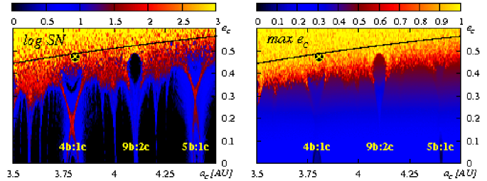
Figure 3.—

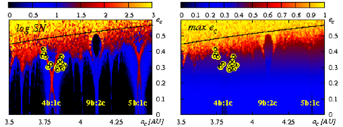
Figure 4.—

Figure 5.—

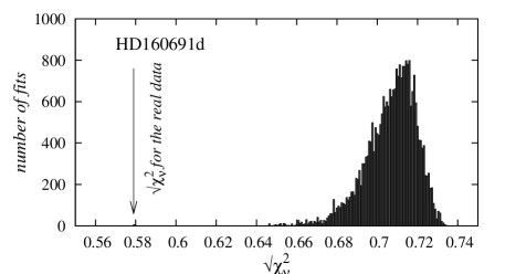
Figure 6.—

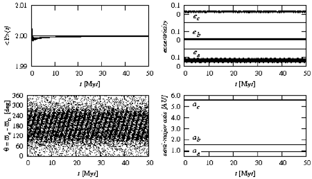
Figure 7.—

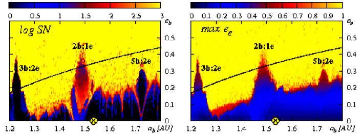
Figure 8.—

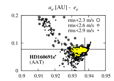
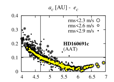
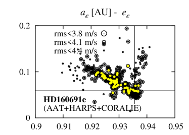
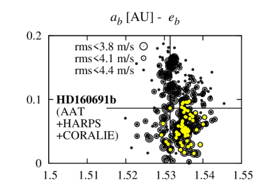
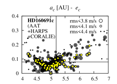
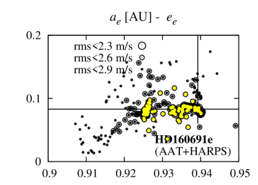
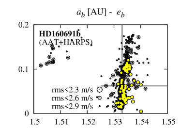
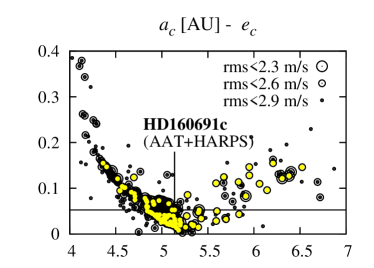
Figure 9.—

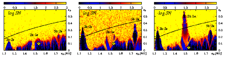
Figure 10.—

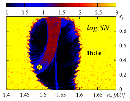
Figure 11.—

References

- Arnold (1978) Arnold, V. I. 1978, Mathematical methods of classical mechanics (Graduate texts in mathematics, New York: Springer, 1978)
- Beaugé et al. (2003) Beaugé, C., Ferraz-Mello, S., & Michtchenko, T. A. 2003, ApJ, 593, 1124
- Bevington & Robinson (2003) Bevington, P. R. & Robinson, D. K. 2003, Data reduction and error analysis for the physical sciences (McGraw-Hill)
- Bouchy et al. (2005) Bouchy, F., Bazot, M., Santos, N. C., Vauclair, S., & Sosnowska, D. 2005, A&A, 440, 609
- Butler et al. (2001) Butler, R. P., Tinney, C. G., Marcy, G. W., Jones, H. R. A., Penny, A. J., & Apps, K. 2001, ApJ, 555, 410
- Butler et al. (2004) Butler, R. P., Vogt, S. S., Marcy, G. W., Fischer, D. A., Wright, J. T., Henry, G. W., Laughlin, G., & Lissauer, J. J. 2004, ApJ, 617, 580
- Butler et al. (2006) Butler, R. P., Wright, J. T., Marcy, G. W., Fischer, D. A., Vogt, S. S., Tinney, C. G., Jones, H. R. A., Carter, B. D., Johnson, J. A., McCarthy, C., & Penny, A. J. 2006, ApJ, 646, 505
- Cincotta & Simó (2000) Cincotta, P. M. & Simó, C. 2000, A&AS, 147, 205
- Charbonneau (1995) Charbonneau, P. 1995, ApJS, 101, 309
- Ford & Gaudi (2006) Ford, E. & Gaudi, B. S. 2006, astroph/0609298
- Goździewski & Konacki (2004) Goździewski, K. & Konacki, M. 2004, ApJ, 610, 1093
- Goździewski & Konacki (2006) Goździewski, K. & Konacki, M. 2006, ApJ, 647, 573
- Goździewski et al. (2003) Goździewski, K., Konacki, M., & Maciejewski, A. J. 2003, ApJ, 594
- Goździewski et al. (2005) —. 2005, ApJ, 622, 1136
- Goździewski et al. (2006) Goździewski, K., Konacki, M., & Maciejewski, A. J. 2006, ApJ, 645, 688
- Goździewski et al. (2005) Goździewski, K., Konacki, M., & Wolszczan, A. 2005, ApJ, 619, 1084
- Goździewski & Migaszewski (2006) Goździewski, K. & Migaszewski, C. 2006, A&A, 449, 1219
- Jones et al. (2002) Jones, H., Butler, P., Marcy, G., Tinney, C., Penny, A., C., M., & B., C. 2002, MNRAS, 337, 1170
- Ji et al. (2003) Ji, J. et al. 2003, Celestial Mech. Dyn. Astr, 74, 113
- Laskar (2000) Laskar, J. 2000, Physical Review Letters, 84, 3240
- Laughlin & Chambers (2001) Laughlin, G. & Chambers, J. E. 2001, ApJ, 551, L109
- Lee et al. (2006) Lee, M. H., Butler, R. P., Fischer, D. A., Marcy, G. W., & Vogt, S. S. 2006, ApJ, 641, 1178
- Lee & Peale (2003) Lee, M. H. & Peale, S. J. 2003, ApJ, 592, 1201
- Lovis et al. (2006) Lovis, C., Mayor, M., Pepe, F., Alibert, Y., Benz, W., Bouchy, F., Correia, A. C. M., Laskar, J., Mordasini, C., Queloz, D., Santos, N. C., Udry, S., Bertaux, J.-L., & Sivan, J.-P. 2006, Nature, 441, 305
- Mayor et al. (2004) Mayor, M., Udry, S., Naef, D., Pepe, F., Queloz, D., Santos, N. C., & Burnet, M. 2004, A&A, 415, 391
- McArthur et al. (2004) McArthur, B. E., Endl, M., Cochran, W. D., Benedict, G. F., Fischer, D. A., Marcy, G. W., Butler, R. P., Naef, D., Mayor, M., Queloz, D., Udry, S., & Harrison, T. E. 2004, ApJ, 614, L81
- McCarthy et al. (2004) McCarthy, C. et al. 2004, ApJ, 617, 575
- Michtchenko & Ferraz-Mello (2001) Michtchenko, T. & Ferraz-Mello, S. 2001, ApJ, 122, 474
- Nauenberg M. (2002) Nauenberg, C. 2002, ApJ, 124, 233
- Pepe et al. (2006) Pepe, F. et al 2006, astro-ph/0608396
- Press et al. (1992) Press, W. H., Teukolsky, S. A., Vetterling, W. T., & Flannery, B. P. 1992, Numerical Recipes in C. The Art of Scientific Computing (Cambridge Univ. Press)
- Psychoyos & Hadjidemetriou (2005) Psychoyos, D. & Hadjidemetriou, J. D. 2005, Celestial Mech. Dyn. Astr., 92, 135
- Rivera & Lissauer (2001) Rivera, E. J. & Lissauer, J. J. 2001, ApJ, 402, 558
- Rivera et al. (2005) Rivera, E. J., Lissauer, J. J., Butler, R. P., Marcy, G. W., Vogt, S. S., Fischer, D. A., Brown, T. M., Laughlin, G., & Henry, G. W. 2005, ApJ, 634, 625
- Santos et al. (2004) Santos, N. C. et al. 2004, A&A, 426, L19
- Smart (1949) Smart, W. M. 1949, Text-Book on Spherical Astronomy (Cambridge Univ. Press)
- Tinney et al. (2006) Tinney, C. G., Butler, R. P., Marcy, G. W., Jones Penny, A. J., McCarthy, C., Carter, B. D., & Fischer, D. 2006, ApJ, 647, 594
- Vogt et al. (2005) Vogt, S. S., Butler, R. P., Marcy, G. W., Fischer, D. A., Henry, G. W., Laughlin, G., Wright, J. T., & Johnson, J. A. 2005, ApJ, 632, 638
- Wright (2005) Wright, J. T. 2005, PASP, 117, 657