Constraints on the Inflationary Expansion from Three Year WMAP, small scale CMB anisotropies and Large Scale Structure Data Sets

Abstract

We present the constraints on inflationary parameters in a flat $\Lambda$CDM universe obtained by WMAP three year data release, plus smaller scale CMB and two LSS data sets, 2dF and SDSS (treated separately). We use a Markov Chain Monte Carlo (MCMC) technique combined with an analytic description of the inflationary spectra in terms of the horizon flow functions (HFF). By imposing a consistency condition for the tensor-to-scalar ratio, we study the constraints both on single field standard inflation and on inflation with the violation of the null energy condition, which leads to a blue spectrum for gravitational waves. For standard inflation, the constraint on the tensor-to-scalar ratio we obtain from CMB data and 2dF05 is: $r_{0.01}<0.26$ at 2 $\sigma$ cl. Without the consistency condition between the tensor-to-scalar ratio and the tensor slope, the constraints on the tensor amplitude is not significantly changed, but the constraints on the HFFs are significantly relaxed. We then show that when the third HFF $\epsilon_{3}$ is allowed to be non-zero and to be of order unity, a large negative (at $2\sigma$) value for the running of the scalar spectral index in standard inflation is found in any set of data we consider.

Introduction

Inflation is the most promising paradigm for understanding the initial conditions for cosmic structure formation and the pattern of anisotropies in temperature and polarization of the cosmic microwave background (CMB). Its predictions for the simplest case of a single scalar field model with a nearly scale-invariant spectrum of curvature and tensor perturbations are in good agreement with most of the observational data.

Among observations, data on CMB anisotropies have been the most selective for inflation, starting from COBE-DMR [1] to the NASA mission presently in operation WMAP [2]. The WMAP first-year data [3, 4] complemented with smaller scale data started to discriminate among the inflationary models and to constrain the possibility that the spectra may have not a pure power-law shape [5, 6].

In this paper we compare inflationary predictions with WMAP three year data release [7, 8, 9] plus smaller scale CMB data (which we shall denote collectively as CMBsmall), such as CBI [10], ACBAR [11], VSA [12] and B2K [13, 14, 15]. We shall also use separately two LSS data sets, SDSS [16] and 2dF [17, 18].

We compare inflationary predictions with observations, by adopting a parametrization of the primordial power spectra (PS henceforth) of curvature and tensor perturbations as:

$$P_{S}(k) = A_{S}\,e^{(n_{S}-1)\ln(k/k_{*})+\alpha_{S}\ln^{2}(k/k_{*})/2}\,,$$

$$P_{T}(k) = A_{T}\,e^{n_{T}\ln(k/k_{*})+\alpha_{T}\ln^{2}(k/k_{*})/2}$$ (1)

where $i={\rm S\,,T}$ stands for scalar and tensor, respectively, $k_{*}$ is the pivot scale. We shall use $A_{i},n_{i},\alpha_{i}$ in terms of of the Hubble parameter $H$ and the horizon flow functions $\epsilon_{i}$ (HFF henceforth) evaluated at the pivot scale $k_{*}$. At the present state of the art, the PS of primordial perturbations in most of the single field inflationary models depend only on the physics at the Hubble crossing since adiabaticity on large scale is preserved.

The HFFs are defined as $\epsilon_{1}=-\dot{H}/H^{2}$ and $\epsilon_{i+1}\equiv\dot{\epsilon}_{i}/(H\epsilon_{i})=(d\epsilon_{i}/d\,N)/\epsilon_{i}$ with $i\geq 1$ and $N$ the number fo e-folds ($dN=Hdt$) [20]. For a Klein-Gordon scalar field $\phi$, $H$ and $\epsilon_{i}$ are related to the potential and its derivatives as:

$$V = 3\,M_{\rm Pl}^{2}\,H^{2}\left(1-\frac{\epsilon_{1}}{3}\right),$$

$$V_{\phi} = -3\,\sqrt{2}\,M_{\rm Pl}\,H^{2}\,\epsilon_{1}^{1/2}\,\left(1-\frac{\epsilon_{1}}{3}+\frac{\epsilon_{2}}{6}\right),$$

$$\frac{V_{\phi\phi}}{3H^{2}} = 2\epsilon_{1}-\frac{\epsilon_{2}}{2}-\frac{2\epsilon_{1}^{2}}{3}+\frac{5\epsilon_{1}\epsilon_{2}}{6}-\frac{\epsilon_{2}^{2}}{12}-\frac{\epsilon_{2}\epsilon_{3}}{6}\,,$$ (2)

where $M_{\rm Pl}=(8\pi G)^{-1/2}\simeq 2.4\times 10^{18}$ Gev is the reduced Planck mass. By comparing constraints on $H\,,\epsilon_{i}$ derived by observations, the shape of the inflationary potential can be constrained through Eqs. (2).

We use the most advanced analytic descriptions of inflationary spectra which relate $(A_{i},n_{i},\alpha_{i})$ to $(H,\epsilon_{j})$. These expressions are obtained by the Green’s function method (henceforth GFM) [21, 22] and by the method of comparison equations (henceforth MCE) [23]. These two methods provide a description of cosmological perturbations spectra up to second order in the HFF, allowing a good accuracy also in inflationary models where the HFF are not so small or constant in time, i.e. the slow-roll condition is not well satisfied [22, 23, 24]. Note that the GFM and MCE methods predict the same PSs at ${\cal O}(\epsilon_{j})$, but differences of percent order arise in the coefficients of ${\cal O}(\epsilon_{j}^{2})$ terms [23].

In this paper we address several points of current interest in comparing inflationary preditions with observations. At first order in HFFs we update the analysis of Leach and Liddle [6] to WMAP3 [7, 8, 9] and to 2dF05 [18]. At second order in HFFs, we first show how the large running found by the WMAP team [29, 5, 9] is recovered by using the PS parametrization in terms of the HFFs. We also give a model-independent constraint on the tensor amplitude by considering the tensor-to-scalar ratio as a free parameter and not given in terms of the tensor spectral index. We then study the constraints on inflationary models which violate the null energy condition (NEC) and predict a blue spectrum for gravitational waves [25].

Our paper is organized as follows. In section II we present our methodology and in section III the constraints on cosmological parameters by restricting the parametrization for the spectra at first order in HFFs for standard inflationary models. In section III we relax the assumption that the inflaton is a Klein-Gordon (KG henceforth) scalar field and we leave the tensor-to-scalar ratio as a free parameter. In section IV we compare the constraints on inflationary models with a blue spectrum for gravitational waves with standard inflationary models. In section V we present the results obtained allowing running(s) of the spectral indices in standard inflationary models, i.e. taking into account spectra to second order in HFFs. In section VI we conclude.

1 Methodology

We use the publicly available Markov Chain Monte Carlo (MCMC) package [26] which makes use of the Einstein-Botzmann code CAMB [27] for the computation of theoretical CMB anisotropies PSs and transfer functions. We restrict ourselves to flat spatial sections and to three species of massless neutrinos. We use as initial conditions for cosmological fluctuations the growing adiabatic mode. We include the CMBsmall data set as by default implemented in COSMOMC. Note that small scale data by the same experiments have been used by the WMAP team in Ref. [9], although there may be additional cross-correlations between the data sets which we consider and WMAP3 data. We restrict our analysis to linear transfer functions and therefore the LSS data are automatically truncated by the MCMC to $k_{\rm cut}/h\simeq 0.15$ ($0.2$) for 2dF (SDSS). The convergence diagnostic on runs with multiple chains is the R statistic by Gelman and Rubin implemented in the MCMC.

We use the $\ln(k/k_{*})$ expansion of the logarithm of the parametrizations in Eqs. (1), in order to avoid that the spectrum becomes negative for some values of the inflationary parameters explored by MCMC [22]. According to Eqs. (1), the $\ln(k/k_{*})$ expansion of the power spectra is:

$$\ln{P(k)\over P_{0}(k_{*})}=b_{0}+b_{1}\ln\left(k\over k_{*}\right)+\frac{b_{2}}{2}\ln^{2}\left(k\over k_{*}\right)+\dots.$$ (3)

and we use both the GFM [21] and MCE [22] to relate the coefficients $b$s to the HFFs. The coefficients for the scalar spectrum are:

$$b_{{\rm S}0} = -2\left(C+1\right)\epsilon_{1}-C\epsilon_{2}+\left(-2C+{\textstyle\frac{\pi^{2}}{2}}-7\right)\epsilon_{1}^{2}$$ (4)

$$+\left({\textstyle\frac{\pi^{2}}{8}}-1\right)\epsilon_{2}^{2}+\left(-X^{2}-3X+{\textstyle\frac{7\pi^{2}}{12}}-7+2\Delta_{{\rm S}0}\right)\epsilon_{1}\epsilon_{2}$$

$$+\left(-{\textstyle\frac{1}{2}}X^{2}+{\textstyle\frac{\pi^{2}}{24}}+\Delta_{{\rm S}0}\right)\frac{d\epsilon_{2}}{dN}\,$$

$$b_{{\rm S}1} \equiv n_{S}-1=-2\epsilon_{1}-\epsilon_{2}-2\epsilon_{1}^{2}-\left(2\,X+3\right)\,\epsilon_{1}\,\epsilon_{2}-X\,\frac{d\epsilon_{2}}{dN}\,$$ (5)

$$b_{{\rm S}2} \equiv \alpha_{S}=-2\epsilon_{1}\epsilon_{2}-\frac{d\epsilon_{2}}{dN},$$ (6)

and for tensors are:

$$b_{{\rm T}0} = -2\left(C+1\right)\epsilon_{1}+\left(-2C+{\textstyle\frac{\pi^{2}}{2}}-7\right)\epsilon_{1}^{2}$$ (7)

$$+\left(-X^{2}-2X+{\textstyle\frac{\pi^{2}}{12}}-2+\Delta_{{\rm T}0}\right)\epsilon_{1}\epsilon_{2},$$

$$b_{{\rm T}1} \equiv n_{T}=-2\epsilon_{1}-2\epsilon_{1}^{2}-2\,\left(X+1\right)\,\epsilon_{1}\,\epsilon_{2},$$ (8)

$$b_{{\rm T}2} \equiv \alpha_{T}=-2\epsilon_{1}\epsilon_{2},$$ (9)

where $C\equiv\ln 2+\gamma_{\rm E}-2\approx-0.7296$ ($\gamma_{\rm E}$ is the Euler-Mascheroni constant) and $d\epsilon_{2}/dN=\epsilon_{2}\epsilon_{3}$. At second order the next-to-leading coefficients depend on the method of approximation used to study cosmological perturbations during inflation: $X=C$ and $\Delta_{{\rm S}0}=\Delta_{{\rm T}0}=0$ are obtained within the GFM [21, 22]; $X=D\equiv\frac{1}{3}-\ln 3\approx-0.7652$, $\Delta_{{\rm S}0}=(D-C)(D+\ln\,2)-1/18$, $\Delta_{{\rm T}0}=2D(D-C)-1/9$, within the MCE [23]. We therefore implement the above expansion in a modified version of the inflationary routines developed by Samuel Leach and public at http://astronomy.sussex.ac.uk/$\sim$sleach/inflation/camb_inflation.html.

As pivot scale we choose $k_{*}=0.01\,{\rm Mpc}^{-1}$ as in [6] (see however [28]); this choice differs from those by the WMAP team ($k_{*}=0.002\,{\rm Mpc}^{-1}$ [5, 9] and $k_{*}=0.05\,{\rm Mpc}^{-1}$ [29]) and is better placed at the center of the range of wavenumbers probed by cosmological perturbations studied in the linear regime. Although the CMB spectrum includes at least a convolution of the power-spectrm with spherical Bessel functions, an effective pivot $\ell_{*}$ corresponding to $k_{*}$ can be defined [30, 22]:

$$k_{*}=\frac{3}{2}\frac{h\sqrt{\Omega_{\rm m}}}{1+0.084\ln\Omega_{\rm m}}\ell_{*}\times 10^{3}\,{\rm Mpc}^{-1}\,.$$ (10)

Since $\ell_{*}\simeq 145$ corresponding to $k_{*}=0.01\,{\rm Mpc}^{-1}$ does not represent an interesting reference scale to measure the tensor-to-scalar ratio, we shall also quote in our results both $r_{k_{*}}$ and the ratio of tensor to scalar contribution to $C_{\ell}$ and $l=10$, denoted by $R_{10}$ ($\equiv C_{10}^{T}/C_{10}^{S}$).

As parameter describing reionization we shall vary the redshift $z_{\rm re}$, which is related to the optical depth $\tau$ by an integration over the redshift $z$ [26]

$$\tau=\sigma_{T}\int_{0}^{z_{\rm re}}dz\frac{n_{e}(z)}{H(z)(1+z)^{2}}\,,$$ (11)

with $\sigma_{T}$ as the Thompson cross section and $n_{e}$ is the electron density number. As for the tensor-to-scalar ratios $r$ and $R_{10}$, we also give the constraints on $\tau$ as a derived parameter.

2 First Order HFF Results

In this section we explore the constraints for a model in which the inflaton is described by a Klein-Gordon scalar field and the spectra in Eqs. (3) are taken to first order in HFFs (i.e. $b_{{\rm S}2}=b_{{\rm T}2}=0$). When the inflaton is described by a Klein-Gordon scalar field the tensor-to-scalar ratio is not a free parameter, but is given by the so-called consistency condition which is:

$$\frac{P_{0\,T}}{P_{0\,S}}=16\epsilon_{1}\,.$$ (12)

In this case we vary $7$ free parameters:

$$\{\Omega_{b}\,h^{2},\Omega_{cdm}h^{2},H_{0},10^{10}A_{\rm S},z_{re},\epsilon_{1},\epsilon_{2}\}\,,$$ (13)

where $\Omega_{b}\,,\Omega_{cdm}$ are baryon and cold dark matter densities, $H_{0}$ is the present Hubble parameter, $h=H_{0}/(100\,{\rm km\,s}^{-1}\,{\rm Mpc}^{-1})$, $A_{\rm S}(k_{*})$ is the amplitude of super-Hubble curvature perturbation deep in the radiation era, $\epsilon_{1}\,,\epsilon_{2}$ are the first two HFFs. The prior on these parameters are: $0.005<\Omega_{b}h^{2}<0.1$, $0.01<\Omega_{cdm}<0.99$, $40<H_{0}/{\rm kms}^{-1}{\rm Mpc}^{-1}<100$, $4<z_{re}<30$ as in [6] , $10^{-4}<\epsilon_{1}<0.1$; $-0.25<\epsilon_{2}<0.2$

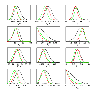
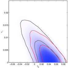
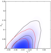
The one dimensional posterior marginalized probability distributions obtained from a Markov chain of (at least) $10^{5}$ elements (which uses the covariance matrix of a preliminary chain) for sampled and derived parameters are shown in Fig. 1,2 and in Table 1. We compare the results obtained by using the first year and the three years of WMAP data (plus CMBsmall and 2dF02 [17]), as well as the results of the three years of WMAP data and CMBsmall with different LSS data sets (2dF02 [17], SDSS [16] and 2dF05 [18]). Different estimates of cosmological parameters obtained with different LSS data sets are very known (see Table 6 of [9]) and may be due to different selection of the SDSS and 2dF surveys: this is the reason why we do not combine different LSS data sets.

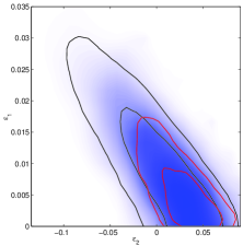
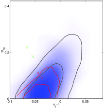
One of the main results of WMAP3, i.e. a better estimate (and different from WMAP1) of reionization, has changed the value of the scalar spectral index $n_{S}$. By combining with CMBsmall plus 2dF02, WMAP3 fully marginalized $2\sigma$ value is $n_{S}=0.960\pm^{0.033}_{0.032}$ (compared to the WMAP1 correspondent value $n_{S}=0.979\pm^{0.056}_{0.035}$). As is clear from the right panel of Figs. 3,4, without marginalizing on the tensor-to-scalar ratio, a pure Harrison-Zeldovich spectrum for scalar perturbations with no tensors ($n_{s}=1\,,r=0$) is disfavoured at more than $2\sigma$ by the combination of CMB data with 2dF02 or SDSS, but is within $2\sigma$ for CMB data plus 2dF05. Another interesting result we find is that inflationary models predicting $n_{S}=1$ ($\epsilon_{2}=-2\epsilon_{1}$) and tensors are also disfavoured at $2\sigma$ by the same data sets for which the HZ spectrum is disfavoured with the same cl (again, this is not true for CMB data plus 2dF05). As shown by Fig. 4, this effect is due to the inclusion of small scale CMB datasets [10, 11, 12, 13, 14, 15]. Note from Fig. 4 how our results on WMAP3 + SDSS agree with previous analysis with the same data sets [31, 32]. By comparing our results to Fig. 1 of [33] where WMAP1 results were reported, we see that models with a natural exit from inflation (the region $\epsilon_{2}>0$) are now preferred by WMAP3.

Figure 1: One dimensional marginalized probabilities for cosmological parameters obtained by WMAP1+CMBsmall+2dF02 (black), WMAP3+CMBsmall plus 2dF02 (red) or plus 2dF05 (green).

Figure 2: One dimensional marginalized probabilities for cosmological parameters obtained by using WMAP3+CMBsmall (black), WMAP3+CMBsmall plus 2dF02 (red) or plus SDSS (green).

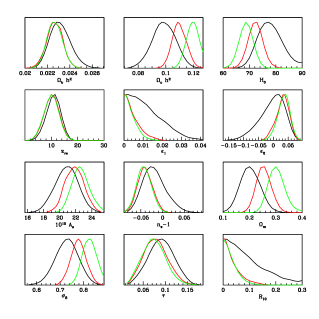Our analysis tightens the previous bounds on $\epsilon_{1}$ [6, 37]. By combining WMAP3+CMBsmall with 2dF02 (SDSS) the $2\sigma$ cl constraint (obtained without marginalizing on $\epsilon_{2}$) is $\epsilon_{1}<0.017$ ($\epsilon_{1}<0.013$). These limits translate on the derived parameter $R_{10}<0.14$ ($R_{10}<0.10$) obtained without marginalized on $n_{S}$. The current bound on $\epsilon_{1}$ is almost half of the WMAP1 constraint, $\epsilon_{1}<0.031$ . From this result we obtain that the bound on the Hubble scale of inflation driven by a KG scalar field derived by WMAP3+CMBsmall+2dF02: by using the values (not fully marginalized) in Fig. (3) we obtain $H/m_{\rm pl}<1.1\times 10^{-5}$ which improves the values previously found [6, 37] (and implies $(V_{*}^{\rm infl})^{1/4}<2.4\times 10^{16}$ GeV).

The impact of WMAP3 on simple monomial chaotic models with $V(\phi)\propto\phi^{n}$ strengthens the trend already present in WMAP1. For these models, the HFFs are given in terms of the number of e-folds to the end inflation $\Delta N$ as: $\epsilon_{1}\simeq n\epsilon_{2}/4\simeq n/(4\Delta N)$. The quartic model is now disfavoured at more than $3\sigma$ (although the agreement of the amplitude of scalar perturbations in such model is not robust with respect to the preheating mechanism [34]). A massive inflaton is in agreement with observations, although it moves in the $2\sigma$ cl with WMAP3 data.

Power-law inflation [35] obtained by an exponential potential $V(\phi)=V_{0}\exp(-\lambda\phi/M_{\rm Pl})$ ($\lambda=\sqrt{2/p}$ with $a\sim t^{p}$) stay on the line $\epsilon_{2}=0$ in the ($\epsilon_{2}\,,\epsilon_{1}$) plane. From the left panel of Fig. 3 and from the relation $\epsilon_{1}=1/(p-1)$ we obtain $p>60$ at $2\sigma$ cl (compared with $p>53$ at $1\sigma$ cl of Ref. [6]). An interesting issue is the appearance of an upper bound (at $2\sigma$ cl) starts to appear from the left panel of Fig. 3, i.e. $p<500$ for WMAP3+CMBsmall+2dF02 (or SDSS): as is clear from Fig. 4, also this limit may depend on the inclusion of small scale CMB data and for its significativity hold the same reasoning made above for the $n_{s}=1$ spectrum. Note however that the fully marginalized (on non-zero values of $\epsilon_{2}$) value for $\epsilon_{1}$ reported in Table I does not have any non-zero lower bound. This upper limit for $p$, if confirmed by future data, can become important in constraining the number of fields which support assisted inflation [36], a particle physics realization of power-law inflation. The constraints on the exponent of the potential at $2\sigma$ cl are $0.063<\lambda<0.18$.

Parameter	WMAP1+CMBsmall+2dF02	WMAP3+CMBsmall+2dF02	WMAP3+CMBsmall+2dF05
$\Omega_{b}h^{2}$	$0.0236^{+0.0010}_{-0.0010}$	$0.0226^{+0.0007}_{-0.0006}$	$0.0228^{+0.0007}_{-0.0008}$
$\Omega_{cdm}h^{2}$	$0.113^{+0.006}_{-0.006}$	$0.110^{+0.005}_{-0.005}$	$0.105^{+0.005}_{-0.005}$
$H_{0}$	$73.4^{+1.3}_{-1.7}$	$72.3^{+1.1}_{-1.2}$	$74.3^{+2.5}_{-2.3}$
$z_{re}$	$11.7^{+1.9}_{-1.5}$	$10.1^{+1.2}_{-1.1}$	$10.0^{+1.6}_{-0.9}$
$\epsilon_{1}$	$<0.024$	$<0.013$	$<0.016$
$\epsilon_{2}$	$0.001^{+0.038}_{-0.037}$	$0.03^{+0.02}_{-0.02}$	$0.02^{+0.02}_{-0.02}$
$10^{10}A_{\rm s}$	$22.5^{+1.6}_{-1.6}$	$21.8^{+1.2}_{-1.1}$	$21.3^{+1.3}_{-1.3}$
$n_{\rm s}-1$	$-0.021^{+0.025}_{-0.026}$	$-0.040^{+0.017}_{-0.017}$	$-0.035^{+0.007}_{-0.009}$
$\Omega_{m}$	$0.256^{+0.032}_{-0.031}$	$0.255^{+0.025}_{-0.025}$	$0.232^{+0.020}_{-0.021}$
$\sigma_{8}$	$0.82^{+0.04}_{-0.04}$	$0.78^{+0.03}_{-0.03}$	$0.76^{+0.03}_{-0.04}$
$\tau$	$0.10^{+0.04}_{-0.04}$	$0.078^{+0.027}_{-0.026}$	$0.080^{+0.031}_{-0.034}$
$R_{10}$	$<0.22$	$<0.10$	$<0.13$

Table 1: Mean values and $1\sigma$ constraints for the $7$ basic parameters and other $5$ derived quantities from the first and three year WMAP release combined with the two release of 2dF plus CMBsmall. For $\epsilon_{1}$ and $R_{10}$ the 2$\sigma$ upper bounds are given.

Figure 3: Constraints by using WMAP3 (red) vs WMAP1 (black) plus CMBsmall+2dF on ($\epsilon_{2}\,,\epsilon_{1}$) and ($n_{s}-1\,,R_{10}$) planes at $1\sigma$ and $2\sigma$ level. On the right panel, the inflationary predictions for $V(\phi)=\lambda\phi^{4}/4$ (green) and for $V(\phi)=m^{2}\phi^{2}/2$ (red) with $45<\Delta N<55$ are shown for comparison.

Figure 4: Constraints by using WMAP3+SDSS (black) vs WMAP3+CMBsmall+SDSS (red) on ($\epsilon_{2}\,,\epsilon_{1}$) and ($n_{s}-1\,,R_{10}$) planes at $1\sigma$ and $2\sigma$ level. The right panel shows how the inclusion of small scale CMB data drives the spectral scalar index towards red values, disfavouring at just 2$\sigma$ cl the $n_{s}=1$ line. The constraints on $n_{S}$ we obtain from WMAP3+SDSS are in complete agreemente with [31, 32].

3 Relaxing the standard consistency condition

We now discuss the bounds obtained by relaxing the consistency condition (12) and by therefore varying $8$ parameters (the $7$ of Eq. (13) plus the tensor-to-scalar ratio $r_{0.01}$ at the pivot scale $k_{*}=0.01{\rm Mpc}^{-1}$). From a theoretical point of view, this means that we are not specifying the Lagrangian $p(\phi,X)$ for the inflaton $\phi$ and its kinetic term $X=-\nabla_{\mu}\phi\nabla^{\mu}\phi/2$, but we are restricting ourselves to inflationary spectra at first order in HFF. In this way the consistency condition in Eq. (12) is modified by the speed of sound $c_{S}$ for the inflaton [38]:

$$\frac{P_{0\,T}}{P_{0\,S}}=-8c_{S}n_{T}\,,\quad{\rm with}\quad c_{S}^{2}=\frac{\partial p}{\partial X}\,,$$ (14)

whereas the spectral indices in Eqs. (6,9) are not modified by $c_{S}$ at first order in HFF for constant $c_{S}$ [40]. Our analysis with a tensor-to-scalar ratio unrelated to the tensor spectral index also applies to inflation driven by more than one scalar field, by assuming only curvature perturbations after nucleosynthesis (i.e. that isocurvature perturbations generated during inflation have completely transferred to the adiabatic mode when fluctuations are initialized in the Einstein-Boltzmann code).

Figure 5: Two dimensional contours at $1\sigma$ and $2\sigma$ level obtained by WMAP3+CMBsmall+2dF02. The plots reported from left to right are $(\epsilon_{2}\,\epsilon_{1})$, $(n_{S}-1\,,R_{10})$, $(16\,\epsilon_{1}\,,r)$, respectively. In the plane $(16\,\epsilon_{1}\,,r)$, the red line describing the consistency condition $r=16\epsilon_{1}$ is also drawn for comparison.

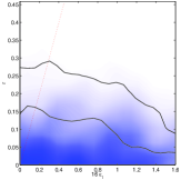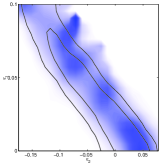
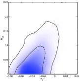
The two dimensional constraints for relevant parameters are presented in Fig. (5). The constraints on the ($\epsilon_{1}\,,\epsilon_{2}$) plane become looser than in the previous section, since $\epsilon_{1}$ is now unrelated to the tensor-to-scalar ratio. Without marginalizing on the scalar spectral index, we obtain $r<0.29$ (or $R_{10}<0.185$) at 2$\sigma$ cl, a bound weaker than the one obtained by imposing the standard consistency condition in Eq. (12) ($r<0.27$ or $R_{10}<0.14$, see previous section). Note that inflation driven by KG scalar field (i.e. $c_{S}=1$) is fully consistent with present data.

4 NEC violating Inflation

Inflation may occur with a violation of the null energy condition (NEC) [25], i.e. with $\epsilon_{1}<0$. Since $n_{T}=-2\epsilon_{1}$, a prediction of NEC violating inflation is a blue spectrum for gravitational waves. A similar blue spectrum for gravitational waves may occur also in scalar-tensor theories and $f(R)$ gravity theories which are NEC violating in the Einstein frame conformally related to the original Jordan one. In order to remain with $3$ inflationary parameters, we shall restrict ourselves to a simple model, just changing the sign of the kinetic term of standard inflation, which leads to relation $r\simeq-16\epsilon_{1}$ in the analysis [41]. The prior used is $-10^{-4}<\epsilon_{1}<-0.1$.

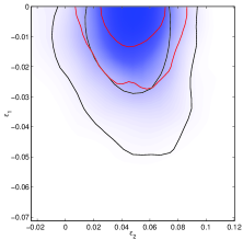
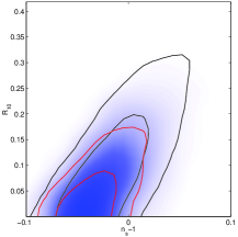
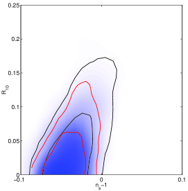
The constraints on the ($\epsilon_{2}\,,\epsilon_{1}$) for $\epsilon_{1}<0$ are presented in the left panel of Fig. (6). The contours on ($\epsilon_{2}\,,\epsilon_{1}$) for NEC violated inflation are completely different from standard inflation, although the amount of tensor is slightly loosely constrained with respect to standard inflation because of the the blue slope for gravitational waves, as can be seen in Fig. (7). The best fits for standard inflation and for NEC violating inflation have the same value for $\chi^{2}$ ($=5673$) with WMAP3+CMBsmall+2dF02.

From the ($\epsilon_{2}\,,\epsilon_{1}$) plane, it can be seen that an exponential potential (described by the $\epsilon_{2}=0$ line) is disfavoured at more than $2\sigma$ cl. A potential $V(\phi)\sim\exp\left(\bar{\epsilon}_{2}\phi^{2}/M_{\rm pl}^{2}\right)$ with $0.02\lesssim\bar{\epsilon}_{2}\lesssim 0.08$ is consistent with the data.

Figure 6: WMAP3 (red) vs WMAP1 (black) $1\sigma$ and $2\sigma$ contours on ($\epsilon_{2}\,,\epsilon_{1}$) (left) and ($R_{10}\,,n_{s}-1$) for NEC violating inflation. The other data used are CMBsmall and 2dF02.

Figure 7: Standard inflation (red) vs NEC violating inflation (black) on the ($n_{S}-1\,,R_{10}$) at $1\sigma$ and $2\sigma$ level.

5 Second Order HFF Results

We now allow $b_{{\rm S}\,2}\,,b_{{\rm T}\,2}\neq 0$ in Eq. (3), which, according to inflationary predictions, is equivalent to take into account terms which are quadratic in HFFs. Inflationary models in which the slow-roll condition is not well satisfied can be described analitycally with better accuracy by including the spectra at second order in HFFs [22, 23, 24].

Let us first try to predict what may happen by inserting the PSs in Eq. (3) which allow running with respect to the pure power-law PSs analyzed in Section III: at the price of one additional parameter, the input scalar and tensor PSs are now paraboles in $\ln(k/k_{*})$, and not straight lines. It is expected that the $7$ parameters used in Section III change their mean value and broaden their variance in presence of the running, the additional parameter. Having in mind the degeneracy in cosmological parameters, it is also possible that the best-fit model with runnings may be fairly different from the best-fit model without runnings. Within our analysis, we shall see that both these possibilities indeed occur with different LSS data sets.

WMAP 3yr analysis included the running of the scalar spectral index as an additional parameter [9], neither enforcing a self-consistent tensor-to-scalar ratio to second order in HFFs nor including a running for the tensor spectral index. See also other studies of the running of the spectral index for WMAP1 [42] and WMAP3 [43].

Figure 8: One dimensional mean likelihhods (dashed) and marginalized probabilities (solid) for $\epsilon_{1}\,,\epsilon_{2}\,,\epsilon_{3}$ using a prior $-0.2\leq\epsilon_{3}\leq 0.2$ and the GFM. We show for comparison results from WMAP1 (red) and WMAP3 (black) plus CMBsmall+2dF02.

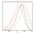
We show in Fig. (8) the mean likelihoods and marginalized probabilities for $\epsilon_{1}\,,\epsilon_{2}\,,\epsilon_{3}$ with a prior $[-0.2\,,0.2]$ on $\epsilon_{3}$ obtained by the two WMAP releases. The results obtained are qualitatively in agreement with [6] (for WMAP1) and [37] (for WMAP3), although the sets of auxiliary data used are not the same. It is clear from Fig. (8) and Eqs. (6) that such prior constrains $|\alpha_{S}|\lesssim 0.01$, although there is a tendency to favour positive values for $\epsilon_{3}$, in particular for WMAP3 (as also pointed out in [37]).

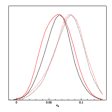
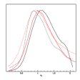
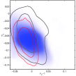
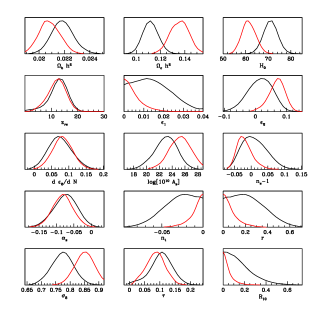
In order to have a non trivial result for $\epsilon_{3}$ it is crucial to consider a broader prior on this parameter. The justification for this broader prior for $\epsilon_{3}$ is its appearance in Eqs. (3-10) not at linear level, but always multiplied by $\epsilon_{2}$. The second order formalism is limited by $\epsilon_{1}\epsilon_{2}\,,\epsilon_{2}\epsilon_{3}<<1$ and not by $\epsilon_{3}<<1$ (see also [24] for a similar claim). By repeating the same analysis with a much broader prior , we find more definite preferred values around $\epsilon_{3}\sim 1$, as can be seen from Fig. (9). In the right panel of Fig. (9) we show how the statistical evidence for running has increased from WMAP1 to WMAP3, although remaining still weak.

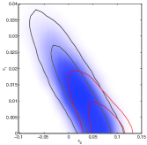
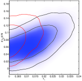
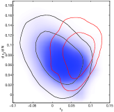
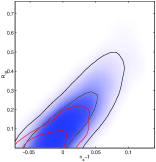
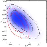
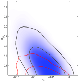
The dependence of $\ln(P(k)/P_{0}(k_{*}))$ in Eq. (3) and of the coefficients $b_{{\rm S\,,T}i}$ in Eqs. (4-10) on $d\epsilon_{2}/dN$ ($=\epsilon_{2}\epsilon_{3}$) is the reason for a very inefficient exploration of runnings of the spectral indexes by the MCMC with basic parameter $\epsilon_{3}$. We find much more efficient sampling directly on $d\epsilon_{2}/dN=\epsilon_{2}\epsilon_{3}$ rather than on $\epsilon_{3}$. We present results on chains obtained sampling on $\epsilon_{2}\epsilon_{3}$ with prior $[-0.5\,,0.5]$ in Table 2 and Figs. 9-10.

Figure 9: First three panels: one dimensional mean (dashed) and marginalized (solid) likelihoods for $\epsilon_{1}\,,\epsilon_{2}\,,\epsilon_{3}$ (left, middle and right panel, respectively) obtained by using the two different analytic approximation for the inflationary power spectra with WMAP3 + CMBsmall + SDSS: GFM (black) and MCE (red). The last panel on the right shows the two dimensional constraints on the ($n_{S}-1,\alpha_{S}$) plane by using the GFM for WMAP1 (black) and WMAP3 (red) plus CMBsmall and SDSS.

Parameter	WMAP3+CMBsmall+2dF05
$\Omega_{b}h^{2}$	$0.0218^{+0.0009}_{-0.0008}$
$\Omega_{cdm}h^{2}$	$0.112^{+0.006}_{-0.006}$
$H_{0}$	$71.0^{+2.7}_{-2.7}$
$z_{re}$	$12.6^{+1.7}_{-1.0}$
$\epsilon_{1}$	$<0.031$
$\epsilon_{2}$	$0.015^{+0.020}_{-0.018}$
$\epsilon_{2}\epsilon_{3}$	$0.076^{+0.033}_{-0.033}$
$10^{10}A_{\rm s}$	$23.0^{+1.7}_{-1.7}$
$n_{\rm s}-1$	$0.010^{+0.038}_{-0.036}$
$\alpha_{\rm s}$	$-0.076^{+0.032}_{-0.033}$
$\sigma_{8}$	$0.77^{+0.04}_{-0.03}$
$\tau$	$0.10^{+0.04}_{-0.03}$
$R_{10}$	$<0.40$

Table 2: Mean values and $1\sigma$ constraints for the $8$ basic parameters and other $5$ derived quantities from WMAP three year data + CMBsmall + 2dF05. Note that for $\epsilon_{1}$ and $R_{10}$ the 2$\sigma$ upper bounds are given. The $2\sigma$ constraints on running of the spectral index is: $-0.141<\alpha_{\rm S}<-0.013$.

Figure 10: One dimensional marginalized likelihoods for $8$ basic parameters and $7$ derived parameters obtained by the GFM formula. We show for comparison the constraints by using WMAP3+CMBsmall plus 2dF05 (black) or plus SDSS (red).

Figure 11: Constraints by using SDSS (red) vs 2dF05 (black) plus WMAP3+CMBsmall on (from left to right and top to bottom) ($\epsilon_{2}\,,\epsilon_{1}$), ($\epsilon_{1}\,,d\epsilon_{2}/dN$) ($n_{s}-1\,,R_{10}$), ($n_{s}-1\,,\alpha_{s}$), ($\alpha_{s}\,,R_{10}$), ($\alpha_{s}\,,\alpha_{t}$), planes at $1\sigma$ and $2\sigma$ level.

At $1\sigma$ we obtain the fully marginalized value of the running of the scalar spectral index $\alpha_{\rm S}=-0.076^{+0.032}_{-0.033}$ ($-0.082^{+0.028}_{-0.028}$) for WMAP3+CMBsmall+2dF05 (SDSS). The $2\sigma$ constraint is $-0.141<\alpha_{\rm S}<-0.013$ ($-0.142<\alpha_{\rm S}<-0.028$) for WMAP3+CMBsmall+2dF05 (SDSS). We note that the best-fit cosmological models obtained by 2dF05 and SDSS are different, enlarging the difference between the two LSS data sets already seen in section III: SDSS prefers a very low value for $H_{0}$ (as also reported in [44]) and the best-fit cosmological model with running is consistent with the one without running only at $2\sigma$. The cosmological models with and without running for 2dF05 are consistent at $1\sigma$: allowing running for the spectral indexes the constraint on $r<0.26$ for 2dF05 is significantly related to $r<0.50$ at $2\sigma$ cl.

Since $\epsilon_{2}\epsilon_{3}$ enters only in the scalar running, the magnitude of the running of the tensor spectral index is constrained at posteriori to be $|\alpha_{T}|\sim{\cal O}(10^{-3}-10^{-4})$, as is also clear from Eqs. (9) and from Fig. (10).

Although our combination of data sets and our method of constraining inflationary parameters differ from those used by the WMAP team [9], our results are in agreement with those reported in [9] for WMAP3 plus other small scale CMB data sets.

6 Conclusions

We have analyzed the observational constraints from CMB and LSS on the inflationary expansion. By parametrizing the inflationary spectra as power-law (i.e. to first order in slow-roll parameters), we have updated the WMAP1 constraints of Ref. [6]: the better determination of reionization obtained by the 3 year data release disfavour now both the Harrizon-Zeldovich model (with no tensor) as inflationary models predicting $n_{s}=1$ with respect to the first year data. Our analysis shows that models with a natural exit from inflation (which stay in the $\epsilon_{2}>0$ region of the $(\epsilon_{2}\,,\epsilon_{1})$ plane according to [33]) are now favoured by WMAP3.

When running is included, we have shown how the prior on $\epsilon_{3}$ plays a crucial role in re-obtaining the WMAP team results within an analysis employing analytic power-spectra depending on ($H\,,\epsilon_{i}$) with $i=1-3$. Only allowing a broad prior on $\epsilon_{3}$ a fairly large negative running in agreement with the WMAP results is obtained. We have found that is more convenient to use $d\epsilon_{2}/dN=\epsilon_{2}\epsilon_{3}$ rather than $\epsilon_{3}$. The value for the running $\alpha_{S}$ found here implies $\alpha_{S}\ln(k/k_{*})/2>(n_{S}-1)$ for Fourier modes far from the pivot scale. It would be therefore interesting to perform a comparison of data with inflationary predictions at third order in the HFF. Note that the value of the running found here is different from zero at $\sim 2\sigma$ level, and its constraints may also be affected by Ly$\alpha$ data [45, 46], which we do not consider here.

We have also studied the impact of theoretical priors on constraining the inflationary expansion: still little is known about high-energy physics and prejudices in interpreting cosmological data may hide interesting physics.

We have first relaxed the hypothesis of a canonical scalar field as the inflaton, which leads to the consistency relation in Eq. (12). By considering a generic Lagrangian, the constraints on the $(\epsilon_{1}\,,\epsilon_{2})$ plane degrade significantly, while the limits on $r$ depend on the slope of the tensor spectrum. This analysis shows that a KG inflaton (with sound speed $c_{S}=1$) is well inside the confidence contours of the present constraints, although the present data do not allow to constrain $c_{S}$.

We have then explored how CMB and LSS constrain inflationary models with a blue spectrum, a more radical departure than considering $r$ as a free parameter. We have restricted ourselves to KG field with the ”wrong” sign for the kinetic term, in order to do not consider the tensor-to-scalar ratio as an independent parameter. We find that both standard inflation and NEC violating inflation are equally good fits to the data (the best fits for these two classes of models have the same $\chi^{2}$ comparing with WMAP3+CMBsmall+2dF02). For $n_{T}>0$, the constrained region on the $(\epsilon_{1}\,,\epsilon_{2})$ are different from the standard case, leading to $0.02\lesssim\epsilon_{2}\lesssim 0.08$ with $|\epsilon_{1}|\lesssim 0.3$ at 2$\sigma$ cl. A simple exponential potential potential is disfavoured at 2 $\sigma$ cl and larger values for $r$ are allowed with respect to the standard case with $n_{T}<0$.

Acknowledgements: We wish to thank Samuel Leach for help and numerous suggestions on the use of MCMC. We also thank R. Easther, W. Kinney, A. Liddle, H. Peiris, R. Trotta and A. Vikman for comments and discussions. An anonymous referee is acknowledged for her/his patient and critical reading of the manuscript which led to an improvement of this paper. FF is partially supported by INFN ISs BO11 and PD51. FF thanks the Galileo Galilei Institute for Theoretical Physics for the hospitality and the INFN for partial support during the completion of this work Part of the results presented here have been obtained on CINECA Linux cluster under the agreement INAF/CINECA. We acknowledge the use of the package cosmomc and the use of the Legacy Archive for Microwave Background Data Analysis (LAMBDA). Support for LAMBDA is provided by the NASA Office of Space Science.

References

- [1] C. L. Bennett et al., Astrophys. J. 464 (1996) L1
- [2] http://map.gsfc.nasa.gov/
- [3] G. Hinshaw et al., Astrophys. J. Suppl. S. 148, 135 (2003).
- [4] A. Kogut et al., Astrophys. J. Suppl. S. 148, 161 (2003).
- [5] H. V. Peiris et al., Astrophys. J. Suppl. 148 (2003) 213.
- [6] S. M. Leach and A. R. Liddle, Phys. Rev. D 68 (2003) 123508.
- [7] G. Hinshaw et al., preprint astro-ph/0603451.
- [8] L. Page et al., preprint astro-ph/0603450 (2006).
- [9] D. N. Spergel et al., preprint astro-ph/0603449 (2006).
- [10] A. C. S. Readhead et al., Astrophys. J. 609, 498 (2004).
- [11] C.-l. Kuo et al., Astrophys. J. 600, 32 (2004).
- [12] C. Dickinson et al., Mon. Not. Roy. Astron. Soc. 353, 732 (2004).
- [13] W. - C. Jones et al., Astrophys. J. 647, 823 (2006).
- [14] F. Piacentini et al., Astrophys. J. 647, 833 (2006).
- [15] T. E. Montroy et al., Astrophys. J. 647, 813 (2006).
- [16] M. Tegmark et al., Astrophys. J. 606, 702 (2004).
- [17] W. J. Percival et al. [The 2dFGRS Collaboration], Mon. Not. Roy. Astron. Soc. 327 (2001) 1297.
- [18] S. Cole et al. [The 2dFGRS Collaboration], Mon. Not. Roy. Astron. Soc. 362 (2005) 505.
- [19] A. Kosowsky and M. S. Turner M S Phys. Rev. D 52 (1995) 1739
- [20] D. J. Schwarz, C. A. Terrero-Escalante and A. A. Garcia, Phys. Lett. B 517 (2001) 243
- [21] E. D. Stewart and Gong J-O 2001 P͡hys. Lett. B 510 1
- [22] S. Leach, A. Liddle, J. Martin and D. Schwarz Phys. Rev. D 66 (2002) 023515
- [23] R. Casadio, F. Finelli, A. Kamenshchik, M. Luzzi and G. Venturi, JCAP 0604 (2006) 011
- [24] A. Makarov, Phys. Rev. D 72 (2005) 083517
- [25] M. Baldi, F. Finelli and S. Matarrese, Phys. Rev. D 72 (2005) 083504.
- [26] A. Lewis and S. Bridle, Phys. Rev. D 66 (2002) 103511; public code available from http://cosmologist.info/cosmomc
- [27] A. Lewis, A. Challinor and A. Lasenby, Astrophys. J. 538 (2000) 473; public code available from http://camb.info
- [28] A. R. Liddle, D. Parkinson, S. M. Leach and P. Mukherjee, Phys. Rev. D 74 (2006) 083512.
- [29] D. N. Spergel et al., Astrophys. J. Suppl. 148 (2003) 175.
- [30] W. Hu, PhD thesis, astro-ph/9508126 (1995).
- [31] W. H. Kinney, E. W. Kolb, A. Melchiorri and A. Riotto, Phys. Rev. D 74 (2006) 023502.
- [32] H. Peiris and R. Easther, JCAP 0607 (2006) 002
- [33] D. J. Schwarz and C. A. Terrero-Escalante, JCAP 0408 (2004) 003
- [34] F. Finelli and R. H. Brandenberger, Phys. Rev. D 62 (2000) 083502; B. A. Bassett and F. Viniegra, Phys. Rev. D 62 (2000) 043507.
- [35] F. Lucchin and S. Matarrese, Phys. Rev. D 32 (1985) 1316.
- [36] A. R. Liddle, A. Mazumdar, F. Schunck, Phys. Rev. D 58 (1998) 061301.
- [37] J. Martin and C. Ringeval, preprint astro-ph/0605367.
- [38] J. Garriga and V. F. Mukhanov, Phys. Lett. B 458 (1999) 219
- [39] V. F. Mukhanov and A. Vikman, JCAP 0602 (2006) 004.
- [40] H. Wei, R. G. Cai and A. Z. Wang, Phys. Lett. B 603 (2004) 95.
- [41] Y. S. Piao and Y. Z. Zhang, Phys. Rev. D 70 (2004) 063513
- [42] J. M. Cline and L. Hoi, JCAP 0606, 007 (2006).
- [43] R. Easther and H. V. Peiris, JCAP 0609, 010 (2006).
- [44] B. Feng, J. Q. Xia and J. Yokoyama, preprint astro-ph/0608365.
- [45] M. Viel, M. G. Haehnelt and A. Lewis, preprint astro-ph/0604310.
- [46] U. Seljak, A. Slosar and P. McDonald, preprint astro-ph/0604335.